Stable Control of Pulse Speed in Parametric Three-Wave Solitons

Abstract

We analyze the control of the propagation speed of three wave packets interacting in a medium with quadratic nonlinearity and dispersion. We found analytical expressions for mutually trapped pulses with a common velocity in the form of a three-parameter family of solutions of the three-wave resonant interaction. The stability of these novel parametric solitons is simply related to the value of their common group velocity.

A three-wave resonant interaction (TWRI) is ubiquitous in various branches of science, as it describes the mixing of waves with different frequencies in weakly nonlinear and dispersive media. Indeed, TWRI occurs whenever the nonlinear waves can be considered as a first-order perturbation to the linear solutions of the propagation equation. TWRI has been extensively studied alongside with the development of nonlinear optics, since it applies to parametric amplification, frequency conversion, stimulated Raman and Brillouin scattering. In the context of plasma physics, TWRI describes laser-plasma interactions, radio frequency heating, and plasma instabilities. Other important domains of application of TWRI are light-acoustic interactions, interactions of water waves, and wave-wave scattering in solid state physics. Two classes of analytical soliton solutions of the TWRI have been known for over three decades. The first type of solitons describes the mixing of three pulses which travel with their respective linear group velocity, and interact for just a short time armstrong70 ; zakharov73 ; kaup76 ; degasperis06 . The second type of solitons, also known as simultons, are formed as a result of the mutual trapping of pulse envelopes at the three different frequencies. Hence the three wave packets travel locked together with a common group velocity nozaki74 . In all of the above discussed domains of application, parametric TWRI solitons play a pivotal role because of their particle-like behaviour, which enables the coherent energy transport and processing of short wave packets armstrong70 ; nozaki74 ; ibragimov96 .

In this Letter we reveal that the class of TWRI simultons (TWRIS) is far wider than previously known. We found a whole new family of bright-bright-dark triplets that travel with a common, locked velocity. The most remarkable physical property of the present solitons is that their speed can be continuously varied by means of adjusting the energy of the two bright pulses. We studied the propagation stability of TWRIS and found that a stable triplet loses its stability as soon as its velocity decreases below a well defined critical value. Another striking feature of a TWRIS is that an unstable triplet decays into a stable one through the emission of a pulse, followed by acceleration up to reaching a stable velocity.

The coupled partial differential equations (PDEs) representing TWRI in (1 + 1) dimensions read as zakharov73 :

$$E_{1t}-V_{1}E_{1z} = \phantom{-}E_{2}^{*}E_{3}^{*},$$

$$E_{2t}-V_{2}E_{2z} = -E_{1}^{*}\,E_{3}^{*},$$ (1)

$$E_{3t}-V_{3}E_{3z} = \phantom{-}E_{1}^{*}\,E_{2}^{*},$$

where the subscripts $t$ and $z$ denote derivatives in the longitudinal and transverse dimension, respectively. Moreover, $E_{n}=E_{n}(z,t)$ are the complex amplitudes of the three waves, $V_{n}$ are their linear velocities, and $n=1,2,3$. We assume here the ordering $V_{1}>V_{2}>V_{3}$ which, together with the above choice of signs before the quadratic terms, entails the non–explosive character of the interaction. In the following, with no loss of generality, we shall write the equations (Stable Control of Pulse Speed in Parametric Three-Wave Solitons) in a reference frame such that $V_{3}=0$. A remarkable property of the Eqs.(Stable Control of Pulse Speed in Parametric Three-Wave Solitons) is their invariance with respect to the transformation

$$\hat{E}_{n}(z,t)=s\exp[i(q_{n}z_{n}+\alpha_{n})]E_{n}(sz+z_{0},st+t_{0})$$ (2)

where $\alpha_{1}+\alpha_{2}+\alpha_{3}=0$, $q_{n}=q(V_{n+1}-V_{n+2})$, $z_{n}=z+V_{n}t$ are the characteristic coordinates and $n=1,2,3\,mod(3)$. As the transformation (2) depends on six real parameters, namely $\alpha_{1},\alpha_{2},s,q,z_{0}$ and $t_{0}$, clearly one may introduce these parameters in the expression of any given solution of the TWRI equation.

The evolution equations (Stable Control of Pulse Speed in Parametric Three-Wave Solitons) represent an infinite-dimensional Hamiltonian dynamical system, with the conserved Hamiltonian

$$\begin{split}H&=\frac{1}{4i}\int_{-\infty}^{+\infty}\bigg{[}V_{1}(E_{1z}^{*}E_{1}-E_{1z}E_{1}^{*})-V_{2}(E_{2z}^{*}E_{2}-E_{2z}E_{2}^{*})\\ +&V_{3}(E_{3z}^{*}E_{3}-E_{3z}E_{3}^{*})+2E_{1}E_{2}E_{3}-2E_{1}^{*}E_{2}^{*}E_{3}^{*}\bigg{]}dz,\end{split}$$ (3)

energies (Manley-Rowe invariants)

$$I_{12}=I_{1}+I_{2}=\frac{1}{2}\int_{-\infty}^{+\infty}(|E_{1}|^{2}+|E_{2}|^{2})dz,$$ (4)

$$I_{23}=I_{2}+I_{3}=\frac{1}{2}\int_{-\infty}^{+\infty}(|E_{2}|^{2}+|E_{3}|^{2})dz,$$ (5)

and total transverse momentum

$$\begin{split}J=\frac{1}{4i}\int_{-\infty}^{+\infty}[(&E_{1}^{*}E_{1z}-E_{1}E_{1z}^{*})-(E_{2}^{*}E_{2z}-E_{2}E_{2z}^{*})\\ +(&E_{3}^{*}E_{3z}-E_{3}E_{3z}^{*})]dz.\end{split}$$ (6)

Each of the above conserved quantities is related to a given internal parameter of the TWRIS which, in turn, is associated with a symmetry (e.g., phase rotation or space translation) of the TWRI equations (Stable Control of Pulse Speed in Parametric Three-Wave Solitons) buryak02 . As a consequence, one may expect that Eqs.(Stable Control of Pulse Speed in Parametric Three-Wave Solitons) possess a three-parameter family of soliton solutions. We found such soliton solutions by using the recent results on the TWRI equations as presented in Ref.calogero05 . Their expression is

$$E_{1}=\frac{2p\,a^{*}}{\sqrt{|b|^{2}+|a|^{2}}}\frac{g_{1}}{g(V_{1}-V_{2})}\frac{\exp[i(q_{1}z_{1}-\chi z+\omega t)]}{\cosh[B(z+Vt)]},$$ (7a)

$$E_{2}=\frac{-2p\,b}{\sqrt{|b|^{2}+|a|^{2}}}\frac{g_{2}}{g(V_{1}-V_{2})}\frac{\exp[i(q_{2}z_{2}+\chi z-\omega t)]}{\cosh[B(z+Vt)]},$$ (7b)

$$E_{3}=\{1+\frac{2p\,b^{*}}{|b|^{2}+|a|^{2}}[1-\tanh[B(z+Vt)]]\}\,\frac{a\,g_{3}\exp(iq_{3}z_{3})}{g(V_{1}-V_{2})}\\$$ (7c)

where

$$b=(Q-1)(p+ik/Q),\ \ \ \ \ r=p^{2}-k^{2}-|a|^{2},$$

$$Q=\frac{1}{p}\sqrt{\frac{1}{2}[\,\,r+\sqrt{r^{2}+4k^{2}p^{2}}\,\,]},$$

$$B=p[\,V_{1}+V_{2}-Q(V_{1}-V_{2})\,]/(V_{1}-V_{2}),$$

$$V=2V_{1}V_{2}/[\,V_{1}+V_{2}-Q(V_{1}-V_{2})\,],$$

$$\chi=k[\,V_{1}+V_{2}-(V_{1}-V_{2})/Q\,]/(V_{1}-V_{2}),$$

$$\omega=-2kV_{1}V_{2}/(V_{1}-V_{2}),\ \ \ q_{n}=q(V_{n+1}-V_{n+2}),$$

$$g_{n}=|(V_{n}-V_{n+1})\,(V_{n}-V_{n+2})|^{-1/2}\,\,,\,\,g=g_{1}\,g_{2}\,g_{3}\,\,,$$

and $n=1,2,3\ mod\,(3)$. The above expressions depend on the five real parameters $V_{1},V_{2},p,k,q$, and the complex parameter $a$. From the definition of $Q$, one can see that the above parameters must be chosen so that if $k=0$, then $p^{2}>|a|^{2}$.

The TWRIS is composed of two bright pulses (7a, 7b), and a kink or shock-like pulse (7c), which travel with a common locked velocity $V$. The expressions (7) may be represented in a more convenient form as

$$E_{n}(\xi,\tau)=U_{n}(\xi)\exp[\,i\Phi_{n}(\xi,\tau)\,],\,\,n=1,2,3.$$ (8)

Here we used a reference frame that moves along with the soliton, with co–ordinates $\xi=z+Vt,\tau=t$ where $U$ and $\Phi$ are real functions and $\Phi_{n}(\xi,\tau)=\phi_{n}\tau+f_{n}(\xi)$.

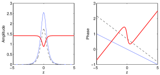
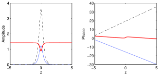
Figure 1: (color online). Amplitude and phase of two simultons (7) at $t=0$ with $V_{1}=2$, $V_{2}=1$, $a=1$, $k=0.5$, $q=0.5$; in the upper figures $p=1$, in the lower figures $p=-1$. Thin solid curve $E_{1}$, dashed curve $E_{2}$, thick solid curve $E_{3}$.

A simple analysis of (8) shows that, for any value of the parameters, the pulse amplitudes $U_{1}(\xi)$, $U_{2}(\xi)$ and $U_{3}(\xi)$ are even functions of $\xi$ and the phase constants satisfy $\phi_{1}+\phi_{2}+\phi_{3}=0$. On the other hand, if $k=0$ the phase profiles are all piecewise linear in $\xi$ and obey the condition $f_{1}(\xi)+f_{2}(\xi)+f_{3}(\xi)=0$ for $p\xi>0$ and $f_{1}(\xi)+f_{2}(\xi)+f_{3}(\xi)=\pi$ for $p\xi<0$. Whereas for $k\neq 0$ the phase profile $f_{3}(\xi)$ is nonlinear and $\cos[f_{1}(\xi)+f_{2}(\xi)+f_{3}(\xi)]$ is an odd function of $\xi$; moreover the kink pulse $E_{3}$ is “grey” if $k\neq 0$ and is “dark” if $k=0$. Such amplitude and phase front profiles prevent a net energy exchange among the three waves. It is important to point out that the condition $-1<Q<1$ leads to a speed $V$ that lies in-between the characteristic velocities $V_{1}$ and $V_{2}$ of the two bright pulses, i.e. $V_{1}>V>V_{2}$. The above described properties mean that TWRIS represent a significant generalization with respect to previously known three-wave solitons which exhibit a simple (constant) phase profile and correspond to the special case $k=q=0\,,\,r>0$ nozaki74 . In Fig.1 we plotted two characteristic examples of TWRIS amplitude and phase-fronts (7).

It is interesting to consider the physical meaning of the various TWRIS parameters appearing in (7). For a given choice of the characteristic linear velocities $V_{1}$ and $V_{2}$, we are left with the four independent parameters $p,k,q$, and $a$. We may note that $p$ is basically associated with the scaling of the wave amplitudes, as well as of the coordinates $z$ and $t$. The parameter $a$ determines the amplitude of the asymptotic plateau of the kink $E_{3}$. The value of $k$ provides the wave–number of a “carrier–wave”. The parameter $q$ adds a phase contribution which is linear in $z$ and $t$. Since the system (Stable Control of Pulse Speed in Parametric Three-Wave Solitons) is invariant under a transformation (2), without loss of generality we may set $a=1$, which reduces the number of essential parameters to just three, corresponding to the three symmetries of Eqs.(Stable Control of Pulse Speed in Parametric Three-Wave Solitons). The parameters $p,k,q$ in (7) may be more conveniently mapped into the parameters $V,\phi_{1},\phi_{2}$ of Eq.(8), which provide a more direct physical insight into the features of a TWRIS. Such a mapping is obtained by comparing Eqs.(7) with (8), and reads as: $V=2V_{1}V_{2}/[\,V_{1}+V_{2}-Q(V_{1}-V_{2})\,],\,\,\phi_{1}=qV_{2}(V_{1}-V)+\chi V+\omega,\,\,\phi_{2}=qV_{1}(V-V_{2})-\chi V-\omega$. The TWRIS is thus simply expressed in terms of its velocity $V$ and the two phase constants $\phi_{1}$ and $\phi_{2}$.

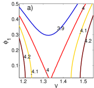
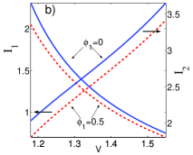
Figure 2: (color online). (a) phase constant $\phi_{1}$ versus velocity $V$ for different energies $I_{12}.$ (b) energies $I_{1}$, $I_{2}$ versus velocity $V$ for representative values of the phase constant $\phi_{1}$. In all cases $\phi_{2}=-\phi_{1}$, $V_{1}=2$, $V_{2}=1$.

Let us investigate what are the TWRIS properties for a fixed choice of the linear velocities $V_{1}$ and $V_{2}$, upon variations of its energy flows and transverse momentum. As an example, Fig. 2(a) shows the dependence of the phase constant $\phi_{1}$ on the locked velocity $V$, for the case where $\phi_{2}=-\phi_{1}$, with different values of the conserved energy $I_{12}$. Moreover, Fig. 2(b) illustrates the dependence of the energies $I_{1}$ and $I_{2}$ (which happen to be time–independent for a TWRIS) on the locked velocity $V$, for different choices of the phase constant $\phi_{1}=-\phi_{2}$. As it can be seen, the intensity and phase profiles, as well as the energy distribution among the different wave packets, strongly depend upon the value of the locked velocity $V$.

The next crucial issue is the propagation stability of TWRIS. A first insight into this problem may be provided by performing a linear stability analysis (LSA) as in Ref.conforti05 . Let us consider a perturbed TWRIS of the form

$$\tilde{E}_{n}(\xi,\tau)=(x_{n}(\xi)+P_{n}(\xi,\tau))e^{i\phi_{n}\tau},\quad n=1,2,3$$

where $x_{n}(\xi)=U_{n}(\xi)\exp[{if_{n}(\xi)}]$ is the soliton profile, and we consider a weak perturbation $|P_{n}|<<|x_{n}|$. By inserting the above ansatz in Eqs.(Stable Control of Pulse Speed in Parametric Three-Wave Solitons), and by retaining only linear terms in $P_{n}$, one obtains a linear system of PDEs. For the numerical analysis, these PDEs can be reduced to a system of ordinary differential equations $\dot{P}(\tau)=MP(\tau)$, by approximating the spatial derivatives with finite differences, where $P$ is the perturbation vector sampled on a finite grid. A necessary condition for the instability of a stationary solution $x_{n}(\xi)$ is that the matrix $M$ has at least one eigenvalue with positive real part. Numerical computations over a wide parameter range show that eigenvalues of $M$ exist with a positive real part whenever $p<0$. On the other hand, for $p>0$ the largest real part of the eigenvalues is equal to zero, which means that the TWRIS are only neutrally stable. Note that the instability condition $p<0$ leads to the inequality $V<V_{cr}=2V_{1}V_{2}/(V_{1}+V_{2})$. Extensive numerical integrations of Eqs.(Stable Control of Pulse Speed in Parametric Three-Wave Solitons) confirm that TWRIS with $V<V_{cr}$ ($V>V_{cr}$) are always unstable (stable). The propagation of either stable or unstable TWRIS is illustrated in Fig. 3, which shows the general feature of unstable solitons with $V<V_{cr}$. Namely, the simulton decays into a stable soliton with $V>V_{cr}$, and it emits a pulse in the wave $E_{3}$. It is quite remarkable that the dynamics of the decay from unstable into stable solitons may be exactly described by analytical solutions with variable velocity or boomerons calogero05 . A complete description of the parametric boomerons will be the subject of a more extended report.

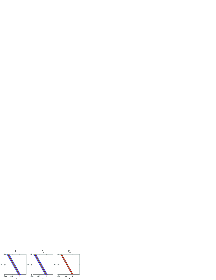
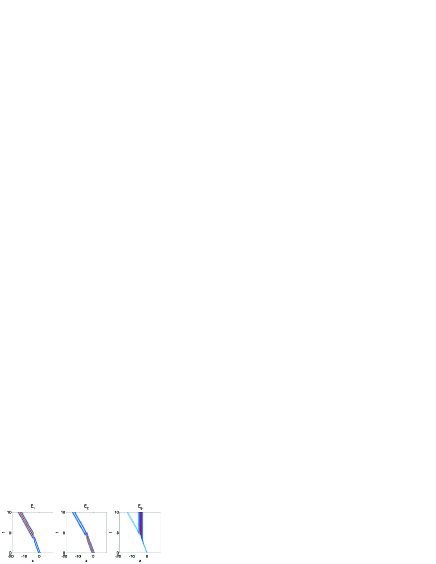
Figure 3: (color online). Propagation of stable and unstable simultons. The common parameters are $V_{1}=2$, $V_{2}=1$, $a=1$, $k=0.5$, $q=1$. For the stable simulton (upper figures) $p=1$ ($V=1.68>V_{cr}$, $\phi_{1}=0.5$, $\phi_{2}=2.2$), whereas for the unstable simulton (lower figures) $p=-1$ ($V=1.1<V_{cr}$, $\phi_{1}=1.43$, $\phi_{2}=-0.33$).

We performed further investigations of TWRIS stability by carrying out a multi-scale asymptotic analysis (MAA) pelinovsky95 ; buryak96 . The MAA aims to find the rate of growth $\lambda$ (with $\lambda<<1$) of small perturbations, by linearizing Eqs.(Stable Control of Pulse Speed in Parametric Three-Wave Solitons) around the soliton solution. This procedure leads to a linear eigenvalue problem, whose solution can be expressed as an asymptotic series in $\lambda$ mihalache97 . In this way, one obtains the following condition which defines the borderline between stable and unstable TWRIS

$$G=\frac{\partial(I_{12},\overline{I}_{23},\overline{J})}{\partial(\phi_{1},\phi_{2},V)}=0,$$ (9)

where $G$ is the Jacobian of the constants of motion $I_{12},\overline{I}_{23},\overline{J}$ with respect to $\phi_{1},\phi_{2},V$. Note that in (9) $\overline{I}_{23}$ and $\overline{J}$ are obtained by re–normalizing the divergent integrals (5) and (6) according to the prescription

$$\overline{I}_{23}=\frac{1}{2}\int_{-\infty}^{+\infty}(|E_{2}|^{2}+|E_{3}|^{2}-|E_{30}|^{2})dz,$$ (10)

$$\begin{split}\overline{J}=J-\frac{1}{4i}\int_{-\infty}^{+\infty}\big{[}(&E_{3}^{*}E_{3z}-E_{3}E_{3z}^{*})\bigg{[}\frac{|E_{30}|^{2}}{|E_{3}|^{2}}\bigg{]}\big{]}dz,\end{split}$$ (11)

where $|E_{30}|=\lim_{z\rightarrow\infty}|E_{3}|$ is the asymptotic amplitude of the kink kivshar95bis . Note that the availability of exact soliton solutions allows for the analytical calculation of the above integrals, hence of the condition (9), which is an extension of the well-known Vakhitov-Kolokov criterion. Thus (9) provides a sufficient stability condition, which can only be applied under specific constraints such as $\phi_{1}=\phi_{2}$. Indeed, in this case we find that the condition $G=0$ leads again to the previously found marginal stability condition $V=V_{cr}=2V_{1}V_{2}/(V_{1}+V_{2})$.

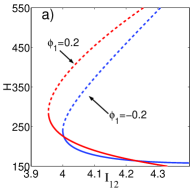
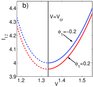
Figure 4: (color online). (a) Hamiltonian $H$ versus energy $I_{12}$ and (b) $I_{12}$ versus velocity $V$. Characteristic velocities are $V_{1}=2,V_{2}=1$ and $\phi_{2}=-0.2$. Dashed (solid) curves, unstable (stable) solitons.

A direct insight into the global stability properties of TWRIS for all possible values of their parameters can be obtained by means of a geometrical approach torner98 . Indeed, TWRIS may be obtained as solutions of the variational problem

$$\delta(H+\phi_{1}I_{12}-(\phi_{1}+\phi_{2})\overline{I}_{23}-V\overline{J})=0,$$ (12)

where $\delta$ is the Frechét derivative. In other words, TWRIS represent the extrema of the Hamiltonian (3), for a fixed value of the energies and momentum ($V,\phi_{1},\phi_{2}$ represent Lagrange multipliers). Stable triplets are obtained whenever such extrema coincide with a global minimum of $H$. Clearly, if multiple solutions exist with the same $I_{12},\overline{I}_{23},\overline{J}$, the stable solution is obtained on the lower branch of $H$. In this framework the condition (9) corresponds to solitons such that the normal vector to the three–dimensional surface $H=H(I_{12},\overline{I}_{23},\overline{J})$ lies in the space $H=const.$. The above geometrical considerations permit the visualization of the stability boundaries when considering a projection of the hyper-surface $H=H(I_{12},\overline{I}_{23},\overline{J})$ on the plane $(I_{12},H)$. For example, Fig. 4 displays the dependence of $H$ upon $I_{12}$ for the case $\phi_{1}=-\phi_{2}$, where the criterion (9) cannot be applied, and in the case $\phi_{1}=\phi_{2}$. Here it is evident that the two branches of the Hamiltonian merge exactly at $V=V_{cr}$: at this point, the normal to the $H$ curve is also orthogonal to the vertical axis. Interestingly enough, Fig. 4 shows that the borderline TWRIS corresponds to a minimum of the bright pulses energy $I_{12}$ with respect to $V$. To summarize, we have shown that different numerical and analytical methods concur in predicting that the TWRIS stability is determined by the condition $V>V_{cr}$.

Let us briefly discuss the experimental conditions for the observation of TWRIS in nonlinear optics. For instance, when considering a three-wave oeo interaction in a 5 cm-long bulk PPLN sample with $18\mu m$ periodicity, the field envelope carriers $\lambda_{E1}=1.5\mu m$, $\lambda_{E2}=0.8\mu m$, $\lambda_{E3}=1.8\mu m$, pulse durations of about $1ps$, TWRIS can be observed with field intensities of a few $MW/cm^{2}$.

In conclusion, we have described a novel three-parameter family of (1+1) bright-bright-dark soliton waves as exact solutions of the three-wave resonant interaction equation. These TWRI solitons exhibit nonlinear phase-fronts curvatures, and exist for a given range of their locked velocity and energy flows. Their propagation stability has been investigated with the upshot that stable triplets occur whenever their velocity $V$ is greater than a certain critical value $V_{cr}$. On the other hand, unstable solitons dynamically reshape into stable solitons with higher velocity. The remarkable properties of these parametric solitons may open the way to new possibilities for the control of coherent energy transport in various physical settings.

References

- (1) J. A. Armstrong, S. S. Jha, and N. S. Shiren, IEEE J. Quantum Electron. QE-6, 123 (1970).
- (2) V. E. Zakharov and S. V. Manakov, Sov. Phys. JETP Lett. 18, 243 (1973).
- (3) D. J. Kaup, Stud. Appl. Math. 55, 9 (1976).
- (4) A. Degasperis and S. Lombardo, Physica D 214, 157 (2006).
- (5) K. Nozaki and T. Taniuti, J. Phys. Soc. Jpn. 34, 796 (1973); Y. Ohsawa and K. Nozaki, J. Phys. Soc. Jpn. 36, 591 (1974).
- (6) E. Ibragimov and A. Struthers, Opt. Lett. 21, 1582 (1996).
- (7) A. V. Buryak et. al, Phys. Rep. 370, 63 (2002).
- (8) F. Calogero and A. Degasperis, Physica D 200, 242 (2005).
- (9) M. Conforti et. al, J. Opt. Soc. Am. B 22, 2178 (2005).
- (10) D. E. Pelinovsky, A. V. Buryak, and Y. S. Kivshar, Phys. Rev. Lett. 75, 591 (1995).
- (11) A. V. Buryak, Y. S. Kivshar, and S. Trillo, Phys. Rev. Lett. 77, 5210 (1996).
- (12) D. Mihalache et. al, Phys. Rev. E 56, R6294 (1997).
- (13) Y. S. Kivshar and W. Królikovski, Opt. Lett. 20, 1527 (1995).
- (14) L. Torner et. al, J. Opt. Soc. Am. B 15, 1476 (1998).