Use of specific Green’s functions for solving direct problems involving a heterogeneous rigid frame porous medium slab solicited by acoustic waves

Abstract

A domain integral method employing a specific Green’s function (i.e., incorporating some features of the global problem of wave propagation in an inhomogeneous medium) is developed for solving direct and inverse scattering problems relative to slab-like macroscopically inhomogeneous porous obstacles. It is shown how to numerically solve such problems, involving both spatially-varying density and compressibility, by means of an iterative scheme initialized with a Born approximation. A numerical solution is obtained for a canonical problem involving a two-layer slab.

1 Introduction

This work was initially motivated by two problems: i) the design problem connected with the determination of the optimal profile of a continuous and/or discontinuous spatial distribution of the material/geometric properties of porous materials for the absorption of sound [7] and ii) the retrieval of the spatially-varying mechanical and geometrical parameters of bone for the diagnosis of diseases such as osteoporosis [10].

Such inverse problems [20] can be decomposed into two sub-problems: i) the determination of the constitutive and conservation relations linking the various spatially-variable mechanical parameters of the porous medium to its response to an acoustic solicitation, and ii) the resolution of the wave equation in an inhomogeneous porous medium (for instance, within the Biot, or rigid frame approximations). Here we focus on the second point.

In [17], it is shown that the wave equation describing the propagation in a macroscopically-inhomogeneous porous medium in the rigid frame approximation can formally take the form of the usual acoustic wave equation in a macroscopically-inhomogeneous fluid (in which the microscopic features of the porous medium are homogenized) with spatial (and frequency) dependent compressibility $\kappa_{e}(\mathbf{x},\omega)$ and density $\rho_{e}(\mathbf{x},\omega)$.

The present work deals with a method of resolution of direct problems involving acoustic wave propagation in a macroscopically-inhomogeneous fluid medium, whose density and compressibility are both space dependent, this being a prerequisite to the resolution of related inverse problems.

This topic is also of great interest in quantum physics (inverse potential scattering [2, 37, 38, 39]), ocean acoustics [9, 8, 32, 11, 36, 12] (detection of inhomogeneities, sediment exploration, influence of seawater and seafloor composition and heterogenity on the long-range propagation of acoustic waves in the sea, …), seismology [1, 40, 42] (determination of the internal structure and composition of the Earth via seismic waves,…), geophysics [42, 25, 48, 44] (characterization of soil, detection of geological features such as hydrocarbon reservoirs, …), optics and electromagnetism [47, 41] (design and characterization of materials having specified response to waves, detection of flaws,…).

The wave equation in an inhomogeneous medium can be solved in a variety of manners: via the wave splitting method [33, 17, 30], the transfer matrix method [28, 4] (for piecewise constant media), integral methods [20, 39, 37], or purely numerical (e.g., finite-element [19] or finite-difference [5]) methods. The methods dedicated to inverse problems are wave splitting and linearisation [38, 39] techniques deriving from the integral formalism. The two most widely-known approximations for the Fredholm equations of the second kind involved in the integral formalism (at least when the density is constant in the acoustic context) are the Born approximation [35, 39] and the Rytov approximation [23]. We will focus on the Born approximation, despite the fact that several authors [27, 13] have shown that the Rytov approximation is valid under a less restrictive set of conditions than the Born approximation.

We postulate, and show, that the accuracy of the Born approximation can be increased by the use of the integral formulation together with a specific Green’s function [37, 39, 46]. In most of the articles dealing with the Born approximation and other linearisation methods, the problems are often simplified by considering the density to be constant. Herein, we consider both the compressibility and the density to be spatially-variable. This induces supplementary difficulties, because it can lead to meaningless integrals (involving first and/or second space derivatives of the density), especially when the variation of the density is not continuous, and/or because it requires the evaluation of the first space derivative of the pressure field. We will show how to deal with these problems.

The usual first-order Born approximation is an outcome of the integral formulation employing the free-space Green’s function (FSGF) and consists in approximating the pressure field in the integrand (corresponding to the pressure field inside the heterogeneity) by the field in the absence of the heterogeneity (i.e. the incident field), this being equivalent to the asssumption that the diffracted field is negligible compared to the incident field. Although this method usually provides good results for small contrasts between the mechanical parameters of the inhomogeneity and those of the host medium, its accuracy decreases in the case of dissipative media and larger contrasts.

Moreover, iterative schemes initialized with the zeroth-order Born or Rytov approximations often diverge in practice. This difficulty can be partially resolved by employing the modified or distorted Born approximation [39] which basically consist in acting on one of the three terms involved in the integrand (the Green’s function, the contrast function and the field inside the heterogeneity).

The method described herafter allows us to act on all three terms. The central idea of our method consists in reducing the eigenvalues of the kernel of the integrand (thought to be the cause of the difficulties with the usual iterative Born scheme) by employing a Green’s function–the so-called Specific Green’s function (SGF)– of a canonical problem which is close, in some sense, to the original problem. The specification of the initial solution was already treated in [46] in connection with the resolution of an inverse problem. The chosen problem (also canonical) is that of the diffraction of an incident plane wave, propagating in the host medium, by a two-component slab (each component being a homogeneous layer) considered as a single inhomogeneous slab. In the present instance, the close canonical problem involves a slab filled with a macroscopically-homogeneous fluid-saturated porous medium surrounded by the same fluid (air) medium as the original macroscopically-inhomogeneous fluid-saturated porous medium.

We will show, for this example: i) how to construct an appropriate specific Green’s function (SGF), ii) how to incorporate the latter into the integral formulation, and iii) how the resulting integral equation can be solved by an iterative scheme initialized by a modified Born approximation.

The results are compared to those of the analytic solutions (obtained by the transfer matrix method (TMM)) for the two-component slab and found to be in good agreement with the latter, both in transmission and reflection and for several angles of incidence. The iterative scheme initialized with the modified Born approximation converges rather rapidly, i.e., within $5$ to $7$ iterations for our example. This demonstrates the efficiency of our SGF interative scheme for the resolution of the direct problem relative to wave propagation in the presence of a macroscopically-inhomogeneous fluid-saturated porous slab.

2 Use of the specific Green’s functions in the domain integral formulation to solve direct scattering problems

2.1 An example of a direct scattering problem

The type of direct problem we deal with is illustrated in figure 1a. This problem involves spatially- dependent compressibility and density. As will be shown further on, the spatial variability, and discontinuity, of both these quantities, and in particular of the latter, can produce some difficulties in the domain integral formulations (but not in the TMM formulation). The wave equation for such problems is given in appendix A; to solve them in optimal manner, we treat the auxiliary problem depicted in figure 1b.

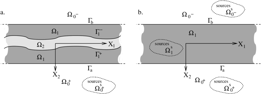
Figure 1: Configuration of the direct problem of a.: a fluid heterogeneity within a fluid-like slab, b.: diffraction of a wave radiated by applied sources from a fluid slab of boundaries $\Gamma_{a}$ and $\Gamma_{b}$ immersed in a fluid.

2.2 Specific Green’s function corresponding to the propagation of waves radiated by interior and exterior line sources in the presenece of a homogeneous fluid-like layer immersed in a homogeneous fluid host medium

2.2.1 Features of the problem

The sagittal plane (cross-section) view of the scattering configuration is given in figure 1b. As we are dealing with a Green’s function, the supports of the sources reduce to dots in the figure, i.e., the sources are line sources. The homogeneous fluid-like layer is oriented horizontally (i.e. the normal to both of its faces is along the $x_{2}$ axis); its thickness is $l$, and the medium $M^{1}$ therein is homogeneous. The geometry and composition of the layer are thus invariant with respect to $x_{3}$. $\Omega_{1}$ designates the trace of the layer in the $x_{1}-x_{2}$ cross-section plane. $\Gamma_{a}$ and $\Gamma_{b}$ designate the traces of the lower and upper faces respectively of the layer in the $x_{1}-x_{2}$ cross-section plane. The unit vectors normal to $\Gamma_{a}$ and $\Gamma_{b}$ are designated indistinctly by $\boldsymbol{\nu}$. The $x_{2}$ coordinates of $\Gamma_{a}$ and $\Gamma_{b}$ are designated by $a$ and $b$ respectively.

The layer is immersed in a (host) fluid $M^{0}$. The trace of the host medium domain below (above) the layer in the $x_{1}-x_{2}$ cross-section plane is designated by $\Omega_{0^{+}}$ ($\Omega_{0^{-}}$).

The (direct scattering) problem is to determine the response $g^{0^{+}}$ within $\Omega_{0^{+}}$, $g^{0^{-}}$ within $\Omega_{0^{-}}$ and $g^{1}$ within $\Omega_{1}$ for line sources that are located either within $\Omega_{0^{+}}$, $\Omega_{0^{-}}$ or $\Omega_{1}$. This response constitutes the specific Green’s function we are looking for.

Let $\mathbf{y}$ designate the vector from $O$ to the location of the line source. The Green’s function in $\Omega_{j}$ is designated by $g^{j}(\mathbf{x},\mathbf{y})$, which means the response at $\mathbf{x}$ due to line sources located at $\mathbf{y}$.

2.2.2 Governing equations

Rather than to solve directly for $g^{j}(\mathbf{x},\mathbf{y},t)$, we prefer to deal with its Fourier transform $g^{j}(\mathbf{x},\mathbf{y},\omega)$ defined by:

$$g^{j}(\mathbf{x},\mathbf{y},t)=\int_{-\infty}^{\infty}g^{j}(\mathbf{x},\mathbf{y},\omega)e^{-\mbox{i}\omega t}d\omega\mbox{; }j=0^{+},1,0^{-}$$ (1)

The mathematical translation of the boundary-value problem in the space-frequency domain is:

$$\left[\triangle+\left(k^{j}\right)^{2}\right]g^{j}\left(\mathbf{x},\mathbf{y},\omega\right)=-\delta(\mathbf{x}-\mathbf{y})\mbox{ : }\forall\mathbf{x}\in\Omega_{j}\mbox{, }j=0^{+},1,0^{-}\mbox{, }\mathbf{y}\in\Omega_{0^{+}}\mbox{, }\Omega_{1}\mbox{ or }\Omega_{0^{-}},$$ (2)

$$\begin{array}[]{ll}\displaystyle\forall\mathbf{x}\in\Gamma_{a}&\displaystyle\left\{\begin{array}[]{l}\displaystyle g^{0^{+}}\left(\mathbf{x},\mathbf{y},\omega\right)-g^{1}\left(\mathbf{x},\mathbf{y},\omega\right)=0\\[8.0pt] \displaystyle\frac{1}{\rho^{0}}\boldsymbol{\nu}(\mathbf{x})\cdot\nabla g^{0^{+}}\left(\mathbf{x},\mathbf{y},\omega\right)-\frac{1}{\rho^{1}}\boldsymbol{\nu}(\mathbf{x})\cdot\nabla g^{1}\left(\mathbf{x},\mathbf{y},\omega\right)=0\end{array}\right.\end{array}$$ (3)

$$\begin{array}[]{ll}\displaystyle\forall\mathbf{x}\in\Gamma_{b}&\displaystyle\left\{\begin{array}[]{l}\displaystyle g^{1}\left(\mathbf{x},\mathbf{y},\omega\right)-g^{0^{-}}\left(\mathbf{x},\mathbf{y},\omega\right)=0\\[8.0pt] \displaystyle\frac{1}{\rho^{1}}\boldsymbol{\nu}(\mathbf{x})\cdot\nabla g^{1}\left(\mathbf{x},\mathbf{y},\omega\right)-\frac{1}{\rho^{0}}\boldsymbol{\nu}(\mathbf{x})\cdot\nabla g^{0^{-}}\left(\mathbf{x},\mathbf{y},\omega\right)=0\end{array}\right.\end{array}$$ (4)

$$g^{j}\left(\mathbf{x},\mathbf{y},\omega\right)-G^{j}\left(\mathbf{x},\mathbf{y},\omega\right)\sim\mbox{ outgoing waves, }\mbox{ ; }\forall\mathbf{x}\in\Omega_{j}\mbox{ ; }j=0^{+},1,0^{-}\mbox{, }\|\mathbf{x}\|\rightarrow\infty$$ (5)

wherein $G^{j}$ is the free-space Green’s function in the medium $M^{j}$ given by

$$G^{j}(\mathbf{x},\mathbf{y},\omega)=\frac{i}{4}H_{0}^{(1)}(k^{j}(\|\mathbf{x}-\mathbf{y}\|)=\frac{\mbox{i}}{4\pi}\int_{-\infty}^{\infty}\exp\left(\mbox{i}k_{1}\left(x_{1}-y_{1}\right)+\mbox{i}k_{2}^{j}\left|x_{2}-y_{2}\right|\right)\frac{dk_{1}}{k_{2}^{j}}~{},$$ (6)

with $H_{0}^{(1)}$ the zeroth-order Hankel function of the first kind, $k_{2}^{j}=\sqrt{\left(k^{j}\right)^{2}-(k_{1})^{2}}$ such that $\Re\left(k_{2}^{j}\right)\geq 0$ and $\Im\left(k_{2}^{j}\right)\geq 0$, $j=0,1$ for $\omega\geq 0$.

2.2.3 Field representations

We shall henceforth: i) drop the $\omega$-dependence with the understanding that it is implicit in all the field functions and ii) employ the cartesian coordinates $(x_{1},x_{2})$ of $\mathbf{x}$ and $(y_{1},y_{2})$ of $\mathbf{y}$.

We use the separation of variables technique to obtain

$$g^{0^{+}}(\mathbf{x},\mathbf{y})=\mbox{H}_{\Omega_{0^{+}}}(\mathbf{y})G^{0^{+}}(\mathbf{x},\mathbf{y})+\int_{-\infty}^{\infty}B^{0^{+}}\exp\left(\mbox{i}k_{1}x_{1}+\mbox{i}k_{2}^{0}\left(x_{2}-a\right)\right)\frac{dk_{1}}{k_{2}^{0}}$$ (7)

$$g^{1}(\mathbf{x},\mathbf{y})=\mbox{H}_{\Omega_{1}}(\mathbf{y})G^{1}(\mathbf{x},\mathbf{y})+\int_{-\infty}^{\infty}\left(A^{1}\exp\left(-\mbox{i}k_{2}^{1}x_{2}\right)+B^{1}\exp\left(\mbox{i}k_{2}^{1}x_{2}\right)\right)\exp\left(\mbox{i}k_{1}x_{1}\right)\frac{dk_{1}}{k_{2}^{1}}$$ (8)

$$g^{0^{-}}(\mathbf{x},\mathbf{y})=\mbox{H}_{\Omega_{0^{-}}}(\mathbf{y})G^{0^{-}}(\mathbf{x},\mathbf{y})+\int_{-\infty}^{\infty}A^{0^{-}}\exp\left(\mbox{i}k_{1}x_{1}-\mbox{i}k_{2}^{0}\left(x_{2}-b\right)\right)\frac{dk_{1}}{k_{2}^{0}}$$ (9)

wherein $\mbox{H}_{\Omega_{j}}$ is the Heaviside function

$$\mbox{H}_{\Omega_{j}}(\mathbf{y})=\left\{\begin{array}[]{ll}\displaystyle 1&\displaystyle\mbox{if }\mathbf{y}\in\Omega_{j}\\[8.0pt] \displaystyle 0&\displaystyle\mbox{if }\mathbf{y}\in\Omega_{i}\mbox{, }i\neq j\end{array}\right.$$ (10)

2.2.4 Application of the transmission conditions

In cartesian coordinates and on account of the orientation of the two faces of the layer:

$$\boldsymbol{\nu}(\mathbf{x})\cdot\nabla\mathcal{F}=\frac{\partial}{\partial x_{2}}\mathcal{F}~{}.$$ (11)

After introducing the fields expressions, eqs.(7), (8) and (9) into the boundary conditions eqs.(3) and (4), we multiply these relations by $\exp\left(-\mbox{i}K_{1}x_{1}\right)$ and then integrate from $-\infty$ to $+\infty$, using the identity

$$\int_{-\infty}^{\infty}\exp\left(\mbox{i}\left(k_{1}-K_{1}\right)x_{1}\right)dx_{1}=2\pi\delta\left(k_{1}-K_{1}\right)\mbox{, $\delta\left(k_{1}-K_{1}\right)$ being the Kronecker symbol}$$ (12)

so as to obtain the matrix equation

$$\left(\!\begin{array}[]{llll}\displaystyle 1&\displaystyle\frac{-k_{2}^{0}e^{-\mbox{i}k_{2}^{1}a}}{k_{2}^{1}}&\displaystyle\frac{-k_{2}^{0}e^{\mbox{i}k_{2}^{1}a}}{k_{2}^{1}}&\displaystyle 0\\[8.0pt] \displaystyle 1&\displaystyle\frac{\rho^{0}e^{-\mbox{i}k_{2}^{1}a}}{\rho^{1}}&\displaystyle\frac{-\rho^{0}e^{\mbox{i}k_{2}^{1}a}}{\rho^{1}}&\displaystyle 0\\[8.0pt] \displaystyle 0&\displaystyle\frac{-k_{2}^{0}e^{-\mbox{i}k_{2}^{1}b}}{k_{2}^{1}}&\displaystyle\frac{-k_{2}^{0}e^{\mbox{i}k_{2}^{1}b}}{k_{2}^{1}}&\displaystyle 1\\[8.0pt] \displaystyle 0&\displaystyle\frac{-\rho^{0}e^{-\mbox{i}k_{2}^{1}b}}{\rho^{1}}&\displaystyle\frac{\rho^{0}e^{\mbox{i}k_{2}^{1}a}}{\rho^{1}}&\displaystyle 1\end{array}\!\right)\!\left(\!\begin{array}[]{l}\displaystyle B^{0^{+}}\\[8.0pt] \displaystyle A^{1}\\[8.0pt] \displaystyle B^{1}\\[8.0pt] \displaystyle A^{0^{-}}\\[8.0pt] \end{array}\!\right)=\frac{\mbox{i}e^{-\mbox{i}k_{1}y_{1}}}{4\pi}\left(\!\begin{array}[]{l}\displaystyle-e^{\mbox{i}k_{2}^{0}\left(y_{2}-a\right)}\mbox{H}_{\Omega_{0^{+}}}-\frac{k_{2}^{0}}{k_{2}^{1}}e^{\mbox{i}k_{2}^{1}\left(a-y_{2}\right)}\mbox{H}_{\Omega_{1}}\\[8.0pt] \displaystyle e^{\mbox{i}k_{2}^{0}\left(y_{2}-a\right)}\mbox{H}_{\Omega_{0^{+}}}-\frac{\rho^{0}}{\rho^{1}}e^{\mbox{i}k_{2}^{1}\left(a-y_{2}\right)}\mbox{H}_{\Omega_{1}}\\[8.0pt] \displaystyle-e^{\mbox{i}k_{2}^{0}\left(b-y_{2}\right)}\mbox{H}_{\Omega_{0^{-}}}+\frac{k_{2}^{0}}{k_{2}^{1}}e^{\mbox{i}k_{2}^{1}\left(y_{2}-b\right)}\mbox{H}_{\Omega_{1}}\\[8.0pt] \displaystyle e^{\mbox{i}k_{2}^{0}\left(b-y_{2}\right)}\mbox{H}_{\Omega_{0^{-}}}+\frac{\rho^{0}}{\rho^{1}}e^{\mbox{i}k_{2}^{1}\left(y_{2}-b\right)}\mbox{H}_{\Omega_{1}}\\[8.0pt] \end{array}\!\right)$$ (13)

2.2.5 Final expressions of the specific Green’s function

Once the matrix system (13) is solved for $B^{0^{+}}$, $A^{1}$, $B^{1}$ and $A^{0^{-}}$, and these expressions are introduced into the expressions of the fields (7), (8), (9), we get:

$$g^{0^{+}}(\mathbf{x},\mathbf{y})=\frac{\mbox{i}}{4\pi}\int_{-\infty}^{\infty}e^{[\mbox{i}k_{1}\left(x_{1}-y_{1}\right)+\mbox{i}k_{2}^{0}|x_{2}-y_{2}|]}\mbox{H}_{\Omega_{0^{+}}}\frac{dk_{1}}{k_{2}^{0}}+\\ \int_{-\infty}^{\infty}\frac{e^{[\mbox{i}k_{1}\left(x_{1}-y_{1}\right)+\mbox{i}k_{2}^{0}x_{2}]}}{4\pi\left(2\alpha^{0}\alpha^{1}\cos\left(k_{2}^{1}l\right)-\mbox{i}\left((\alpha^{0})^{2}+(\alpha^{1})^{2}\right)\sin\left(k_{2}^{1}l\right)\right)}\times\\ \left[e^{\mbox{i}k_{2}^{0}\left(y2-2a\right)}\sin\left(k_{2}^{1}l\right)\left((\alpha^{0})^{2}-(\alpha^{1})^{2}\right)\frac{\mbox{H}_{\Omega_{0^{+}}}}{k_{2}^{0}}+2\mbox{i}e^{-\mbox{i}k_{2}^{0}\left(y_{2}+l\right)}\alpha^{1}\alpha^{0}\frac{\mbox{H}_{\Omega_{0^{-}}}}{k_{2}^{0}}+\right.\\ \left.2\mbox{i}e^{-\mbox{i}k_{2}^{0}a}\alpha^{1}\left(\alpha^{1}\cos\left(k_{2}^{1}\left(y_{2}-b\right)\right)-\mbox{i}\alpha^{0}\sin\left(k_{2}^{1}\left(y_{2}-b\right)\right)\right)\frac{\mbox{H}_{\Omega_{1}}}{k_{2}^{1}}\right]dk_{1}~{},$$ (14)

$$g^{1}(\mathbf{x},\mathbf{y})=\frac{\mbox{i}}{4\pi}\int_{-\infty}^{\infty}e^{[\mbox{i}k_{1}\left(x_{1}-y_{1}\right)+\mbox{i}k_{2}^{1}|x_{2}-y_{2}|]}\mbox{H}_{\Omega_{1}}\frac{dk_{1}}{k_{2}^{1}}+\\ \int_{-\infty}^{\infty}\frac{\mbox{i}e^{\mbox{i}k_{1}\left(x_{1}-y_{1}\right)}}{4\pi\left(2\alpha^{0}\alpha^{1}\cos\left(k_{2}^{1}l\right)-\mbox{i}\left((\alpha^{0})^{2}+(\alpha^{1})^{2}\right)\sin\left(k_{2}^{1}l\right)\right)}\times\\ \left[2e^{\mbox{i}k_{2}^{0}\left(y_{2}-a\right)}\left(\alpha^{1}\alpha^{0}\cos\left(k_{2}^{1}\left(x_{2}-b\right)\right)-\mbox{i}\left(\alpha^{0}\right)^{2}\sin\left(k_{2}^{1}\left(x_{2}-b\right)\right)\right)\frac{\mbox{H}_{\Omega_{0^{+}}}}{k_{2}^{0}}+\right.\\ 2e^{\mbox{i}k_{2}^{0}\left(b-y_{2}\right)}\left(\alpha^{1}\alpha^{0}\cos\left(k_{2}^{1}\left(a-x_{2}\right)\right)-\mbox{i}\left(\alpha^{0}\right)^{2}\sin\left(k_{2}^{1}\left(a-x_{2}\right)\right)\right)\frac{\mbox{H}_{\Omega_{0^{-}}}}{k_{2}^{0}}+\\ \left.\left(\left((\alpha^{1})^{2}-(\alpha^{0})^{2}\right)\cos\left(k_{2}^{1}\left(x_{2}+y_{2}-a-b\right)\right)+\exp\left(\mbox{i}k_{2}^{1}l\right)\left(\alpha^{0}-\alpha^{1}\right)^{2}\cos\left(k_{2}^{1}\left(x_{2}-y_{2}\right)\right)\right)\frac{\mbox{H}_{\Omega_{1}}}{k_{2}^{1}}\right]dk_{1}~{},$$ (15)

$$g^{0^{-}}(\mathbf{x},\mathbf{y})=\frac{\mbox{i}}{4\pi}\int_{-\infty}^{\infty}e^{[\mbox{i}k_{1}\left(x_{1}-y_{1}\right)+\mbox{i}k_{2}^{0}|x_{2}-y_{2}|]}\mbox{H}_{\Omega_{0^{-}}}\frac{dk_{1}}{k_{2}^{0}}+\\ \int_{-\infty}^{\infty}\frac{e^{[\mbox{i}k_{1}\left(x_{1}-y_{1}\right)-\mbox{i}k_{2}^{0}x_{2}]}}{4\pi\left(2\alpha^{0}\alpha^{1}\cos\left(k_{2}^{1}l\right)-\mbox{i}\left((\alpha^{0})^{2}+(\alpha^{1})^{2}\right)\sin\left(k_{2}^{1}l\right)\right)}\times\\ \left[2\mbox{i}e^{-\mbox{i}k_{2}^{0}\left(l-y_{2}\right)}\alpha^{1}\alpha^{0}\frac{\mbox{H}_{\Omega_{0^{+}}}}{k_{2}^{0}}+e^{-\mbox{i}k_{2}^{0}\left(y2-2b\right)}\sin\left(k_{2}^{1}l\right)\left((\alpha^{0})^{2}-(\alpha^{1})^{2}\right)\frac{\mbox{H}_{\Omega_{0^{-}}}}{k_{2}^{0}}+\right.\\ \left.2\mbox{i}e^{\mbox{i}k_{2}^{0}b}\alpha^{1}\left(\alpha^{1}\cos\left(k_{2}^{1}\left(a-y_{2}\right)\right)-\mbox{i}\alpha^{0}\sin\left(k_{2}^{1}\left(a-y_{2}\right)\right)\right)\frac{\mbox{H}_{\Omega_{1}}}{k_{2}^{1}}\right]dk_{1}~{}.$$ (16)

2.3 Use of a specific Green’s function to solve the direct problem of pressure wave scattered by an inhomogeneous fluid-filled slab

We treat the 2D fluid acoustic direct problem illustrated in figure 2. In the absence of the heterogeneity, occupying the domain $\Omega_{2}$, the configuration is that of the closed layer domain $\Omega_{1}$ occupied by a known homogeneous fluid $M^{1}$ with (spatially-constant) acoustic parameters ($k^{1}$, $\rho^{1}$), surrounded by the open domain $\Omega_{0}$ occupied by a known homogeneous fluid $M^{0}$ with (spatially-constant) acoustic parameters ($k^{0}$, $\rho^{0}$).

In the presence of the heterogeneity, localized to the domain $\Omega_{2}\in\Omega_{1}$, the problem is to solve the scattering problem for spatially-varying acoustic parameter functions ($k^{2}(\mathbf{x})$, $\rho^{2}(\mathbf{x})$) of the medium $M^{2}$ filling $\Omega_{2}$ in the subdomains $\Omega_{0^{+}}$ and $\Omega_{0^{-}}$ when the slab is probed by an incident wave.

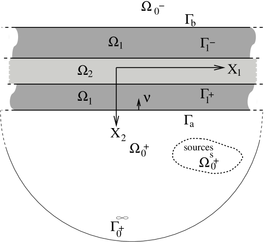
Figure 2: Configuration of the direct problem of a fluid heterogeneity within a fluid-like slab.

2.3.1 Governing equations for scattering from a heterogeneous layer, included between $\Gamma_{a}$ and $\Gamma_{b}$, probed by a cylindrical wave radiated by a cylindrical source whose support is $\Omega_{0^{+}}^{s}$

Let $\Omega_{1}=\widetilde{\Omega}_{1}\,\cup\,\Omega_{2}$. Then the governing equations for the pressure field are:

$$\left[\triangle+(k^{0})^{2}\right]p^{0^{+}}(\mathbf{x})=-s^{0}(\mathbf{x})\mbox{; }\mathbf{x}\in\Omega_{0^{+}},$$ (17)

$$\left[\triangle+\left(k(\mathbf{x})\right)^{2}\right]p^{1}(\mathbf{x})=\frac{\nabla\rho(\mathbf{x})}{\rho(\mathbf{x})}\cdot\nabla p^{1}(\mathbf{x})\mbox{; }\mathbf{x}\in\Omega_{1},$$ (18)

$$k(\mathbf{x})=\left\{\begin{array}[]{lll}\displaystyle k^{1}&\displaystyle;&\displaystyle\mathbf{x}\in\widetilde{\Omega}_{1}\\[8.0pt] \displaystyle k^{2}(\mathbf{x})&\displaystyle;&\displaystyle\mathbf{x}\in\Omega_{2}\end{array}\right.$$ (19)

$$\rho(\mathbf{x})=\left\{\begin{array}[]{lll}\displaystyle\rho^{1}&\displaystyle;&\displaystyle\mathbf{x}\in\widetilde{\Omega}_{1}\\[8.0pt] \displaystyle\rho^{2}(\mathbf{x})&\displaystyle;&\displaystyle\mathbf{x}\in\Omega_{2}\end{array}\right.$$ (20)

$$\left[\triangle+(k^{0})^{2}\right]p^{0^{-}}(\mathbf{x})=0\mbox{; }\mathbf{x}\in\Omega_{0^{-}},$$ (21)

$$p^{0+}(\mathbf{x})-p^{1}(\mathbf{x})=0\mbox{; }\mathbf{x}\in\Gamma_{a},$$ (22)

$$\frac{1}{\rho^{0}}\boldsymbol{\nu}(\mathbf{x})\cdot\nabla p^{0+}(\mathbf{x})-\frac{1}{\rho^{1}}\boldsymbol{\nu}(\mathbf{x})\cdot\nabla p^{1}(\mathbf{x})=0\mbox{; }\mathbf{x}\in\Gamma_{a},$$ (23)

$$p^{1}(\mathbf{x})-p^{0^{-}}(\mathbf{x})=0\mbox{; }\mathbf{x}\in\Gamma_{b},$$ (24)

$$\frac{1}{\rho^{1}}\boldsymbol{\nu}(\mathbf{x})\cdot\nabla p^{1}(\mathbf{x})-\frac{1}{\rho^{0}}\boldsymbol{\nu}(\mathbf{x})\cdot\nabla p^{0^{-}}(\mathbf{x})=0\mbox{; }\mathbf{x}\in\Gamma_{b},$$ (25)

$$p^{0^{+}}(\mathbf{x})\mbox{, }p^{1}(\mathbf{x})\mbox{ and }p^{0^{-}}(\mathbf{x})\sim\mbox{ outgoing waves, }\left\|\mathbf{x}\right\|\rightarrow\infty$$ (26)

The previously-given governing equations for the specific Green’s function can be rewritten as:

$$\left[\triangle+(K(\mathbf{x}))^{2}\right]g(\mathbf{x},\mathbf{y})=-\delta(\mathbf{x}-\mathbf{y})\mbox{; }\mathbf{x}\in\mathbb{R}^{2}\mbox{, }\mathbf{y}\in\mathbb{R}^{2}$$ (27)

$$K(\mathbf{x})=\left\{\begin{array}[]{lll}\displaystyle k^{0}&\displaystyle;&\displaystyle\mathbf{x}\in\Omega_{0^{+}}\,\cup\,\Omega_{0^{-}}\\[8.0pt] \displaystyle k^{1}&\displaystyle;&\displaystyle\mathbf{x}\in\Omega_{1}\end{array}\right.$$ (28)

$$g(\mathbf{x},\mathbf{y})=\left\{\begin{array}[]{lll}\displaystyle g^{0}(\mathbf{x},\mathbf{y})&\displaystyle;&\displaystyle\mathbf{x}\in\Omega_{0^{+}}\,\cup\,\Omega_{0^{-}}\\[8.0pt] \displaystyle g^{1}(\mathbf{x},\mathbf{y})&\displaystyle;&\displaystyle\mathbf{x}\in\Omega_{1}\end{array}\right.$$ (29)

$$g^{0+}(\mathbf{x},\mathbf{y})-g^{1}(\mathbf{x},\mathbf{y})=0\mbox{; }\mathbf{x}\in\Gamma_{a},$$ (30)

$$\frac{1}{\rho^{0}}\boldsymbol{\nu}(\mathbf{x})\cdot\nabla g^{0+}(\mathbf{x},\mathbf{y})-\frac{1}{\rho^{1}}\boldsymbol{\nu}(\mathbf{x})\cdot\nabla g^{1}(\mathbf{x},\mathbf{y})=0\mbox{; }\mathbf{x}\in\Gamma_{a},$$ (31)

$$g^{1}(\mathbf{x},\mathbf{y})-g^{0^{-}}(\mathbf{x},\mathbf{y})=0\mbox{; }\mathbf{x}\in\Gamma_{b},$$ (32)

$$\frac{1}{\rho^{1}}\boldsymbol{\nu}(\mathbf{x})\cdot\nabla g^{1}(\mathbf{x},\mathbf{y})-\frac{1}{\rho^{0}}\boldsymbol{\nu}(\mathbf{x})\cdot\nabla g^{0^{-}}(\mathbf{x},\mathbf{y})=0\mbox{; }\mathbf{x}\in\Gamma_{b},$$ (33)

$$g(\mathbf{x},\mathbf{y})\sim\mbox{ outgoing waves, }\left\|\mathbf{x}\right\|\rightarrow\infty$$ (34)

2.3.2 Towards a domain integral representation of the pressure field in $\Omega_{0^{+}}$

In obvious short-hand notation (in addition: $\partial_{\nu}:=\boldsymbol{\nu}\cdot\nabla$), we obtain from the previous governing equations:

$$g^{0^{+}}\left[\triangle+(k^{0})^{2}\right]p^{0^{+}}=-g^{0^{+}}s^{0}\mbox{ ; in }\Omega_{0^{+}}$$ (35)

$$p^{0^{+}}\left[\triangle+(k^{0})^{2}\right]g^{0^{+}}=-p^{0^{+}}\delta\mbox{ ; in }\Omega_{0^{+}}$$ (36)

so that integrating the difference of these two equations over $\Omega_{0^{+}}$, we obtain

$$\int_{\Omega_{0}}\left(g^{0^{+}}\triangle p^{0^{+}}-p^{0^{+}}\triangle g^{0^{+}}\right)d\Omega=-\int_{\Omega_{0}}g^{0^{+}}s^{0}d\Omega+\int_{\Omega_{0}}p^{0^{+}}\delta d\Omega$$ (37)

or, after use of Green’s theorem and the sifting property of the $\delta$ distribution:

$$\begin{array}[]{l}\displaystyle\int_{\Gamma_{0^{+}}^{\infty}}\left(g^{0^{+}}\partial_{\nu}p^{0^{+}}-p^{0^{+}}\partial_{\nu}g^{0^{+}}\right)d\gamma+\\[8.0pt] \displaystyle\int_{\Gamma_{a}}\left(g^{0^{+}}\partial_{\nu}p^{0^{+}}-p^{0^{+}}\partial_{\nu}g^{0^{+}}\right)d\gamma+\int_{\Omega_{0}}g^{0^{+}}s^{0}d\Omega=p^{0^{+}}(\mathbf{y})\mbox{H}_{\Omega^{0^{+}}}(\mathbf{y})\end{array}$$ (38)

We develop, for the domain integral representation of this pressure field, the integration over $\Gamma_{0^{+}}^{\infty}$, so that to obtain:

$$\int_{\Gamma_{0^{+}}^{\infty}}\left(g^{0^{+}}\partial_{\nu}p^{0^{+}}-p^{0^{+}}\partial_{\nu}g^{0^{+}}\right)d\gamma=\int_{\Gamma_{0^{+}}^{\infty}}g^{0^{+}}\left[\partial_{\nu}p^{0^{+}}-\mbox{i}k^{0}p^{0^{+}}\right]d\gamma-\int_{\Gamma_{0^{+}}^{\infty}}p^{0^{+}}\left[\partial_{\nu}g^{0^{+}}-\mbox{i}k^{0}g^{0^{+}}\right]d\gamma$$ (39)

It is readily shown that both of the integrals on the right hand side of this expression vanish due to the fact that both $p^{0^{+}}$ and $g^{0^{+}}$ satisfy the (frequency domain) rediation condition at infinity.

2.3.3 Towards a domain integral representation of the pressure field in $\Omega_{1}$

In obvious short-hand notation, we obtain from the previous governing equations:

$$\left[\triangle+(k(\mathbf{x}))^{2}\right]p^{1}=\frac{\nabla\rho}{\rho}\cdot\nabla p^{1}\mbox{ ; }\Rightarrow\left[\triangle+(k^{1})^{2}\right]p^{1}=\left[(k^{1})^{2}-(k(x))^{2}\right]p^{1}+\frac{\nabla\rho}{\rho}\cdot\nabla p^{1}=-\sigma(\mathbf{x})$$ (40)

Consequently,

$$g^{1}\left[\triangle+(k^{1})^{2}\right]p^{1}=-g^{1}\sigma\delta\mbox{ ; in }\Omega_{1}$$ (41)

$$p^{1}\left[\triangle+(k^{1})^{2}\right]g^{1}=-p^{1}\delta\mbox{ ; in }\Omega_{1}$$ (42)

so that, integrating the difference of these two equations over $\Omega_{1}$, and after use of Green’s theorem and the sifting property of the $\delta$ distribution, we obtain:

$$-\int_{\Gamma_{a}}\left(g^{1}\partial_{\nu}p^{1}-p^{1}\partial_{\nu}g^{1}\right)d\gamma+\int_{\Gamma_{b}}\left(g^{1}\partial_{\nu}p^{1}-p^{1}\partial_{\nu}g^{1}\right)d\gamma+\int_{\Omega_{1}}g^{1}\sigma d\Omega=p^{1}(\mathbf{y})\mbox{H}_{\Omega^{1}}(\mathbf{y})$$ (43)

which yields, on account of the transmission conditions:

$$-\int_{\Gamma_{a}}\left(g^{0^{+}}\partial_{\nu}p^{0^{+}}-p^{0^{+}}\partial_{\nu}g^{0^{+}}\right)d\gamma+\int_{\Gamma_{b}}\left(g^{0^{-}}\partial_{\nu}p^{0^{-}}-p^{0^{-}}\partial_{\nu}g^{0^{-}}\right)d\gamma+\frac{\rho^{0}}{\rho^{1}}\int_{\Omega_{1}}g^{1}\sigma d\Omega=\\ \frac{\rho^{0}}{\rho^{1}}p^{1}(\mathbf{y})\mbox{H}_{\Omega^{1}}(\mathbf{y})$$ (44)

2.3.4 Towards a domain integral representation of the pressure field in $\Omega_{0^{-}}$

In obvious short-hand notation, we obtain from the previous governing equations:

$$g^{0^{-}}\left[\triangle+(k^{0})^{2}\right]p^{0^{-}}=0\mbox{ ; in }\Omega_{0^{-}}~{},$$ (45)

$$p^{0^{-}}\left[\triangle+(k^{0})^{2}\right]g^{0^{-}}=-p^{0^{-}}\delta\mbox{ ; in }\Omega_{0^{-}}~{},$$ (46)

so that, integrating the difference of these two equations over $\Omega_{0^{-}}$, and following the procedure used in the last two subsections, we obtain:

$$-\int_{\Gamma_{b}}\left(g^{0^{-}}\partial_{\nu}p^{0^{-}}-p^{0^{-}}\partial_{\nu}g^{0^{-}}\right)d\gamma=p^{0^{-}}(\mathbf{y})\mbox{H}_{\Omega^{0^{-}}}(\mathbf{y})~{}.$$ (47)

2.3.5 Domain integral representations, without boundary terms, of the pressure fields in $\Omega_{0^{+}}$, $\Omega_{1}$ and $\Omega_{0^{-}}$

The addition of (38), (44) and (47) gives

$$\int_{\Omega_{0^{+}}}g^{0^{+}}s^{0}d\Omega+\frac{\rho^{0}}{\rho^{1}}\int_{\Omega_{1}}g^{1}\sigma d\Omega=p^{0^{+}}(\mathbf{y})\mbox{H}_{\Omega^{0^{+}}}(\mathbf{y})+p^{1}(\mathbf{y})\mbox{H}_{\Omega^{1}}(\mathbf{y})+p^{0^{+}}(\mathbf{y})\mbox{H}_{\Omega^{0^{+}}}(\mathbf{y})~{},$$ (48)

from which it ensues, on account of the properties of the domain Heaviside function:

$$p^{0^{+}}(\mathbf{y})=\int_{\Omega_{0^{+}}}g^{0^{+}}s^{0}d\Omega+\frac{\rho^{0}}{\rho^{1}}\int_{\Omega_{1}}g^{1}(\mathbf{x},\mathbf{y})\left[\left(k(\mathbf{x})^{2}-(k^{1})^{2}\right)-\frac{\nabla\rho}{\rho}\cdot\nabla\right]p^{1}(\mathbf{x})d\Omega\mbox{, }\forall\mathbf{y}\in\Omega_{0^{+}}~{},$$ (49)

$$p^{1}(\mathbf{y})=\frac{\rho^{1}}{\rho^{0}}\int_{\Omega_{0^{+}}}g^{0^{+}}s^{0}d\Omega+\int_{\Omega_{1}}g^{1}(\mathbf{x},\mathbf{y})\left[\left(k(\mathbf{x})^{2}-(k^{1})^{2}\right)-\frac{\nabla\rho}{\rho}\cdot\nabla\right]p^{1}(\mathbf{x})d\Omega\mbox{, }\forall\mathbf{y}\in\Omega_{1}~{},$$ (50)

$$p^{0^{-}}(\mathbf{y})=\int_{\Omega_{0^{+}}}g^{0^{+}}s^{0}d\Omega+\frac{\rho^{0}}{\rho^{1}}\int_{\Omega_{1}}g^{1}(\mathbf{x},\mathbf{y})\left[\left(k(\mathbf{x})^{2}-(k^{1})^{2}\right)-\frac{\nabla\rho}{\rho}\cdot\nabla\right]p^{1}(\mathbf{x})d\Omega\mbox{, }\forall\mathbf{y}\in\Omega_{0^{-}}~{}.$$ (51)

2.3.6 Other integral representations, without boundary terms, of the pressure fields in $\Omega_{0^{+}}$, $\Omega_{1}$ and $\Omega_{0^{-}}$

Let $g_{i}^{j}(\mathbf{x},\mathbf{y})$ correspond to $\mathbf{y}\in\Omega_{i}$ and $\mathbf{x}\in\Omega_{j}$. Reciprocity implies $\displaystyle g_{i}^{j}(\mathbf{x},\mathbf{y})=\frac{\rho^{j}}{\rho^{i}}g_{j}^{i}(\mathbf{y},\mathbf{x})$. The integral representations (49), (50) and (51) can finally be written in the condensed form (recalling that $\Omega=\Omega_{0^{+}}\cup\Omega_{1}\cup\Omega_{0^{-}}$):

$$p(\mathbf{y},\omega)=\int_{\Omega_{0^{+}}^{s}}g_{0^{+}}(\mathbf{y},\mathbf{x})s^{0}(\mathbf{x})d\Omega(\mathbf{x})+\int_{\Omega_{1}}g_{1}(\mathbf{y},\mathbf{x})\left[\left(k(\mathbf{x})^{2}-(k^{1})^{2}\right)-\frac{\nabla\rho}{\rho}\cdot\nabla\right]p(\mathbf{x})d\Omega(\mathbf{x})\mbox{; }\forall\mathbf{y}\in\Omega$$ (52)

3 Comments on the integral representation of the field

Eq. (52) can be written as:

$$p^{s}(\mathbf{y}):=p(\mathbf{y})-\int_{\Omega_{0^{+}}^{s}}g_{0^{+}}(\mathbf{y},\mathbf{x})s^{0}(\mathbf{x})d\Omega(\mathbf{x})=\\ \int_{\Omega_{1}}g_{1}(\mathbf{y},\mathbf{x})\left[\left(k(\mathbf{x})^{2}-(k^{1})^{2}\right)-\frac{\nabla\rho}{\rho}\cdot\nabla\right]p(\mathbf{x})d\Omega(\mathbf{x})\mbox{; }\forall\mathbf{y}\in\Omega~{},$$ (53)

wherein $p^{s}(\mathbf{y})$ is the field scattered by the inhomogeneity of the slab.

This can be compared to the more common formulation employing the free-space Green’s function ($G^{0}(\mathbf{x},\mathbf{y})$):

$$p^{d}(\mathbf{y}):=p(\mathbf{y},\omega)-\int_{\Omega_{0^{+}}^{s}}G^{0}(\mathbf{y},\mathbf{x})s^{0}(\mathbf{x})d\Omega(\mathbf{x})=\\ \int_{\Omega_{1}}G^{0}(\mathbf{y},\mathbf{x})\left[(k(\mathbf{x}))^{2}-(k^{0})^{2}-\frac{\nabla\rho}{\rho}\cdot\nabla\right]p(\mathbf{x})d\Omega(\mathbf{x})\mbox{; }\forall\mathbf{y}\in\Omega~{},$$ (54)

wherein $p^{d}(\mathbf{y},\omega)$ is the field diffracted by the entire inhomogeneous slab (including the slab itself and its inhomogeneities). The SGF formulation thus appears to be more suitable than the FSGF formulation, because the scattered field $p^{s}(\mathbf{y},\omega)$ accounts at the outset for more of the physics of the interaction of the obstacle with the incident wave than $p^{d}(\mathbf{y})$.

It can be shown that the neglected field is generally smaller in the SGF formulation than in the FSFG formulation. Effectively, when the SGF formulation is employed, the zeroth order Born approximation consists in neglecting $\displaystyle\int_{\Omega_{1}}g_{1}(\mathbf{y},\mathbf{x})\left[\left(k(\mathbf{x})^{2}-(k^{1})^{2}\right)-\frac{\nabla\rho}{\rho}\cdot\nabla\right]p(\mathbf{x})d\Omega(\mathbf{x})$ compared to $\displaystyle\int_{\Omega_{0^{+}}^{s}}g_{0^{+}}(\mathbf{y},\mathbf{x})s^{0}(\mathbf{x})d\Omega(\mathbf{x})$ whereas when the FSFG formulation is employed, the zeroth-order Born approximation consists in neglecting $\int_{\Omega_{1}}G^{0}(\mathbf{y},\mathbf{x})\left[(k(\mathbf{x}))^{2}-(k^{0})^{2}-\frac{\nabla\rho}{\rho}\cdot\nabla\right]p(\mathbf{x})d\Omega(\mathbf{x})$ in comparison to $\int_{\Omega_{0^{+}}^{s}}G^{0}(\mathbf{y},\mathbf{x})s^{0}(\mathbf{x})d\Omega(\mathbf{x})$.

The use of the SGF includes some multiple reflections, while the FSGF formulation combined with the Born approximation does not apply to high contrasts, because the employed linearization tacitly precludes multiple reflections.

Finally, when the density is constant, the contrast component of the kernels of both formulations reduce to

$$(k^{j})^{2}\left(\left(\frac{k(x_{2})}{k^{j}}\right)^{2}-1\right)=(k^{j})^{2}\left(\left(\frac{\frac{\omega}{c(x_{2})}+\mbox{i}\alpha(\omega,x_{2})}{k^{j}}\right)^{2}-1\right)$$ (55)

wherein $\alpha(\omega,x_{2})$ is the absorption coefficient and $j=0$ for the FSGF and $j=1$ for SGF. It has been shown in [26] that the Born approximation is reasonable if the phase shift introduced by the inhomogeneous medium is less than $\pi$, i.e., weak and smooth heterogeneities of simple shape. The shift depends not only on the size, but also on the kernel, (eq. 55), i.e., on the frequency, on the absorption, and on the contrast between the two phase velocities. The use of the SGF, when the initial configuration is a homogeneous slab filled with a fluid-saturated porous material, allows us: i) to reduce the frequency dependence of the kernel, ii) to reduce the kernel itself by taking into account a phase-velocity that is closer to that of the host medium and also by taking into account the absorption (dissipation) of the material, and iii) to provide more accuracy, in the sense that on the one hand, the specific Green’s function already accounts for dissipation and for some of the geometry of the problem and, on the other hand, the approximation of the field in the integral is more realistic than when the FSFG is employed. The usual way (i.e. when the FSFG is used) to avoid the problem induced by the absorption consists in adding some dissipation term in the approximated field in the integrand (Modified Born approximation), but not by acting directly on the kernel of the integral. Methods such as the distorted Born approximation, whose convergence analysis has been carried out in [43], also allow to consider objects with larger contrast, but by acting only on the constrast function, i.e., without introducing additional effects on the approximated field in the integrand and on the Green’s function used in the formulation.

The SGF domain integral formulation thus allows the elimination of some of the disavantages of the FSGF domain integral formulation. This is obtained by acting on the kernel, the Green’s function and the approximated pressure field, contrary to other methods employing the FSFG which act only on one or two of the components of the integrand.

The combined effects of this action is to allow us to define and implement an iterative scheme, starting with the zeroth-order Born approximation and using the SGF formulation, to solve wave propagation problems involving a medium, whose components have high constrasts and in which there exist abrupt heterogeneities, so to consider objects with larger constrats, with respect to the surrounding medium, than would be possible with the conventional FSGF formulation.

4 Specific ingredients of the computational procedure for the prediction of the field scattered by an inhomogeneous porous slab solicited by a plane incident wave.

We now adapt the previous analysis to the determination of the field scattered by an inhomogeneous slab (the direction of inhomogeneity being $x_{2}$) solicited by an incident plane wave.

This type of incident wave is associated with $s^{0}=0$, so that it would appear that there is no solicitation in the above equations. Nevertheless, for an incident plane wave initially propagating in $\Omega_{0^{+}}$, the integral over $\Gamma_{0^{+}}^{\infty}$, (39), does not vanish. It follows that the term corresponding to the solicitation takes the form of $p^{0^{+}}(\mathbf{y})$, $p^{1}(\mathbf{y})$ and $p^{0^{-}}(\mathbf{y})$, which are the responses in the subdomains $\Omega_{0^{+}}$, $\Omega_{1}$ and $\Omega_{0^{-}}$ respectively (i.e. the zeroth-order Born approximation) to an incident plane wave propagating initially in $\Omega^{0^{+}}$ given by

$$p^{i}(\mathbf{y},\omega)=A^{i}(\omega)\exp[\mbox{i}(k_{1}^{i}x_{1}-k_{2}^{0,i}x_{2})]$$ (56)

wherein $k_{1}^{i}=k^{0}\sin\theta^{i}$, $k_{2}^{0,i}=k^{0}\cos\theta^{i}$ and $\theta^{i}$ the angle of incidence with respect to the $+x_{2}$ axis. The spectrum of the incident takes the form of a Ricker-like wavelet of the form:

$$A^{i}(\omega)=\frac{-\left(\pi\nu_{0}\right)^{2}\omega^{2}}{2\sqrt{\pi}\left(\pi\nu_{0}\right)^{3}}\exp\left(\frac{\mbox{i}\omega}{\nu_{0}}-\frac{\omega^{2}}{\left(2\pi\nu_{0}\right)^{2}}\right)$$ (57)

wherein we take (in the computations) $\nu_{0}=100kHz$ to be the central frequency of the source spectrum.

The zeroth-order Born approximation is given in appendix B.

4.1 Application of the first-order Born approximation in the SGF formulation

We give here the explicit form of the first-order Born approximation within the framework of the SGF formulation.

Remark: As a consequence of the separation of variables, all pressure fields can be written in the form

$$p(\mathbf{x})=\exp\left(\mbox{i}k_{1}^{i}x_{1}\right)\tilde{p}(x_{2})$$ (58)

4.1.1 First-order Born approximation in the SGF formulation for $\mathbf{y}\in\Omega_{0+}$

When $\mathbf{y}\in\Omega_{0+}$, $g_{1}(\mathbf{y},\mathbf{x},\omega)=g_{1}^{0^{+}}(\mathbf{y},\mathbf{x},\omega)$, so that

$$\begin{array}[]{l}\displaystyle p(\mathbf{y},\omega)-p^{0+}(\mathbf{y},\omega)\approx\int_{-\infty}^{+\infty}\int_{b}^{a}g_{1}^{0+}(\mathbf{y},\mathbf{x})\left[\left(k(x_{2})^{2}-(k^{1})^{2}\right)-\frac{1}{\rho(x_{2})}\frac{\partial\rho(x_{2})}{\partial x_{2}}\,\frac{\partial}{\partial x_{2}}\right]p^{1}(\mathbf{x})\,dx_{1}\,dx_{2}\\[10.0pt] \displaystyle\approx\int_{b}^{a}\left[\int_{-\infty}^{\infty}\frac{\mbox{i}e^{[\mbox{i}k_{1}y_{1}+\mbox{i}k_{2}^{0}\left(y_{2}-a\right)]}\alpha^{1}\left(\alpha^{1}\cos\left(k_{2}^{1}\left(x_{2}-b\right)\right)-\mbox{i}\alpha^{0}\sin\left(k_{2}^{1}\left(x_{2}-b\right)\right)\right)}{2\pi\left(2\alpha^{0}\alpha^{1}\cos\left(k_{2}^{1}l\right)-\mbox{i}\left((\alpha^{0})^{2}+(\alpha^{1})^{2}\right)\sin\left(k_{2}^{1}l\right)\right)}\frac{dk_{1}}{k_{2}^{1}}\right]\times\\[10.0pt] \displaystyle\left[\left(k(x_{2})^{2}-(k^{1})^{2}\right)-\frac{1}{\rho(x_{2})}\frac{\partial\rho(x_{2})}{\partial x_{2}}\,\frac{\partial}{\partial x_{2}}\right]\tilde{p}^{1}(x_{2})\left[\int_{-\infty}^{+\infty}e^{\mbox{i}\left(k_{1}^{i}-k_{1}\right)x_{1}}\,dx_{1}\right]\,dx_{2}~{}.\end{array}$$ (59)

By making use of the identity (12), (59) becomes

$$p(\mathbf{y},\omega)-p^{0+}(\mathbf{y},\omega)\approx\\ \int_{b}^{a}\left[\frac{\mbox{i}e^{[\mbox{i}k_{1}^{i}y_{1}+\mbox{i}k_{2}^{0,i}\left(y_{2}-a\right)]}\alpha^{1,i}\left(\alpha^{1,i}\cos\left(k_{2}^{1,i}\left(x_{2}-b\right)\right)-\mbox{i}\alpha^{0}\sin\left(k_{2}^{1,i}\left(x_{2}-b\right)\right)\right)}{k_{2}^{1,i}\left(2\alpha^{0,i}\alpha^{1,i}\cos\left(k_{2}^{1,i}l\right)-\mbox{i}\left((\alpha^{0,i})^{2}+(\alpha^{1,i})^{2}\right)\sin\left(k_{2}^{1,i}l\right)\right)}\right]\times\\ \left[\left(k(x_{2})^{2}-(k^{1})^{2}\right)-\frac{1}{\rho(x_{2})}\frac{\partial\rho(x_{2})}{\partial x_{2}}\,\frac{\partial}{\partial x_{2}}\right]\tilde{p}^{1}(x_{2})\,dx_{2}~{}.$$ (60)

Introducing the expression of $\tilde{p}^{1}(x_{2})$ from (94), and after expanding, we get:

$$p(\mathbf{y},\omega)-p^{0+}(\mathbf{y},\omega)\approx\frac{2\mbox{i}e^{[\mbox{i}k_{1}^{i}y_{1}+\mbox{i}k_{2}^{0,i}\left(y_{2}-2a\right)]}\alpha^{1,i}\alpha^{0,i}}{k_{2}^{1,i}\left(2\alpha^{0,i}\alpha^{1,i}\cos\left(k_{2}^{1,i}l\right)-\mbox{i}\left((\alpha^{0,i})^{2}+(\alpha^{1,i})^{2}\right)\sin\left(k_{2}^{1,i}l\right)\right)^{2}}\times\\ \displaystyle\left[\frac{(\alpha^{1,i})^{2}-(\alpha^{0,i})^{2}}{2}(k^{1})^{2}\int_{b}^{a}\chi(x_{2})dx_{2}+\frac{(\alpha^{1,i})^{2}+(\alpha^{0,i})^{2}}{2}(k^{1})^{2}\int_{b}^{a}\chi(x_{2})\cos\left(2k_{2}^{1,i}\left(x_{2}-b\right)\right)dx_{2}+\right.\\[10.0pt] \displaystyle\mbox{i}\alpha^{1,i}\alpha^{0,i}k_{2}^{1,i}\int_{b}^{a}\frac{1}{\rho(x_{2})}\frac{\partial\rho(x_{2})}{\partial x_{2}}\cos\left(2k_{2}^{1,i}\left(x_{2}-b\right)\right)dx_{2}-\\ \mbox{i}\alpha^{1,i}\alpha^{0,i}(k^{1})^{2}\int_{b}^{a}\chi(x_{2})\sin\left(2k_{2}^{1,i}\left(x_{2}-b\right)\right)dx_{2}+\\ \left.\frac{(\alpha^{1,i})^{2}+(\alpha^{0,i})^{2}}{2}k_{2}^{1,i}\int_{b}^{a}\frac{1}{\rho(x_{2})}\frac{\partial\rho(x_{2})}{\partial x_{2}}\sin\left(2k_{2}^{1,i}\left(x_{2}-b\right)\right)dx_{2}\right]~{},$$ (61)

where $\displaystyle\chi(x_{2})=\left(\frac{(k(x_{2})^{2})}{(k^{1})^{2}}-1\right)$ is the contrast function.

We define the average value, cosine transform and sinus transform of a function $f(x_{2})=h(x_{2})\Pi(b\leq x_{2}\leq a)$ (wherein $\Pi(b\leq x_{2}\leq a)$ is the so-called gate function and $l=a-b$) by:

$$\begin{array}[]{l}\displaystyle<f(x_{2})>=<h(x_{2})>=\int_{b}^{a}h(x_{2})\frac{dx_{2}}{l}\\[10.0pt] \displaystyle\mbox{TF}_{\mbox{c}}(f(x_{2}),q)=\int_{-\infty}^{\infty}f(x_{2})\cos(qx_{2})dx_{2}\\[10.0pt] \displaystyle\mbox{TF}_{\mbox{s}}(f(x_{2}),q)=\int_{-\infty}^{\infty}f(x_{2})\sin(qx_{2})dx_{2}\end{array}$$ (62)

respectively.

Eq. (61) can then be written in the form:

$$\begin{array}[]{l}\displaystyle p(\mathbf{y},\omega)-p^{0+}(\mathbf{y},\omega)\approx\frac{2\mbox{i}e^{[\mbox{i}k_{1}^{i}y_{1}+\mbox{i}k_{2}^{0,i}\left(y_{2}-2a\right)]}\alpha^{1,i}\alpha^{0,i}}{k_{2}^{1,i}\left(2\alpha^{0,i}\alpha^{1,i}\cos\left(k_{2}^{1,i}l\right)-\mbox{i}\left((\alpha^{0,i})^{2}+(\alpha^{1,i})^{2}\right)\sin\left(k_{2}^{1,i}l\right)\right)^{2}}\times\\[10.0pt] \displaystyle\left[\frac{(\alpha^{1,i})^{2}-(\alpha^{0,i})^{2}}{2}(k^{1})^{2}l<\chi(x_{2})>+\right.\\[10.0pt] \displaystyle\frac{(\alpha^{1,i})^{2}+(\alpha^{0,i})^{2}}{2}(k^{1})^{2}\mbox{TF}_{\mbox{c}}\left(\chi(x_{2}-b),2k_{2}^{1,i}\right)+\mbox{i}\alpha^{1,i}\alpha^{0,i}k_{2}^{1,i}\mbox{TF}_{\mbox{c}}\left(\frac{1}{\rho}\frac{\partial\rho}{\partial x_{2}}(x_{2}-b),2k_{2}^{1,i}\right)-\\[10.0pt] \displaystyle\left.\mbox{i}\alpha^{1,i}\alpha^{0,i}(k^{1})^{2}\mbox{TF}_{\mbox{s}}\left(\chi(x_{2}-b),2k_{2}^{1,i}\right)+\frac{(\alpha^{1,i})^{2}+(\alpha^{0,i})^{2}}{2}k_{2}^{1,i}\mbox{TF}_{\mbox{s}}\left(\frac{1}{\rho}\frac{\partial\rho}{\partial x_{2}}(x_{2}-b),2k_{2}^{1,i}\right)\right]~{}.\end{array}$$ (63)

The first-order Born approximation of the reflected field in the SGF formulation involves the average value of $\chi(x_{2})$ and both the cosine and sinus transform of $\chi(x_{2}-b)$ and of $\displaystyle\frac{1}{\rho(x_{2}-b)}\frac{\partial\rho(x_{2}-b)}{\partial x_{2}}$, while the first order Born approximation in the FSGF formulation involves only the Fourier transform of $\chi(x_{2}-b)$ and of $\displaystyle\frac{1}{\rho(x_{2}-b)}\frac{\partial\rho(x_{2}-b)}{\partial x_{2}}$ defined by reference to the material parameter of the host [22].

4.1.2 First-order Born approximation in the SGF formulation for $\mathbf{y}\in\Omega_{1}$.

When $\mathbf{y}\in\Omega_{1}$, $g_{1}(\mathbf{y},\mathbf{x},\omega)=g_{1}^{1}(\mathbf{y},\mathbf{x},\omega)$, so that, proceding as previously, we get

$$p(\mathbf{y},\omega)-p^{1}(\mathbf{y},\omega)\approx\int_{-\infty}^{+\infty}\int_{b}^{a}g_{1}^{1}(\mathbf{y},\mathbf{x})\left[\left(k(x_{2})^{2}-(k^{1})^{2}\right)-\frac{1}{\rho(x_{2})}\frac{\partial\rho(x_{2})}{\partial x_{2}}\,\frac{\partial}{\partial x_{2}}\right]p^{1}(\mathbf{x})\,dx_{1}\,dx_{2}\\ \approx\int_{b}^{a}\Big{[}\Big{\{}\frac{\mbox{i}}{2k_{2}^{1,i}}e^{[\mbox{i}k_{1}^{i}y_{1}+\mbox{i}k_{2}^{1,i}|y_{2}-x_{2}|]}+\mbox{i}e^{\mbox{i}k_{1}^{i}y_{1}}\times\\ \frac{\left(\left((\alpha^{1,i})^{2}-(\alpha^{0,i})^{2}\right)\cos\left(k_{2}^{1,i}\left(y_{2}+x_{2}-a-b\right)\right)+e^{\mbox{i}k_{2}^{1,i}l}\left(\alpha^{0,i}-\alpha^{1,i}\right)^{2}\cos\left(k_{2}^{1,i}\left(y_{2}-x_{2}\right)\right)\right)}{2k_{2}^{1,i}\left(2\alpha^{0,i}\alpha^{1,i}\cos\left(k_{2}^{1,i}l\right)-\mbox{i}\left((\alpha^{0,i})^{2}+(\alpha^{1,i})^{2}\right)\sin\left(k_{2}^{1,i}l\right)\right)}\Big{\}}\Big{]}\times\\ \left[\left(k(x_{2})^{2}-(k^{1})^{2}\right)-\frac{1}{\rho(x_{2})}\frac{\partial\rho(x_{2})}{\partial x_{2}}\,\frac{\partial}{\partial x_{2}}\right]\tilde{p}^{1}(x_{2})\,dx_{2}~{}.$$ (64)

4.1.3 First-order Born approximation in the SGF formulation for $\mathbf{y}\in\Omega_{0-}$.

When $\mathbf{y}\in\Omega_{0-}$, $g_{1}(\mathbf{y},\mathbf{x},\omega)=g_{1}^{0^{-}}(\mathbf{y},\mathbf{x},\omega)$, so that

$$\begin{array}[]{l}\displaystyle p(\mathbf{y},\omega)-p^{0-}(\mathbf{y},\omega)\approx\int_{-\infty}^{+\infty}\int_{b}^{a}g_{1}^{0-}(\mathbf{y},\mathbf{x})\left[\left(k(x_{2})^{2}-(k^{1})^{2}\right)-\frac{1}{\rho(x_{2})}\frac{\partial\rho(x_{2})}{\partial x_{2}}\,\frac{\partial}{\partial x_{2}}\right]p^{1}(\mathbf{x})\,dx_{1}\,dx_{2}\\[10.0pt] \displaystyle\approx\int_{b}^{a}\left[\frac{\mbox{i}e^{[\mbox{i}k_{1}^{i}y_{1}+\mbox{i}k_{2}^{0,i}\left(b-y_{2}\right)]}\alpha^{1,i}\left(\alpha^{1,i}\cos\left(k_{2}^{1,i}\left(a-x_{2}\right)\right)-\mbox{i}\alpha^{0,i}\sin\left(k_{2}^{1,i}\left(a-x_{2}\right)\right)\right)}{k_{2}^{1,i}\left(2\alpha^{0,i}\alpha^{1,i}\cos\left(k_{2}^{1,i}l\right)-\mbox{i}\left((\alpha^{0,i})^{2}+(\alpha^{1,i})^{2}\right)\sin\left(k_{2}^{1,i}l\right)\right)}\right]\times\\ \displaystyle\left[\left(k(x_{2})^{2}-(k^{1})^{2}\right)-\frac{1}{\rho(x_{2})}\frac{\partial\rho(x_{2})}{\partial x_{2}}\,\frac{\partial}{\partial x_{2}}\right]\tilde{p}^{1}(\mathbf{x})\,dx_{2}~{}.\end{array}$$ (65)

Introducing the expression of $\tilde{p}^{1}(\mathbf{x})$ from (94), and by making use of the definition (62), the previous equation can be written in the form:

$$p(\mathbf{y},\omega)-p^{0-}(\mathbf{y},\omega)\approx\left[\frac{2\mbox{i}e^{[\mbox{i}k_{1}^{i}y_{1}-\mbox{i}k_{2}^{0,i}\left(l+y_{2}\right)]}\alpha^{1,i}\alpha^{0,i}}{k_{2}^{1,i}\left(2\alpha^{0,i}\alpha^{1,i}\cos\left(k_{2}^{1,i}l\right)-\mbox{i}\left((\alpha^{0,i})^{2}+(\alpha^{1,i})^{2}\right)\sin\left(k_{2}^{1,i}l\right)\right)^{2}}\right]\times\\ \Big{[}\left(\frac{(\alpha^{1,i})^{2}+(\alpha^{0,i})^{2}}{2}\cos\left(k_{2}^{1,i}l\right)-\mbox{i}\alpha^{0,i}\alpha^{1,i}\cos\left(k_{2}^{1,i}l\right)\right)l(k^{1})^{2}<\chi(x_{2})>\\ \left(\mbox{i}\alpha^{0,i}\alpha^{1,i}\cos\left(k_{2}^{1,i}l\right)+\frac{(\alpha^{1,i})^{2}+(\alpha^{0,i})^{2}}{2}\cos\left(k_{2}^{1,i}l\right)\right)k_{2}^{1,i}l<\frac{1}{\rho(x_{2})}\frac{\partial\rho(x_{2})}{\partial x_{2}}>+\\ \frac{(\alpha^{1,i})^{2}-(\alpha^{0,i})^{2}}{2}\left(\cos\left(k_{2}^{1,i}l\right)(k^{1})^{2}\mbox{TF}_{\mbox{c}}\left(\chi(x_{2}-b),2k_{2}^{1,i}\right)+\sin\left(k_{2}^{1,i}l\right)(k^{1})^{2}\mbox{TF}_{\mbox{s}}\left(\chi(x_{2}-b),2k_{2}^{1,i}\right)\right)\\ \frac{(\alpha^{1,i})^{2}-(\alpha^{0,i})^{2}}{2}\Big{(}\cos\left(k_{2}^{1,i}l\right)k_{2}^{1,i}\mbox{TF}_{\mbox{s}}\left(\frac{1}{\rho}\frac{\partial\rho}{\partial x_{2}}(x_{2}-b),2k_{2}^{1,i}\right)-\\ \sin\left(k_{2}^{1,i}l\right)k_{2}^{1,i}\mbox{TF}_{\mbox{c}}\left(\frac{1}{\rho}\frac{\partial\rho}{\partial x_{2}}(x_{2}-b),2k_{2}^{1,i}\right)\Big{)}\Big{]}~{}.$$ (66)

This equation involves the average values, the cosine and sinus transform of both $\chi(x_{2})$ and $\displaystyle\frac{1}{\rho}\frac{\partial\rho}{\partial x_{2}}$. Compared with the formulae (63), the transmitted field involves the additional term corresponding to the average value of $\displaystyle\frac{1}{\rho}\frac{\partial\rho}{\partial x_{2}}$.

4.2 The iterative scheme for solving the direct problem

As pointed out previously, our aim is to define an iterative scheme to solve the direct problem of the diffraction of an incident plane wave by a heterogeneous porous slab. This would be of great interest for both the direct and inverse problems, due to the possible increased accuracy it can enable with respect to both the zeroth- and first-order Born approximations (in both the SGF and FSGF formulations).

We want to compute the total fields in $\Omega_{0^{+}}$ and $\Omega_{0^{-}}$. These problems being formally similar, we will only detail the computation of $p(\mathbf{y})~{};~{}\mathbf{y}\in\Omega_{0^{+}}$.

Let $p^{0^{+}(j)}(\mathbf{y})$ and $p^{1(j)}(\mathbf{y})$ designate the $j$-th iterates of the pressure fields in $\Omega_{0^{+}}$ and $\Omega_{1}$ respectively. The iterative scheme proceeds as follows:

• Calculation of $p^{0^{+}(1)}(\mathbf{y})$ through (60), corresponding to the application of the Born approximation in the SGF formulation.

• Calculation of $p^{0^{+}(j)}(\mathbf{y})$ for $j>1$.

More specifically, we first have to calculate the pressure field in $\Omega_{1}$ by means of

$$\begin{array}[]{l}\displaystyle p^{1(j)}(\mathbf{y},\omega)-p^{1(0)}(\mathbf{y},\omega)\approx\int_{b}^{a}\left[\left\{\frac{\mbox{i}}{2k_{2}^{1,i}}e^{\mbox{i}k_{1}^{i}y_{1}+\mbox{i}k_{2}^{1,i}|y_{2}-x_{2}|}+\right.\right.\\[10.0pt] \displaystyle\left.\left.\frac{\mbox{i}e^{\mbox{i}k_{1}^{i}y_{1}}\left(\left((\alpha^{1,i})^{2}-(\alpha^{0,i})^{2}\right)\cos\left(k_{2}^{1,i}\left(y_{2}+x_{2}-a-b\right)\right)+e^{\mbox{i}k_{2}^{1,i}l}\left(\alpha^{0,i}-\alpha^{1,i}\right)^{2}\cos\left(k_{2}^{1,i}\left(y_{2}-x_{2}\right)\right)\right)}{2k_{2}^{1,i}\left(2\alpha^{0,i}\alpha^{1,i}\cos\left(k_{2}^{1,i}l\right)-\mbox{i}\left((\alpha^{0,i})^{2}+(\alpha^{1,i})^{2}\right)\sin\left(k_{2}^{1,i}l\right)\right)}\right\}\right]\times\\[10.0pt] \displaystyle\left[\left(k(x_{2})^{2}-(k^{1})^{2}\right)-\frac{1}{\rho(x_{2})}\frac{\partial\rho(x_{2})}{\partial x_{2}}\,\frac{\partial}{\partial x_{2}}\right]\tilde{p}^{1(j-1)}(x_{2})\,dx_{2}\end{array}$$ (67)

wherein $p^{1(0)}(\mathbf{y},\omega)$ is the expression given in (94).

Once a new $p^{1(j)}(\mathbf{y},\omega)$ is evaluated, one computes a new $p^{0^{+}(j)}(\mathbf{y})$ by means of the relation

$$p^{0^{+}(j)}(\mathbf{y},\omega)-p^{0+(0)}(\mathbf{y},\omega)\approx\\ \int_{b}^{a}\left[\frac{\mbox{i}e^{\mbox{i}k_{1}^{i}y_{1}+\mbox{i}k_{2}^{0,i}\left(y_{2}-a\right)}\alpha^{1,i}\left(\alpha^{1,i}\cos\left(k_{2}^{1,i}\left(x_{2}-b\right)\right)-\mbox{i}\alpha^{0}\sin\left(k_{2}^{1,i}\left(x_{2}-b\right)\right)\right)}{k_{2}^{1,i}\left(2\alpha^{0,i}\alpha^{1,i}\cos\left(k_{2}^{1,i}l\right)-\mbox{i}\left((\alpha^{0,i})^{2}+(\alpha^{1,i})^{2}\right)\sin\left(k_{2}^{1,i}l\right)\right)}\right]\times\\[10.0pt] \displaystyle\left[\left(k(x_{2})^{2}-(k^{1})^{2}\right)-\frac{1}{\rho(x_{2})}\frac{\partial\rho(x_{2})}{\partial x_{2}}\,\frac{\partial}{\partial x_{2}}\right]\tilde{p}^{1(j)}(x_{2})\,dx_{2}~{}.$$ (68)

Remark: Another scheme is the iterative calculation of $p^{1(j)}(\mathbf{y},\omega)$ and the subsequent computation of the reflected field $p^{0^{+}(j)}(\mathbf{y},\omega)$.

The differentiation of $\tilde{p}^{1(j)}$, which is a particular feature of our method, is carried out analytically for $j=0$ by means of (95), and numerically for $j\geq 1$ using the finite difference scheme:

$$\frac{\partial}{\partial x_{2}}\tilde{p}^{1(j)}(x_{2})\approx\frac{\tilde{p}^{1(j)}(i+1)-\tilde{p}^{1(j)}(i)}{X_{2}(i+1)-X_{2}(i)}$$ (69)

The computation of $\displaystyle\left.\frac{\partial}{\partial x_{2}}\tilde{p}^{1(j)}(x_{2})\right|_{x_{2}=X_{2}(N)=a}$ cannot be carried out in this manner. We approximate this derivative by using the fact that $\displaystyle\frac{1}{\rho(x_{2})}\frac{\partial\tilde{p}^{1(j)}(x_{2})}{\partial x_{2}}$ is conserved, so that

$$\left.\frac{\partial}{\partial x_{2}}\tilde{p}^{1(j)}(x_{2})\right|_{x_{2}=x_{2}(N)=a}\approx\frac{\rho(N)}{\rho(N-1)}\left.\frac{\partial}{\partial x_{2}}\tilde{p}^{1(j)}(x_{2})\right|_{x_{2}=X_{2}(N-1)}$$ (70)

wherein $N$ is the number of discretisation points used to performed the calculation.

5 Outline of the numerical procedure

We focus on the response of a double layer (each layer being homogeneous) porous slab (called layer1 and layer2), considered to be a single inhomogeneous slab. We assume that the medium in the slab responds to a solicitation as does an equivalent fluid (i.e., this is the rigid-frame approximation).

In an equivalent fluid medium, [17] the appropriate conservation of momentum and constitutive relations take the form:

$$\omega^{2}p+\frac{1}{\kappa_{e}(\mathbf{x},\omega)}\nabla\cdot\left(\frac{1}{\rho_{e}(\mathbf{x},\omega)}\nabla p\right)=0$$ (71)

wherein

$$\begin{array}[]{l}\displaystyle\rho_{e}(\mathbf{x},\omega)=\rho_{e}(x_{2},\omega)=\frac{\rho_{f}\alpha_{\infty}(x_{2})}{\phi(x_{2})}\left(1+\mbox{i}\frac{\omega_{c}(x_{2})}{\omega}F(x_{2},\omega)\right)\\[12.0pt] \displaystyle\frac{1}{\kappa_{e}(\mathbf{x},\omega)}=\frac{1}{\kappa_{e}(x_{2},\omega)}=\frac{\gamma P_{0}}{\phi(x_{2})\left(\gamma-(\gamma-1)\left(1+\mbox{i}\frac{\omega_{c}(x_{2})}{\mbox{Pr}^{2}\omega}G(x_{2},\mbox{Pr}^{2}\omega)\right)^{-1}\right)}\end{array}$$ (72)

with $\displaystyle w_{c}(x_{2})=\frac{\sigma(x_{2})\phi(x_{2})}{\rho_{f}\alpha(x_{2})}$ and $G(x_{2},\mbox{Pr}^{2}\omega)$ [3], $F(x_{2},\omega)$[24] being two relaxation functions given by

$$\begin{array}[]{l}\displaystyle F(x_{2},\omega)=\sqrt{1-\mbox{i}\frac{4\eta\rho_{f}\alpha_{\infty}(x_{2})^{2}}{\sigma(x_{2})^{2}\phi(x_{2})^{2}\Lambda(x_{2})^{2}}\omega}\\[8.0pt] \displaystyle G(x_{2},\mbox{Pr}^{2}\omega)=\sqrt{1-\mbox{i}\frac{4\eta\rho_{f}\alpha_{\infty}(x_{2})^{2}}{\sigma(x_{2})^{2}\phi(x_{2})^{2}\Lambda^{\prime}(x_{2})^{2}}\mbox{Pr}^{2}\omega}\end{array}$$ (73)

The chosen profile of porosity $\phi(x_{2})$, $\Lambda(x_{2})$, $\Lambda^{\prime}(x_{2})$, $\alpha(x_{2})$ and $\sigma(x_{2})$ is presented table 1.

		$\phi$	$\tau_{\infty}$	$\Lambda$	$\Lambda^{\prime}$	$R_{f}$	Thickness
			$(\mu m)$	$(\mu m)$	$(Ns.m^{-4})$	$(mm)$
Layer 1		0.96	1.07	273	672	2843	7.1
Layer 2		0.99	1.001	230	250	12000	10.0

Table 1: Properties of the two-layer medium studied.

The inhomogeneous porous slab is included between $b=-10\times 10^{-3}m$ and $a=7.1\times 10^{-3}m$. The contact surface between the two homogeneous porous sub-slabs, is located at $x_{2}=0m$.

Special attention must be paid to:

• the discretisation of $x_{2}$ in order to correctly model eventual jumps,

• the modeling of the jump; as pointed out in appendix A, the spatial dependence of the density $\rho(\mathbf{x})$ can lead to meaningless integrals, especially when this parameter presents some discontinuities. To avoid this problem, we will consider such jumps to be well-approximated by the continuous function

  $$H(x_{2}-e)\approx\frac{1}{2}\left(1+\mbox{erf}\left(\frac{x_{2}-e}{s}\right)\right)$$ (74)

  where $e$ is the location of the jump, $s$ the slope of the smooth jump and erf the error function,

• the determination of the parameters $\rho^{1}(\omega)$ and $k^{1}(\omega)$ filling the initial homogeneous slab.

5.1 Choice of the discretization step.

Because of the necessary correct modeling of the continuous steps, making use of the formulae (74) at both the location of the step and the sides of the slab, we consider a logarithmic scale, with an increase of the point density at these locations. This logarithmic scale occurs over a width $\Delta$ on both sides of a jump. In our computations, $\Delta$ is chosen equal to $8\times 10^{-6}$.

5.2 Choice of the modeling of the jumps

To model the jumps at $x_{2}=0$, we define a function $\zeta$ such that :

$$\zeta(x_{2})=\zeta_{1}+\frac{(\zeta_{2}-\zeta_{1})}{2}(1+\mbox{erf}(\frac{x_{2}-e}{s}))$$ (75)

where $\zeta(x_{2})$ can be $\phi(x_{2})$, $\lambda(x_{2})$, $\lambda^{\prime}(x_{2})$, $\alpha(x_{2})$, or $\sigma(x_{2})$, and the indices ₁ and ₂ refer to the values of the parameter $\zeta$ of the homogeneous layer 1 or 2. The quantities $\rho(x_{2})$ and $k(x_{2})$ are then computed.

Once $\rho^{1}$ and $k^{1}$ are determined, in order to take into account the jumps at both (or at least one) sides of the entire slab, we compute:

$$\rho(x_{2})=\rho^{1}+(\rho(x_{2})-\rho^{1})\left(\mbox{erf}(\frac{x_{2}-b}{s})-\mbox{erf}(\frac{x_{2}-a}{s})-1\right)~{}.$$ (76)

Thus, on both sides of the slab we model the “half” jump from $\rho^{1}$ to $\rho(x_{2})$ using a half of the erf function (compared to the jump inside the entire slab). This constitutes a better fit of the real jump.

In all our computations, the parameter $s$ is chosen equal to $2\times 10^{-6}$.

5.3 Choice of parameters $\rho^{1}(\omega)$ and $k^{1}(\omega)$.

The purpose of the SFG is to reduce the kernel of the integral (53) compared to the kernel of the integral (54) in the FSGF formulation. Because of the spatial dependence of the density, the integral (53) can be split into two integrals whose respective kernels are:

$$\left(k(\mathbf{x})^{2}-(k^{1})^{2}\right)\mbox{ and }\frac{1}{\rho}\frac{\partial\rho}{\partial x_{2}}~{}.$$ (77)

The easiest way to reduce these kernels would be (referred-to as choice 1.), all the characteristic parameters of the slab being known, to consider the average value of $\rho(x_{2},\omega)$ and $k(x_{2},\omega)$ over $x_{2}\in[b,a]$, as shown figure 3 for $\Re(\rho(x_{2}),175kHz)$.

Another choice (referred-to as choice 2.), which can be more convenient, consists in taking $\rho^{1}(\omega)$ and $k^{1}(\omega)$ equal to the minimal value of $\rho(x_{2},\omega)$ and $k(x_{2},\omega)$ over $x_{2}\in[b,a]$, as shown figure 4. This choice would normally lead to the disappearance of the remanent density (i.e. equal to $\rho^{1}$ whose values is larger than $\rho(b)$) at $x_{2}=b$, figure 3. Another advantage of this choice is the reduction of the interval of integration , the first kernel vanishing over a part of this interval.

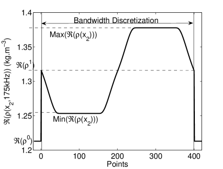
Figure 3: Real part of the density profile corresponding to $\rho^{1}(175kHz)$ chosen as the average value of $\rho(x_{2},175kHz)$ over $x_{2}\in[b,a]$.

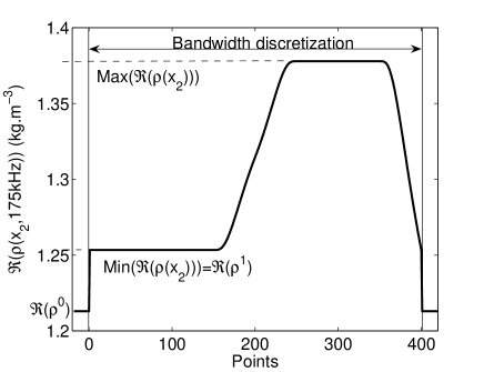
Figure 4: Real part of the density profile corresponding to $\rho^{1}(175kHz)$ chosen as the minimal value of $\rho(x_{2},175kHz)$ over $x_{2}\in[b,a]$.

To give an idea of the accuracy of the method, we introduce the following measure of the quadratic error, calculated for the $j$-th iteration:

$$E^{0^{+},j}=\frac{\int_{0}^{T}\left(p_{TMM}^{0^{+}d}(\mathbf{x},t)-p_{SGIM}^{0^{+}d,i}(\mathbf{x},t)\right)^{2}dt}{\int_{0}^{T}\left(p_{TMM}^{0^{+}d}(\mathbf{x},t)\right)^{2}dt}$$ (78)

wherein $p_{SGIM}^{0^{+}d}(\mathbf{x},t)$ is the reflected pressure as computed by our Specific Green’s Function based Iterative Scheme (SGIM), and $p_{TMM}^{0^{+}d}(\mathbf{x},t)$ the reflected pressure as computed by the classical Transfer Matrix Method (TMM), appendix C. The quadratic error corresponding to our computations is given figure 5.

Incidence angle of $\displaystyle 0$

Incidence angle of $\displaystyle\frac{\pi}{3}$

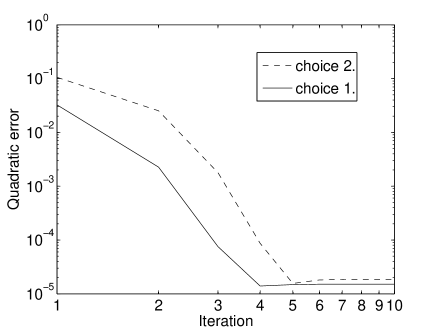
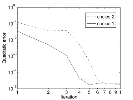
Figure 5: Evolution of the quadratic error as a function of the number of iterations. On the left: angle of incidence $\displaystyle 0$. On the right: $\displaystyle\frac{\pi}{3}$.

These experiments show that the correct choice of $\rho^{1}(\omega)$ and $k^{1}(\omega)$ is indeed to consider the average value of $\rho(x_{2},\omega)$ and $k(x_{2},\omega)$ over $x_{2}\in[b,a]$. This choice leads to a quicker and better convergence than the one obtained by the choice of $\rho^{1}(\omega)$ and $k^{1}(\omega)$ as the minimum of $\rho(x_{2},\omega)$ and $k(x_{2},\omega)$ over $x_{2}\in[b,a]$.

For both choices of these parameters, after a certain number of iterations, the SGIM results are the same as the classical TMM results, as shown figure 6, for example, when choice 1 is made.

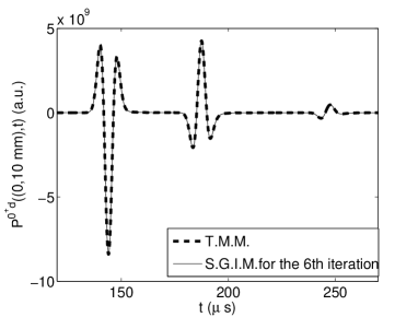
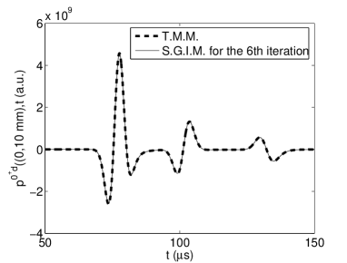
Figure 6: Reflected pressure as computed by the classical Transfer Matrix Method (TMM) -dashed curve- and as computed by our Specific Green’s Function based Iterative Method (SGIM) when choice 1. is made. The angle of incidence $\displaystyle 0$ on the left and $\displaystyle\frac{\pi}{3}$ on the right.

Remark: For both choices, $\displaystyle<\frac{1}{\rho}\frac{\partial\rho}{\partial x_{2}}>$, involved in the calculation of the first order Born approximation of both the reflected and transmitted fields, vanishes, i.e.,

$$<\frac{1}{\rho}\frac{\partial\rho}{\partial x_{2}}>=\int_{b}^{a}\frac{1}{\rho}\frac{\partial\rho}{\partial x_{2}}dx_{2}=\int_{b}^{a}\frac{\partial\ln\left(\rho(x_{2})\right)}{\partial x_{2}}dx_{2}=\ln\left(\frac{\rho(a)}{\rho(b)}\right)=0$$ (79)

because $\rho(x_{2})=\rho^{1}(\omega)$ for both $x_{2}=a$ and $x_{2}=b$.

Remark: Other choices are possible, such as the one leading to the disappearance of the averages $<\chi(x_{2})>$ involved in the calculation of the first order Born approximation of both the reflected and transmitted field. Consider $<\chi(x_{2})>$:

$$<\chi(x_{2})>=\int_{b}^{a}\left(\frac{(k(x_{2}))^{2}}{(k^{1})^{2}}-1\right)\frac{dx_{2}}{l}=\frac{1}{(k^{1})^{2}}\int_{b}^{a}(k(x_{2}))^{2}\frac{dx_{2}}{l}-1$$ (80)

which vanishes only if $\displaystyle k^{1}=\sqrt{\int_{b}^{a}(k(x_{2}))^{2}\frac{dx_{2}}{l}}$. This choice corresponds to the particular case in which $k(x_{2})$ is such that the Schwartz inequality is satisfied:

$$\left(\int_{b}^{a}k(x_{2})\frac{dx_{2}}{l}\right)^{2}\leq\int_{b}^{a}(k(x_{2}))^{2}\frac{dx_{2}}{l}~{}.$$ (81)

6 Results and discussion

We first present results, as calculated by the iterative scheme (FGIM) initialized with the zeroth-order Born approximation arising from the integral formulation incorporating the free-space Green’s function, to emphasize the fact that this method does not converge in all cases.

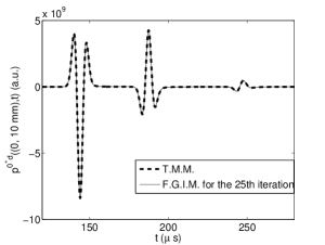
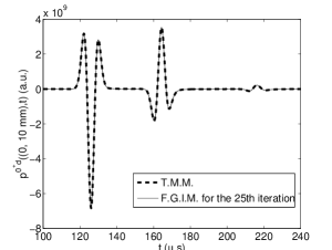
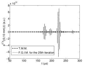
Figure 7: Reflected pressure as computed by the classical Transfert Matrix Method (TMM) and as computed by the classical free-space Green’s function based iterative scheme (FGIM). On the left : the incidence angle is $0$ ; in the middle : the incidence angle is $\displaystyle\frac{\pi}{6}$ and on the right : the incidence angle is $\displaystyle\frac{\pi}{3}$.

For small angles of incidence, the usual FGIM converges, figure 8 and 7, but slower and with less accuracy than our SGIM (figure 5). For large angles of incidence (in our example, $\displaystyle\frac{\pi}{3}$), the usual FGIM strongly diverges, figure 7, while our method still rapidly converges. This is probably caused by the fact that the first iteration is far from the exact solution (figure 8). The translation of this divergence can be appreciated in (figure 6).

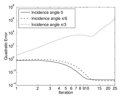
Figure 8: Evolution of the quadratic errors as a function of the number of iteration for various angles of incidence in the FGIM method.

All the following computations are carried out with characteristic parameters $\rho^{1}(\omega)$ and $k^{1}(\omega)$ filling the initially-homogeneous slab chosen as the average, over $a\leq x_{2}\leq b$, of $\rho(x_{2},\omega)$ and $k^{1}(x_{2},\omega)$ respectively.

We define a convergence criterion via the quadratic difference between two iterations $i$ and $j$ :

$$D_{i,j}=\frac{\int_{0}^{T}\left(p^{0^{+}d,i}(\mathbf{x},t)-p^{0^{+}d,j}(\mathbf{x},t)\right)^{2}dt}{\int_{0}^{T}\left(p^{0^{+}d,j}(\mathbf{x},t)\right)^{2}dt}~{}.$$ (82)

We found empirically that a convergence criterion $\mathcal{C}(i)$ of the form

$$\mathcal{C}(i)\mbox{ is true when }\frac{D_{i+1,i}}{D_{2,1}}\leq 1\times 10^{-6}$$ (83)

gives good results as shown figure 9 and 10. Our method yields solutions that are close to those of the usual TMM both in transmission and reflection in both the frequency and the time domain for several angles of incidence. This validates the method employing the SGF, combined with an iterative scheme initialized by a zeroth-order Born approximation.

The time history of the reflected pressure figure 9 is of particular interest for the demonstration of the accuracy of our method. We can clearly distinguish, for both angles of incidence $0$ and $\displaystyle\frac{\pi}{3}$, the three reflections of the incident wave on the three interfaces of our canonical configuration. The zeroth-order Born approximation, i.e. corresponding to the homogeneous fluid-saturated porous slab, formally accounts for two of them. For the first and third reflection, the amplitude matches correctly with our convergence criterion. The second reflection, which comes from the inhomogeneous slab, matches in both amplitude and time of arrival.

The time history of the transmitted pressure figure 10 contains only one peak due to the fact that absorption within the slab attenuates the transmitted waves resulting from multiple reflection.

Incidence angle of $\displaystyle 0$

Incidence angle of $\displaystyle\frac{\pi}{3}$

Convergence criterion

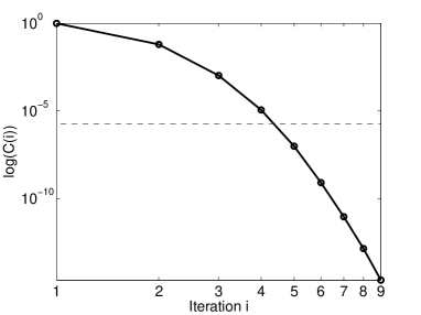
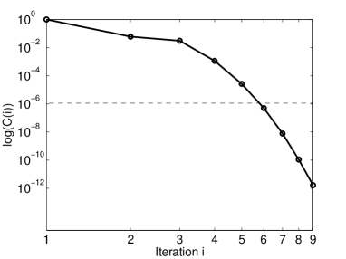
Reflected pressure

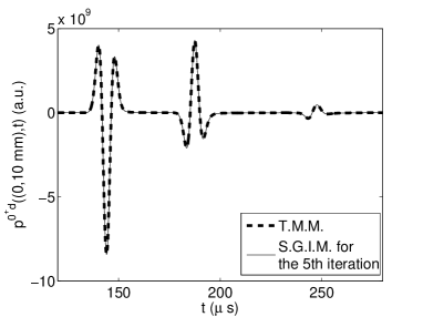
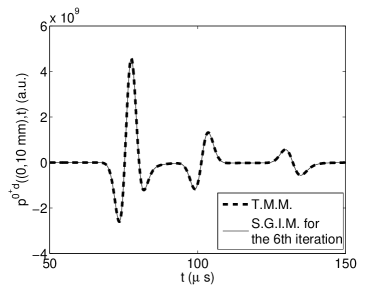
Spectrum

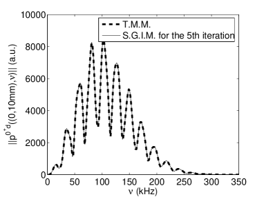
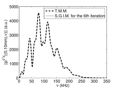
Figure 9: Reflected pressure. At the top: Convergence criterion; in the middle: the reflected pressure; at the bottom: the spectrum of the reflected pressure. On the left: incidence angle $=0$. On the right: incidence angle $\displaystyle=\frac{\pi}{3}$.

Incidence angle of $\displaystyle 0$

Incidence angle of $\displaystyle\frac{\pi}{3}$

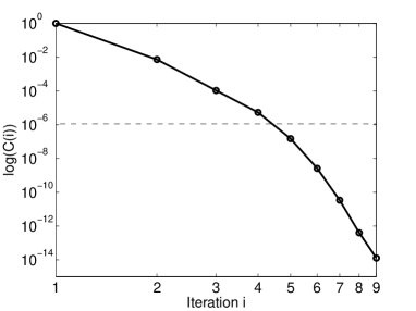
Convergence criterion

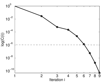
Transmitted pressure

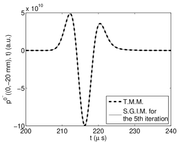
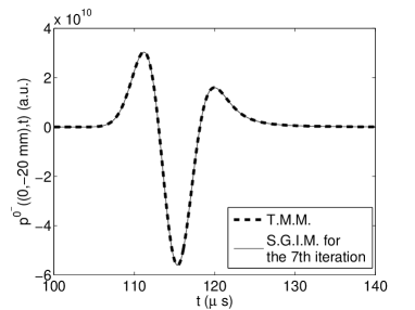
Spectrum

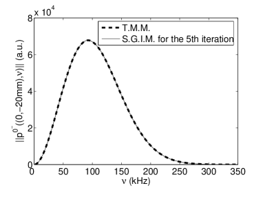
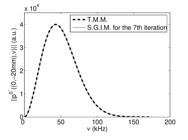
Figure 10: Transmitted pressure. At the top: Convergence criterion; in the middle: the transmitted pressure; at the bottom: the spectrum of the transmitted pressure. On the left: incidence angle $=0$. On the right: incidence angle $\displaystyle=\frac{\pi}{3}$.

7 Conclusion

A method, making use, in the domain integral formulation, of the specific Green’s function (SGF), i.e., the Green’s function of a canonical problem close to the original problem, for the resolution of problems of acoustic wave propagation in an inhomogeneous fluid medium (with spatially-varying density and compressibility) was studied and implemented for the canonical example of plane wave solicitation of a double layer fluid-saturated porous slab (considered as a single inhomogeneous slab) in the rigid frame (equivalent fluid) approximation.

A particular feature of our study is that we account for spatially-varying density, contrary to many authors who consider it to be constant. We also address the issue of the spatial differentiation of the pressure field at the boundaries of the inhomogeneity, which is carried by a finite-difference scheme for higher-than-zeroth-order Born approximations.

Our specific Green’s function iterative scheme, which is initialized by a zeroth-order Born approximation, was shown to converge, contrary to the iterative scheme relying on the free-space Green’s function, which is often found to be divergent. This improvement is due to the combined effects of the use of the SGF and to a better Born-like approximation of the field inside the heterogeneity.

In our numerical examples, our method was found to converge within 5-7 iterations to the reference solution (obtained rigorously by the transfer matrix method), even for an abrupt heterogeneity, and for various choices of the acoustic parameters filling the homogeneous slab supposed to be the initial configuration (canonical problem) for the SGF.

The robustness of the method was also demonstrated.

Our method thus appears useful for the resolution of inverse problems. In such a context, some information about the geometry and/or the mechanical properties of the objects one is looking for, is often known. The SGF is the device by which this information can be incorporated into the inversion procedure in a rational manner.

Appendix A The wave equation in an inhomogeneous fluid medium

A.1 Solution of the direct problem involving both the pressure and its partial derivative

Wave propagation, relative to an acoustic wave in an inhomogeneous fluid occupying a domain $\Omega=\Omega_{0}\cup\Omega_{1}$ (the homogeneous host medium occupies the domain $\Omega_{0}$ while the inhomogeneity occupies the domain $\Omega_{1}$), is described by:

$$\begin{array}[]{ll}\displaystyle\nabla\cdot\nabla p+\frac{\omega^{2}}{c(\mathbf{x})^{2}}-\frac{\nabla\rho(\mathbf{x})}{\rho(\mathbf{x})}\nabla p=\rho(\mathbf{x})s(\mathbf{x})&\displaystyle\mbox{; }\forall\mathbf{x}\in\Omega\end{array}$$ (84)

wherein: $\displaystyle c(\mathbf{x})=\sqrt{\frac{1}{\kappa(\mathbf{x})\rho(\mathbf{x})}}$ is the spatially-varying velocity, and $\kappa(\mathbf{x})$ and $\rho(\mathbf{x})$ the spatially-varying compressibility and density respectively of the fluid.

Applying the domain integral formulation with the usual free-space Green’s function, leads to the domain integral representation of the total field

$$p(\mathbf{y})=p^{i}(\mathbf{y})+\int_{\Omega_{1}}G^{0}\left(\mathbf{y},\mathbf{x}\right)\left(\left[\frac{\omega^{2}}{c(\mathbf{x})^{2}}-(k^{0})^{2}\right]p(\mathbf{y})-\frac{\nabla\rho(\mathbf{x})}{\rho(\mathbf{x})}\cdot\nabla p(\mathbf{x})\right)d\Omega(\mathbf{x})~{};~{}\forall\mathbf{y}\in\Omega$$ (85)

wherein $p^{i}(\mathbf{x})$ is the incident field. To obtain the field at an arbitrary point of space, $p$ and $\nabla p$ within $\Omega_{1}$ have to be determined. This can be done by solving the coupled system of integral equations:

$$\left\{\begin{array}[]{l}\displaystyle p(\mathbf{y})=p^{i}(\mathbf{y})+\int_{\Omega_{1}}G^{0}\left(\mathbf{y},\mathbf{x}\right)\left(\left[\frac{\omega^{2}}{c(\mathbf{x})^{2}}-(k^{0})^{2}\right]p(\mathbf{y})-\frac{\nabla\rho(\mathbf{x})}{\rho(\mathbf{x})}\cdot\nabla p(\mathbf{x})\right)d\Omega(\mathbf{x})~{};~{}\forall\mathbf{y}\Omega_{1}\\[10.0pt] \displaystyle\nabla_{\mathbf{y}}p(\mathbf{y})=\nabla_{\mathbf{y}}p^{i}(\mathbf{y})+\int_{\Omega_{1}}\nabla_{\mathbf{y}}G^{0}\left(\mathbf{y},\mathbf{x}\right)\left(\left[\frac{\omega^{2}}{c(\mathbf{x})^{2}}-(k^{0})^{2}\right]p(\mathbf{y})-\frac{\nabla\rho(\mathbf{x})}{\rho(\mathbf{x})}\cdot\nabla p(\mathbf{x})\right)d\Omega(\mathbf{x})~{};~{}\forall\mathbf{y}\Omega_{1}\end{array}\right.$$ (86)

A vast literature exists on the subject of the numerical resolution of systems of domain integral equations [21, 29, 34, 16, 6, 45].

A.2 Solving the direct problem via a single integral equation

Another, perhaps simpler (although unsuitable in the inverse problem context) way, to solve the previous problem is to make the substitution

$$p(\mathbf{x})=q(\mathbf{x})\sqrt{\rho(\mathbf{x})}$$ (87)

whereby the following governing equation is obtained

$$\nabla^{2}q(\mathbf{x})+\left[\frac{\omega^{2}}{c(\mathbf{x})^{2}}+\frac{1}{2}\frac{\nabla^{2}\rho(\mathbf{x})}{\rho(\mathbf{x})}-\frac{3}{4}\frac{\nabla\rho(\mathbf{x})\cdot\nabla\rho(\mathbf{x})}{\left(\rho(\mathbf{x})\right)^{2}}\right]q(\mathbf{x})=\rho^{\frac{1}{2}}(\mathbf{x})s(\mathbf{x})\mbox{ ; }\mathbf{x}\in\Omega~{}.$$ (88)

Using the free-space Green’s function in the domain integral formulation yields the representation

$$q(\mathbf{y})=q^{i}(\mathbf{y})+\\ \int_{\Omega_{1}}G^{0}\left(\mathbf{y},\mathbf{x}\right)\left[\frac{\omega^{2}}{\left(c(\mathbf{x})\right)^{2}}-\left(k^{0}\right)^{2}+\frac{1}{2}\frac{\nabla\cdot\nabla\rho(\mathbf{x})}{\rho(\mathbf{x})}-\frac{3}{4}\frac{\nabla\rho(\mathbf{x})\cdot\nabla\rho(\mathbf{x})}{\left(\rho(\mathbf{x})\right)^{2}}\right]q(\mathbf{x})dv(\mathbf{x})\mbox{ ; }\forall\mathbf{y}\in\Omega,$$ (89)

from which is extracted a single integral equation for $q(\mathbf{x})~{};~{}\mathbf{x}\in\Omega_{1}$.

Remark: The integral formulations (86) and (89) are identical when the density is constant.

A.3 A canonical problem involving a density discontinuity.

Let us consider the simple $1D$ problem, depicted in figure 11, of a plane wave striking a planar interface $\Gamma$, located at $x_{2}=a$, between two homogeneous media $\Omega_{0}$ and $\Omega_{1}$. The normally-incident plane wave travels initially in $\Omega_{0}$. The heterogeneity is supposed to be the domain $\Omega_{1}$.

In practice, this problem can be treated rigorously by the TMM method. However, when one attempts to solve it by the integral method, the medium filling $\Omega_{1}$ must be dissipiative.

Let us suppose that the pressure field $p^{1}$ in $\Omega_{1}$ is known (for example, calculated by the TMM method).

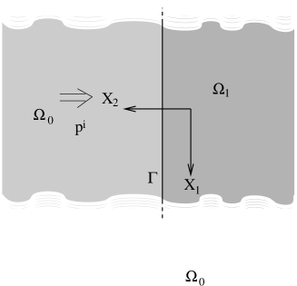
Figure 11: Configuration of a planar interface between two domains.

We introduce $\rho(x_{2})=\rho^{1}+\left(\rho^{0}-\rho^{1}\right)H(x_{2})$ and $k(x)=k^{1}+\left(k^{0}-k^{1}\right)H(x_{2})$, where $H(x_{2})$ is the Heaviside function, and $k^{j}$, $j=0,1$ the wavenumber in the domain $\Omega_{j}$.

Eq. (85) splits into:

$$p(y_{2})=p^{i}(y_{2})+\int_{-\infty}^{a}G^{0}\left(y_{2},x_{2}\right)\left(k^{1}\right)^{2}p(\mathbf{y})dx_{2}-\left(\rho^{0}-\rho^{1}\right)\int_{-\infty}^{a}\frac{\delta(x_{2}-a)}{\rho(x_{2})}\frac{\partial p(x_{2})}{\partial x_{2}}dx_{2},\forall\mathbf{y}\Omega$$ (90)

wherein $\delta$ is the Dirac delta distribution. All the integrals involved in (90) can be solved analytically ($p(x_{2})$ begin known by hypothesis). In particular, the function $\displaystyle\frac{1}{\rho(x_{2})}\frac{\partial p(x_{2})}{\partial x_{2}}$ is continuous (i.e. the function is $C^{0}$) at the interface $\Gamma$ so that the second integral does not present any difficulties.

The formulation involving the evaluation of $p$ and of $\nabla p$ allows us to take into account density discontinuities. Eq. (89) splits into

$$q(y_{2})=q^{i}(y_{2})+\int_{-\infty}^{a}G^{0}\left(y_{2},x_{2}\right)\left(k^{1}\right)^{2}q(x_{2})dx_{2}+\\ \frac{\left(\rho^{0}-\rho^{1}\right)}{2}\int_{-\infty}^{a}\frac{\delta^{\prime}(x_{2}-a)}{\rho(x_{2})}q(x_{2})dx_{2}-\\ \frac{3\left(\rho^{0}-\rho^{1}\right)^{2}}{4}\int_{-\infty}^{a}\frac{\delta(x_{2}-a)\delta(x_{2}-a)}{\left(\rho(\mathbf{x})\right)^{2}}q(x_{2})dx_{2}\mbox{ ; }\forall y_{2}\in\Omega~{}.$$ (91)

The calculation of first integral presents no particular difficulties. Let us consider the second integral $\displaystyle\int_{-\infty}^{a}\frac{\delta^{\prime}(x_{2}-a)}{\rho(x_{2})}q(x_{2})dx_{2}$, wherein $\delta^{\prime}(x_{2}-a)$ is the derivative of the Dirac delta distribution. The use of the formula

$$\int f(x_{2})\delta^{\prime}(x_{2}-a)dx_{2}=-\frac{\partial f(x_{2})}{\partial x_{2}}\delta(x_{2}-a)$$ (92)

requires the function $f(x_{2})$ to be $C^{1}$ at $x_{2}=a$, while the function $\displaystyle\frac{q(x_{2})}{\rho(x_{2})}=\frac{p(x_{2})}{\rho(x_{2})^{\frac{3}{2}}}$ is not continuous at the interface $\Gamma$. Thus, this second term cannot be handled analytically.

Finally, consider the third term $\displaystyle\int_{-\infty}^{a}\frac{\delta(x_{2}-a)\delta(x_{2}-a)}{\left(\rho(\mathbf{x})\right)^{2}}q(x_{2})dx_{2}$. The integrand involves the scalar product of two Dirac delta distributions $\delta(x_{2}-a)\delta(x_{2}-a)$ which is not defined [31, 15, 14]. A Numerical approximation of this quantity exists, but otherwise it is meaningless [14].

The resolution of problems via a single equation is also of no practical use when the problem one is faced with involves density discontinuities.

Appendix B Pressure field in the case of a macroscopically-homogeneous porous slab (zeroth-order Born approximation).

By referring to [18], one finds, that for plane wave solicitation in $\Omega_{0}^{+}$, the pressure fields in $\Omega_{0}^{-}$, $\Omega_{1}$ and $\Omega_{0}^{+}$ are:

$$p^{0+}(\mathbf{x},\omega)=A^{i}(\omega)\exp\left(\mbox{i}k_{1}^{i}x_{1}-\mbox{i}k_{2}^{0,i}x_{2}\right)+\\ A^{i}(\omega)\frac{\mbox{i}\exp\left(\mbox{i}k_{1}^{i}x_{1}+\mbox{i}k_{2}^{0,i}(x_{2}-2a)\right)\sin\left(k_{2}^{1,i}l\right)\left((\alpha^{1,i})^{2}-(\alpha^{0,i})^{2}\right)}{2\alpha^{1,i}\alpha^{0,i}\cos\left(k_{2}^{1,i}l\right)-\mbox{i}\left((\alpha^{1,i})^{2}+(\alpha^{0,i})^{2}\right)\sin\left(k_{2}^{1,i}l\right)}=\exp\left(\mbox{i}k_{1}^{i}x_{1}\right)\widetilde{p}^{0-}(x_{2},\omega)$$ (93)

$$p^{1}(\mathbf{x},\omega)=A^{i}(\omega)\frac{2\exp\left(\mbox{i}k_{1}^{i}x_{1}-\mbox{i}k_{2}^{0,i}a\right)\alpha^{0,i}\left[\alpha^{1,i}\cos\left(k_{2}^{1,i}(x_{2}-b)\right)-\mbox{i}\alpha^{0,i}\sin\left(k_{2}^{1,i}(x_{2}-b)\right)\right]}{2\alpha^{1,i}\alpha^{0,i}\cos\left(k_{2}^{1,i}l\right)-\mbox{i}\left((\alpha^{1,i})^{2}+(\alpha^{0,i})^{2}\right)\sin\left(k_{2}^{1,i}l\right)}=\\ \exp\left(\mbox{i}k_{1}^{i}x_{1}\right)\widetilde{p}^{1}(x_{2},\omega)$$ (94)

$$\frac{\partial p^{1}(\mathbf{x},\omega)}{\partial x_{2}}=A^{i}(\omega)\frac{2\exp\left(\mbox{i}k_{1}^{i}x_{1}-\mbox{i}k_{2}^{0,i}a\right)\alpha^{0,i}k_{2}^{1,i}\left[-\alpha^{1,i}\sin\left(k_{2}^{1,i}(x_{2}-b)\right)-\mbox{i}\alpha^{0,i}\cos\left(k_{2}^{1,i}(x_{2}-b)\right)\right]}{2\alpha^{1,i}\alpha^{0,i}\cos\left(k_{2}^{1,i}l\right)-\mbox{i}\left((\alpha^{1,i})^{2}+(\alpha^{0,i})^{2}\right)\sin\left(k_{2}^{1,i}l\right)}=\\ \exp\left(\mbox{i}k_{1}^{i}x_{1}\right)\frac{\partial\widetilde{p}^{1}(x_{2},\omega)}{\partial x_{2}}$$ (95)

$$p^{0-}(\mathbf{x},\omega)=A^{i}(\omega)\frac{2\exp\left(\mbox{i}k_{1}^{i}x_{1}-\mbox{i}k_{2}^{0,i}\left(x_{2}+l\right)\right)\alpha^{1,i}\alpha^{0,i}}{2\alpha^{1,i}\alpha^{0,i}\cos\left(k_{2}^{1,i}l\right)-\mbox{i}\left((\alpha^{1,i})^{2}+(\alpha^{0,i})^{2}\right)\sin\left(k_{2}^{1,i}l\right)}=\exp\left(\mbox{i}k_{1}^{i}x_{1}\right)\widetilde{p}^{0-}(x_{2},\omega)~{}.$$ (96)

Appendix C Pressure field in the case of a double layer macroscopically-homogeneous porous slabs.

We use a separation of variables technique to obtain the field representations:

$$\begin{array}[]{l}\displaystyle p^{0^{+}}=A^{i}(\omega)e^{\mbox{i}[k_{1}^{i}x_{1}-k_{2}^{0,i}x_{2}]}+B^{0^{+}}e^{\mbox{i}[k_{1}^{i}x_{1}+k_{2}^{0,i}\left(x_{2}-a\right)]}\\[8.0pt] \displaystyle p^{1}=e^{\mbox{i}k_{1}^{i}x_{1}}\left(A^{1}e^{-\mbox{i}k_{2}^{1,i}\left(x_{2}-a\right)}+B^{1}e^{\mbox{i}k_{2}^{1,i}\left(x_{2}-a\right)}\right)\\[8.0pt] \displaystyle p^{2}=e^{\mbox{i}k_{1}^{i}x_{1}}\left(A^{2}e^{-\mbox{i}k_{2}^{2,i}\left(x_{2}-b\right)}+B^{2}e^{\mbox{i}k_{2}^{2,i}\left(x_{2}-b\right)}\right)\\[8.0pt] \displaystyle p^{0^{-}}=A^{0^{-}}e^{\mbox{i}[k_{1}^{i}x_{1}-k_{2}^{0,i}\left(x_{2}-b\right)]}\end{array}$$ (97)

After introducing the fields expressions into the boundary conditions (continuity of the pressure and of the normal velocity), we multiply these relations by $\exp\left(-\mathbf{i}K_{1}x_{1}\right)$ and then integrate form $-\infty$ to $+\infty$ to obtain the matrix equation (solved numerically to get $B^{0^{+}}$ and $A^{0^{-}}$)

$$\left(\!\begin{array}[]{llllll}\displaystyle 1&\displaystyle-1&\displaystyle-1&\displaystyle 0&\displaystyle 0&\displaystyle 0\\[8.0pt] \displaystyle\alpha^{0,i}&\displaystyle\alpha^{1,i}&\displaystyle-\alpha^{1,i}&\displaystyle 0&\displaystyle 0&\displaystyle 0\\[8.0pt] \displaystyle 0&\displaystyle e^{\mbox{i}k_{2}^{1,i}l^{1}}&\displaystyle e^{-\mbox{i}k_{2}^{1,i}l^{1}}&\displaystyle-e^{-\mbox{i}k_{2}^{2,i}l^{2}}&\displaystyle-e^{\mbox{i}k_{2}^{2,i}l^{2}}&\displaystyle 0\\[8.0pt] \displaystyle 0&\displaystyle-\alpha^{1,i}e^{\mbox{i}k_{2}^{1,i}l^{1}}&\displaystyle\alpha^{1,i}e^{-\mbox{i}k_{2}^{1,i}l^{1}}&\displaystyle\alpha^{2,i}e^{-\mbox{i}k_{2}^{2,i}l^{2}}&\displaystyle-\alpha^{2,i}e^{\mbox{i}k_{2}^{2,i}l^{2}}&\displaystyle 0\\[8.0pt] \displaystyle 0&\displaystyle 0&\displaystyle 0&\displaystyle 1&\displaystyle 1&\displaystyle-1\\[8.0pt] \displaystyle 0&\displaystyle 0&\displaystyle 0&\displaystyle-\alpha^{2,i}&\displaystyle\alpha^{2,i}&\displaystyle\alpha^{0,i}\\[8.0pt] \end{array}\!\right)\!\left(\!\begin{array}[]{l}\displaystyle\!B^{0^{+}}\!\\[8.0pt] \displaystyle\!A^{1}\!\\[8.0pt] \displaystyle\!B^{1}\!\\[8.0pt] \displaystyle\!A^{2}\!\\[8.0pt] \displaystyle\!B^{2}\!\\[8.0pt] \displaystyle\!A^{0^{-}}\!\\[8.0pt] \end{array}\!\right)\!=\!\left(\!\begin{array}[]{l}\displaystyle\!-A^{i}(\omega)e^{-\mbox{i}k_{2}^{0,i}a}\!\\[8.0pt] \displaystyle\!\alpha^{0,i}A^{i}(\omega)e^{-\mbox{i}k_{2}^{0,i}a}\!\\[8.0pt] \displaystyle 0\\[8.0pt] \displaystyle 0\\[8.0pt] \displaystyle 0\\[8.0pt] \displaystyle 0\\[8.0pt] \end{array}\!\right)$$ (98)

wherein $l^{1}$ and $l^{2}$ are the thickness of the layer 1 and the layer 2 respectively (table 1) and $\displaystyle\alpha^{j,i}=\frac{k_{2}^{j,i}}{\rho^{j}}$, $j=0^{+},1,2,0^{-}$.

References

- 1. K. Aki and P.G. Richards. Quantitative Seismology. Freeman, San Francisco, 1980.
- 2. T. Aktosun and M. Klaus. Inverse theory: problem on the line. In R. Pike and P. Sabatier, editors, Scattering, pages 770–785, San Diego, 2002. Academic Press.
- 3. J.-F. Allard and Y. Champoux. New empirical equations for sound propagation in rigid frame porous materials. J.Acoust.Soc.Am., 91:3346–3353, 1992.
- 4. J.F. Allard. Propagation of Sound in Porous Media: Modeling Sound Absorbing Materials. Chapman and Hall, London, 1993.
- 5. Z. Alterman. Finite difference solutions to geophysical problems. J.Phys.Earth., 16:113–128, 1968.
- 6. K.E. Atkinson. The Numerical Solution of Integral Equations of the Second Kind. Cambridge Univ. Press, Cambridge, 1997.
- 7. C. Boutin, P. Royer, and J.-L. Auriault. Acoustic absorption of porous surfacing with dual porosity. Int.J.Solids Struct., 35:4709–4737, 1998.
- 8. L.M. Brekhovskikh. Waves in Layered Media. Academic Press, New York, 1960.
- 9. L.M. Brekhovskikh and Y. Lysanov. Fundamentals of Ocean Acoustics. Springer, Berlin, 1991.
- 10. J. Buchanan, R. Gilbert, A. Wirgin, and Y. Xu. Transient reflection and transmission of ultrasonic waves in cancellous bone. Appl.Math. & Computation, 142:561–573, 2003.
- 11. J.L. Buchanan and R.P. Gilbert. Transmission loss in a shallow ocean over a two-layer seabed. Int.J.Solids Struct., 35:4779–4801, 1998.
- 12. J.L. Buchanan, R.P. Gilbert, A. Wirgin, and Y. Xu. Marine Acoustics: Direct and Inverse Problems. SIAM, Philadelphia, 2004.
- 13. L.A. Chernov. Wave propagation in a Random Medium. Mc Graw-Hill, New-York, 1960.
- 14. J.F. Colombeau. New Generalized Functions and Multiplication of Distributions. North-holland, Amsterdam, 1984.
- 15. J.F. Colombeau. Lecture notes in Mathematics, chapter Multiplication of Distributions (A Tool in Mathematics, Numerical Engineering and Theoretical Physics). Spinger-Verlag, 1992.
- 16. D. Colton and R. Kress. Integral Equation Methods in Scattering Theory. Wiley, New-York, 1983.
- 17. L. De Ryck, J.-P. Groby, P. Leclaire, W. Lauriks, A. Wirgin, C. Depollier, and Z.E.A. Fellah. Acoustic wave propagation in a macroscopically inhomogeneous porous medium saturated by a fluid. submitted to Phys.Rev.Lett., 2006.
- 18. J.-P. Groby, E. Ogam, A. Wirgin, Z.E.A. Fellah, W. Lauriks, J.-Y. Chapelon, C. Depollier, L. De Ryck, R. Gilbert, N. Sebaa, and Y. Xu. 2d mode excitation in a porous slab saturated with air in the high frequency approximation. In Symposium on the Acoustics of Poro-Elastic Materials, pages 53–60, ENTPE, Lyon, France, December 7-8-9 2005.
- 19. J.-P. Groby and C. Tsogka. A time domain method to model viscoacoustic and viscoelastic sh wave propagation. In G.C. Cohen and E. Heikkola, editors, Mathematical and Numerical Aspects of Wave Propagation WAVES 2003, pages 911–915, Berlin, 2003. Springer.
- 20. R. Haḧner. Scattering by media. In R. Pike and P. Sabatier, editors, Scattering, pages 75–94, San Diego, 2002. Academic Press.
- 21. R.F. Harrington. Field Computation by Moment Methods. IEEE Press, New-York, 1993.
- 22. K.A.H. Innanen. Methods for the treatment of acoustic and absorptive/dispersive wave field measurements. PhD thesis, University of British Columbia, 2004.
- 23. A. Ishimaru. Wave Propagation and Scatterng in Random Media. Academic Press, New York, 1978.
- 24. D. J. Johnson, J. Koplik, and R. Dashen. Theory of dynamic permeability and tortuosity in fluid-saturated porous media. J.Fluid.Mech., 176:379–402, 1987.
- 25. D. Jongmans, D. Demanet, C. Horrent, M. Campillo, and F.J. Sanchez-Sesma. Dynamic soil parameters determination by geophysical prospecting in mexico city: implication for site effect modeling. Soil Dynam.Earthquake Engrg., 15:549–559, 1996.
- 26. A.C. Kak and M. Slaney. Principles of Computerized Tomographic Imaging. IEEE Press, New-Yor, 1999.
- 27. J.B. Keller. Accuracy and validity of the born and rytov approximations. J.Opt.Soc.Am., 59:1003–1004, 1969.
- 28. L. Knopoff. A matrix method for elastic wave problems. Bull.Seism.Soc.Am., 54:431–438, 1964.
- 29. R. Kress. Linear Integral Equations. Springer, 1989.
- 30. G. Kristensson, A. Karlsson, and S. Rikte. Electromagnetic wave propagation in dispersive and complex material with time-domain techniques. In R. Pike and P. Sabatier, editors, Scattering, pages 277–294, San Diego, 2002. Academic Press.
- 31. P. Kurasov. Distribution theory for discontinuous test functions and differential operators with generalized coefficients. J.Math.Anal.Appl., 201:297–323, 1996.
- 32. M. Lambert, R. de Oliveira Bohbot, and D. Lesselier. Reconstruction des paramètres acoustiques d’un fond marin stratifié à partir de son coefficient de réflexion. J.Phys. IV, Coll. C1, supp. J.Phys.III, 2:945–948, 1992.
- 33. J. Lundstedt and M. Norgren. Comparison between frequency domain and time domain methods for parameter reconstruction on nonuniform dispersive transmission lines. Progress In Electromagnetics Research, 43:1–37, 2003.
- 34. S.G. Mikhlin and K.L. Smotitskiy. Approximated Methods for Solution of Differential and Intergal Equations. Elsevier, New-York, 1967.
- 35. P.M. Morse and K.U. Ingard. Theoretical Acoustics. Princeton Universty Press, Princeton, 1986.
- 36. W. Munk, P.F. Worcester, and C. Wunsch. Ocean Acoustic Tomography. Cambridge University Press, Cambridge, 1995.
- 37. R.G. Newton. Three-dimensional direct scattering theory. In R. Pike and P. Sabatier, editors, Scattering, pages 686–701, San Diego, 2002. Academic Press.
- 38. P. Sabatier. Past and future of inverse problems. J.Math.Phys., 41:4082–4124, 2000.
- 39. P. Sabatier. Approximate methods in scattering. In R. Pike and P. Sabatier, editors, Scattering, pages 717–725, San Diego, 2002. Academic Press.
- 40. J.A. Scales. Imaging and inversion with acoustic and elastic waves. In R. Pike and P. Sabatier, editors, Scattering, pages 578–593, San Diego, 2002. Academic Press.
- 41. D.R Smith, W.J. Padilla, D.C. Vier, S.C. Nemat-Nasser, and S. Schultz. Composite medium with simultaneously negative permeability and permittivity. Phys.Rev.Lett., 84:4184–4187, 2000.
- 42. R. Snieder. Wavefield Inversion, chapter Inverse problems in geophysics. Springer, Vienna, 1999.
- 43. A.G. Tijhuis, K. Belkebir, A.C.S Litman, and B.P. de Hon. Theoretical and computational aspects of 2-d inverse profiling. IEEE Trans.Geosc.Rem.Sens., 39:1316–1330, 2001.
- 44. C.P.A. Wapenaar. Inversion versus migration: a new perspective to an old discussion. Geophys., 61:804–814, 1996.
- 45. A. Wirgin. Wavefield Inversion, chapter Some quasi-analytic and numerical methods for acoustical imaging of complex media, pages 241–304. Springer, Wien, 1999.
- 46. A. Wirgin. Méthodes d’identification approchée de cibles sondées par ondes impulsives. HAL/CCSD/CEL-26/09/05, 2005.
- 47. E. Yablonovitch. Photonic crystals. J. Mod.Opt., 41:173–194, 1994.
- 48. X. Zhu and G.A. Mc Mechan. Numerical simulation of seismic responses of poroelastic reservoirs using biot theory. Geophys., 56:328–339, 1991.