A Stochastic Evolutionary Growth Model for Social Networks

Abstract

We present a stochastic model for a social network, where new actors may join the network, existing actors may become inactive and, at a later stage, reactivate themselves. Our model captures the evolution of the network, assuming that actors attain new relations or become active according to the preferential attachment rule. We derive the mean-field equations for this stochastic model and show that, asymptotically, the distribution of actors obeys a power-law distribution. In particular, the model applies to social networks such as wireless local area networks, where users connect to access-points, and peer-to-peer networks where users connect to each other. As a proof of concept, we demonstrate the validity of our model empirically by analysing a public log containing traces from a wireless network at Dartmouth College over a period of three years. Analysing the data processed according to our model, we demonstrate that the distribution of user accesses is asymptotically a power-law distribution.

1 Introduction

We present a stochastic model for a social network [Sco00], where new actors may join the network, existing actors may become inactive and, at a later stage, may reactivate themselves. Our model captures the evolution of the network, assuming that actors attain new relations or become active according to the preferential attachment rule. The concept of preferential attachment, originating from [Pri76], has become a common theme in stochastic models of networks [AB02, New03]. This behaviour often results in the “rich get richer” phenomenon, for example, where new relations to existing actors are formed in proportion to the number of relations those actors currently have.

The model presented incorporates the novel aspect of differentiating between active and inactive actors, and allowing actors’ status to change between active and inactive over time. This type of network dynamics is especially relevant to situations where actors may connect/disconnet or login/logout from the network, in particular, when network registration is needed as a prior condition to the first time an actor connects to the network. The network models proposed so far either assume that all actors are active, or that when actors leave the network they do not rejoin it [ASBS00].

By deriving the mean-field equations for this model of a social network, we obtain the result that, asymptotically, the distribution of actors obeys a power law. Power-law distributions taking the form

$$f(i)=C\ i^{-\phi},$$

where $C$ and $\phi$ are positive constants, are abundant in nature [Sch91]. The constant $\phi$ is called the exponent of the distribution. Examples of such distributions are: Zipf’s law, which states that the relative frequency of a word in a text is inversely proportional to its rank, Pareto’s law, which states that the number of people whose personal income is above a certain level follows a power-law distribution with an exponent between 1.5 and 2 (Pareto’s law is also known as the 80:20 law, stating that about 20% of the population earn 80% of the income) and Lotka’s law, which states that the number of authors publishing a prescribed number of papers is inversely proportional to the square of the number of publications.

Recently, several researchers have detected power-law distributions in the topology of several networks such as the World-Wide-Web [BKM⁺00], e-mail networks [EMB02], collaboration networks [Gro02, FLL06] and peer-to-peer networks [RIF02].

There are several examples of networks that can be modelled within our formalism. One example is that of a wireless network [KE05], where mobile users having, e.g. a laptop, PDA or mobile phone, connect to access points within a defined region (e.g. campus, building or airport). In this case the actors are the users and the relations are between users and access points. The user is active during a connection and otherwise inactive. Another example, is that of a peer-to-peer network [Ora01], where users (referred to as peers) connect to other peers in order to exchange information. Peer-to-peer networks are of prime importance to the future of the internet, as networks such as Bittorrent [PGES05], Kazaa [LKR06] and Skype [GDJ06] are becoming increasingly popular and thus account for a sizeable amount of all internet traffic.

Our stochastic model is based on the transfer of balls (representing actors) between urns (representing actor states), where we distinguish between active balls in, regular, unstarred urns and inactive balls in starred urns. The relationships of a particular actor are represented as pins attached to the corresponding ball.

We note that our urn model is an extension of the stochastic model proposed by Simon in his visionary paper published in 1955 [Sim55], which was couched in terms of word frequencies in a text. Previously, in [FLL06], we considered an alternative extension of Simon’s model by adding a preferential mechanism for discarding balls from urns resulting in an exponential cutoff in the power-law distribution.

In the model we present here, at each step of the stochastic process, with probability $p$, two events may happen: either a new active ball is added to the first unstarred urn with probability $r$, or with probability $1-r$ an inactive ball is selected preferentially from a starred urn and is activated by moving it to the corresponding unstarred urn. Alternatively, with probability $1-p$, an active ball is selected preferentially from an unstarred urn and then two further events may happen: it is either moved along to the next unstarred urn with probability $q$, or with probability $1-q$ the selected ball becomes inactive by moving it to the corresponding starred urn. We assume that a ball in the $i$th urn has $i$ pins attached to it (which represents an actor having $i$ relations). Our main result is that the steady-state distribution of this model is an asymptotic power law, and, moreover, as a proof of concept we demonstrate the validity of our model by analysing data from a real wireless network.

The rest of the paper is organised as follows. In Section 2 we present an urn transfer model allowing balls to be active or inactive by moving from starred urns to unstarred urns and vice versa. We then derive in Section 3 the steady-state distribution of the model, which, as stated earlier, follows an asymptotic power-law distribution. In Section 4 we show how we can fit the parameters of the model to data, and in Section 5 we demonstrate how our model can provide an explanation of the empirical distributions found in wireless networks. Finally, in Section 6 we give our concluding remarks.

2 An Urn Transfer Model

We now present an urn transfer model for a stochastic process that emulates the situation where balls (which might represent actors) become inactive with a small probability, and can later become active again with some probability. We assume that a ball in the $i$th urn has $i$ pins attached to it (which might represent the actors’ relations). The model is an extension of our previous model of exponential cutoff [FLL05], where balls are discarded with a small probability.

We assume a countable number of (unstarred) urns, $urn_{1},urn_{2},urn_{3},\ldots\$ and correspondingly a countable number of starred urns $urn^{*}_{1},urn^{*}_{2},urn^{*}_{3},\ldots\$, where the former contains active balls and the latter contain the inactive balls. Initially all of the urns are empty except $urn_{1}$, which has one ball in it. Let $F_{i}(k)$ and $F^{*}_{i}(k)$ be the number of balls in $urn_{i}$ and $urn^{*}_{i}$, respectively, at stage $k$ of the stochastic process, so $F_{1}(1)=1$, all other $F_{i}(1)=0$ and all $F^{*}_{i}(1)=0$. Then, at stage $k+1$ of the stochastic process, where $k\geq 1$, one of two events may occur:

1. with probability $p$, $0<p<1$, one of two events may happen:

   1. with probability $r$, $0<r\leq 1$, a new ball (with one pin attached to it) is inserted into $urn_{1}$, or

   2. with probability $1-r$, a starred urn is selected, with $urn^{*}_{i}$ being selected with probability proportional to $iF^{*}_{i}(k)$, the number of pins it contains, and a ball is chosen from the selected urn, $urn^{*}_{i}$, and transferred to $urn_{i}$ (this is equivalent to making the ball active).

2. with probability $1-p$ an urn is selected, with $urn_{i}$ being selected with probability proportional to $iF_{i}(k)$, the number of pins it contains, and a ball is chosen from the selected urn, $urn_{i}$; then,

   1. with probability $q$, $0<q\leq 1$, the chosen ball is transferred to $urn_{i+1}$, (this is equivalent to attaching an additional pin to the ball chosen from $urn_{i}$), or

   2. with probability $1-q$ the ball chosen is transferred to $urn^{*}_{i}$ (this is equivalent to making the ball inactive).

We note that we could modify the initial conditions so that, for example, $urn_{1}$ and $urn^{*}_{1}$ initially contained $\delta,\delta^{*}>1$ balls, respectively, instead of $urn_{1}$ having just one ball and $urn^{*}_{1}$ being empty. It can be shown, from the development of the model below, that any change in the initial conditions will have no effect on the asymptotic distribution of the balls in the urns as $k$ tends to infinity, provided the process does not terminate with either all of the unstarred urns empty or all of the starred urns empty (cf. [FLL05]). In the former case we need to ensure that $p>(1-p)(1-q)$, i.e. that the number of balls going into unstarred urns is greater than the number of balls going out of unstarred urns. In the latter case we need to ensure that $(1-p)(1-q)>p(1-r)$, i.e. that the number of balls going into starred urns is greater than the number of balls going out of starred urns.

More specifically, the probability of termination must be small, i.e.

$$\left(\frac{(1-p)(1-q)}{p}\right)^{\delta}<\epsilon$$

and

$$\left(\frac{p(1-r)}{(1-p)(1-q)}\right)^{\delta^{*}}<\epsilon$$

for some $\epsilon>0$. We observe that these are the probabilities that the gambler’s fortune will not increase forever [Ros83].

The expected total number of balls in the unstarred urns at stage $k$ is given by

$$E\Big{(}\sum_{i=1}^{k}F_{i}(k)\Big{)} = 1+(k-1)\Big{(}p-(1-p)(1-q)\Big{)}$$ (1)

$$= (1-p)(2-q)+k\Big{(}p-(1-p)(1-q)\Big{)},$$

and in the starred urns by

$$E\Big{(}\sum_{i=1}^{k}F^{*}_{i}(k)\Big{)} = (k-1)\Big{(}(1-p)(1-q)-p(1-r)\Big{)}.$$ (2)

The total number of pins attached to balls in $urn_{i}$ at stage $k$ is $iF_{i}(k)$, so the expected total number of pins in the unstarred urns is given by

$$E\Big{(}\sum_{i=1}^{k}iF_{i}(k)\Big{)} = 1+(k-1)\Big{(}rp+(1-p)q\Big{)}+p(1-r)\sum_{j=1}^{k-1}\psi_{j}-(1-p)(1-q)\sum_{j=1}^{k-1}\theta_{j},$$ (3)

where $\psi_{j}$, $1\leq j\leq k-1$, is the expectation of $\Psi_{j}^{\prime}$, the number of pins attached to the ball chosen at step (ib) of stage $j+1$ (i.e. the urn number), and $\theta_{j}$, $1\leq j\leq k-1$, is the expectation of $\Theta_{j}^{\prime}$, the number of pins attached to the ball chosen at step (iib) of stage $j+1$ (i.e. the urn number). More specifically,

$$\psi_{j}=E(\Psi_{j}^{\prime})=E\left(\frac{\sum_{i=1}^{j}i^{2}F^{*}_{i}(j)}{\sum_{i=1}^{j}iF^{*}_{i}(j)}\right)$$ (4)

and

$$\theta_{j}=E(\Theta_{j}^{\prime})=E\left(\frac{\sum_{i=1}^{j}i^{2}F_{i}(j)}{\sum_{i=1}^{j}iF_{i}(j)}\right).$$ (5)

The quotient of sums in the second expectation in (4) (respectively in (5)), which we denote by $\Psi_{j}$ (respectively by $\Theta_{j}$), is the expected value of $\Psi_{j}^{\prime}$ (respectively of $\Theta_{j}^{\prime}$) given the state of the model at stage $j$.

Correspondingly, the expected total number of pins in the starred urns is given by

$$E\Big{(}\sum_{i=1}^{k}iF^{*}_{i}(k)\Big{)} = (1-p)(1-q)\sum_{j=1}^{k-1}\theta_{j}-p(1-r)\sum_{j=1}^{k-1}\psi_{j}.$$ (6)

Since at stage $j+1$ there cannot be more than $j$ pins in the system, it follows that

$$1\leq\theta_{j},\psi_{j}\leq j.$$

Now let

$$\theta^{(k)}=\frac{1}{k}\sum_{j=1}^{k}\theta_{j}.$$

and

$$\psi^{(k)}=\frac{1}{k}\sum_{j=1}^{k}\psi_{j}.$$

Since there are at least as many pins (starred pins) in the system as there are balls (starred balls), it follows from, (1) and (3), and, (2) and (6), that

$$(1-p)(1-q)-p(1-r)\leq(1-p)(1-q)\theta^{(k)}-p(1-r)\psi^{(k)}\leq(1-p)-p(1-r),$$ (7)

which implies that $\theta^{(k)}-\psi^{(k)}$ is bounded. This bounded difference will suffice for the purpose of the developments in the next section and we will denote $\theta^{(\infty)}$ by $\theta$ and $\psi^{(\infty)}$ by $\psi$.

3 Derivation of the Steady State Distribution

Following Simon [Sim55], we now state the mean-field equations for the urn transfer model. For $i>1$ we have

$$E_{k}(F_{i}(k+1))=F_{i}(k)+\beta_{k}\Big{(}q(i-1)F_{i-1}(k)-iF_{i}(k)\Big{)}+\alpha_{k}(1-r)iF^{*}_{i}(k),$$ (8)

where $E_{k}(F_{i}(k+1))$ is the expected value of $F_{i}(k+1)$ given the state of the model at stage $k$, and

$$\beta_{k}=\frac{1-p}{\sum_{i=1}^{k}\ iF_{i}(k)},$$ (9)

$$\alpha_{k}=\frac{p}{\sum_{i=1}^{k}\ iF^{*}_{i}(k)}$$ (10)

are the normalising factors.

Equation 8 gives the expected number of balls in $urn_{i}$ at stage $k+1$. This is equal to the previous number of balls in $urn_{i}$ plus the probability of adding a ball to $urn_{i}$ minus the probability of removing a ball from $urn_{i}$, and finally plus the probability of transferring a ball to $urn_{i}$ from $urn^{*}_{i}$.

The first probability is just preferentially choosing a ball from $urn_{i-1}$ and transferring it to $urn_{i}$ in step (iia) of the stochastic process defined in Section 2, the second probability is that of preferentially choosing a ball from $urn_{i}$ in step (iia) of the process, and the third probability is that of preferentially transferring a ball from $urn^{*}_{i}$ to $urn_{i}$ in step (ib) of the process.

In the boundary case, $i=1$, we have

$$E_{k}(F_{1}(k+1))=F_{1}(k)+pr-\beta_{k}\ F_{1}(k)+\alpha_{k}(1-r)\ F_{1}^{*}(k).$$ (11)

Equation 11 gives the expected number of balls in $urn_{1}$ at stage $k+1$, which is equal to the previous number of balls in $urn_{1}$ plus the probability of inserting a new ball into this urn in step (ia) of the stochastic process defined in Section 2 minus the probability of preferentially choosing a ball from $urn_{1}$ in step (iia), and finally plus the probability of preferentially transferring a ball to $urn_{1}$ from $urn^{*}_{1}$ in step (ib) of the process.

For starred urns, for $i\geq 1$, corresponding to (8) and (11), we have

$$E_{k}(F^{*}_{i}(k+1))=F^{*}_{i}(k)+\beta_{k}(1-q)iF_{i}(k)-\alpha_{k}(1-r)iF^{*}_{i}(k),$$ (12)

where $E_{k}(F^{*}_{i}(k+1))$ is the expected value of $F^{*}_{i}(k+1)$ given the state of the model at stage $k$.

Equation 12 gives the expected number of balls in $urn^{*}_{i}$ at stage $k+1$. This is equal to the previous number of balls in $urn^{*}_{i}$ plus the probability of preferentially transferring a ball from $urn_{i}$ to $urn^{*}_{i}$ in step (iib) of the stochastic process defined in Section 2 minus the probability of preferentially transferring a ball from $urn^{*}_{i}$ to $urn_{i}$ in step (ib) of the process.

In order to solve the equations of the model, namely (8), (11) and (12), we make the assumptions that, for large $k$, the random variables $\beta_{k}$ and $\alpha_{k}$ can be approximated by constants (i.e. non-random) values depending only on $k$. To this end we take the approximations to be

$$\hat{\beta}_{k}=\frac{1-p}{(k-1)\left(rp+(1-p)q+p(1-r)\ \psi^{(k-1)}-(1-p)(1-q)\ \theta^{(k-1)}\right)},$$ (13)

and

$$\hat{\alpha}_{k}=\frac{p}{(k-1)\left((1-p)(1-q)\ \theta^{(k-1)}-p(1-r)\ \psi^{(k-1)}\right)}.$$ (14)

The motivation for the above approximations is that the denominators in the definitions of $\beta_{k}$ and $\alpha_{k}$ have been replaced by asymptotic approximations of their expectations as given in (3) and (6), respectively. We note en passant that replacing $\beta_{k}$ by $\hat{\beta}_{k}$ and $\alpha_{k}$ by $\hat{\alpha}_{k}$ results in an approximation similar to that of the “$p_{k}$ model” in [LFLW02], which is essentially a “mean-field” approach.

We next take the expectations of (8), (11) and (12). By the linearity of the expectation operator $E(\cdot)$, we obtain

$$E(F_{i}(k+1))=E(F_{i}(k))+\hat{\beta}_{k}\Big{(}q(i-1)E(F_{i-1}(k))-iE(F_{i}(k))\Big{)}+\hat{\alpha}_{k}(1-r)iE(F^{*}_{i}(k)),$$ (15)

$$E(F_{1}(k+1))=E(F_{1}(k))+pr-\hat{\beta}_{k}\ E(F_{1}(k))+\hat{\alpha}_{k}(1-r)\ E(F_{1}^{*}(k))$$ (16)

and

$$E(F^{*}_{i}(k+1))=E(F^{*}_{i}(k))+\hat{\beta}_{k}(1-q)iE(F_{i}(k))-\hat{\alpha}_{k}(1-r)iE(F^{*}_{i}(k)).$$ (17)

In order to obtain an asymptotic solution of (15), (16) and (17), we require that $E(F_{i}(k))/k$ and $E(F^{*}_{i}(k))/k$ converge to some values $f_{i}$ and $f^{*}_{i}$, respectively, as $k$ tends to infinity. Assume for the moment that this is the case, then, provided the convergence is fast enough, $E(F_{i}(k+1))-E(F_{i}(k))$ tends to $f_{i}$ and $E(F^{*}_{i}(k+1))-E(F^{*}_{i}(k))$ tends to $f^{*}_{i}$ as $k$ tends to infinity. By “fast enough” we mean that $\epsilon_{i,k+1}-\epsilon_{i,k}=o(1/k)$ and $\epsilon^{*}_{i,k+1}-\epsilon^{*}_{i,k}=o(1/k)$ for large $k$, where

$$E(F_{i}(k))=k(f_{i}+\epsilon_{i,k})\quad{\rm and}\quad E(F^{*}_{i}(k))=k(f^{*}_{i}+\epsilon^{*}_{i,k}).$$

Now, letting

$$\beta=\frac{1-p}{rp+(1-p)q+p(1-r)\psi-(1-p)(1-q)\theta},$$ (18)

we see that $\beta_{k}E(F_{i}(k))$ tends to $\beta f_{i}$ as $k$ tends to infinity, and letting

$$\alpha=\frac{p}{(1-p)(1-q)\theta-p(1-r)\psi},$$ (19)

we see that $\alpha_{k}E(F^{*}_{i}(k))$ tends to $\alpha f^{*}_{i}$ as $k$ tends to infinity.

So, letting $k$ tend to infinity, (15), (16) and (17) yield, for $i>1$,

$$f_{i}=\beta\Big{(}q(i-1)f_{i-1}-if_{i}\Big{)}+\alpha(1-r)if^{*}_{i},$$

for $i=1$,

$$f_{1}=pr-\beta f_{1}+\alpha(1-r)f^{*}_{1},$$

and for $i\geq 1$,

$$f^{*}_{i}=\beta(1-q)if_{i}-\alpha(1-r)if^{*}_{i},$$

whence

$$f^{*}_{i}=\frac{\beta(1-q)i}{1+\alpha(1-r)i}\ f_{i}$$ (20)

and

$$f_{1}=\frac{\varrho pr(\tau+1)}{(\varrho+1)(\tau+1)-(1-q)},$$ (21)

where $\varrho=1/\beta$ and $\tau=1/(\alpha(1-r))$. Hence

$$f_{i}=\beta\Big{(}q(i-1)f_{i-1}-if_{i}\Big{)}+\frac{\alpha\beta(1-r)(1-q)i^{2}}{1+\alpha(1-r)i}\ f_{i}$$

and thus

$$f_{i}=\frac{q(i-1)(\tau+i)}{(\varrho+i)(\tau+i)-(1-q)i^{2}}\ f_{i-1}.$$ (22)

On using (22), repetitively, and (21), the solution to $f_{i}$ is given by

$$f_{i}=\frac{\varrho pr\ \Gamma(i)\Gamma(i+\tau+1)\Gamma(x+y+1)\Gamma(x-y+1)}{\Gamma(\tau+1)\Gamma(i+x+y+1)\Gamma(i+x-y+1)},$$ (23)

where

$$x=\frac{\varrho+\tau}{2q},$$

$$y\ = \frac{\left((\varrho+\tau)^{2}-4q\tau\varrho\right)^{1/2}}{2q},$$

and $\Gamma$ is the gamma function [AS72, 6.1].

Thus for large $i$, on using the asymptotic expansion of the ratio of two gamma functions [AS72, 6.1.47], we obtain

$$f_{i}\sim\frac{C}{i^{\frac{\varrho+(1-q)\tau}{q}+1}},$$ (24)

where $\sim$ means is asymptotic to and

$$C=\frac{\varrho pr\ \Gamma(x+y+1)\Gamma(x-y+1)}{\Gamma(\tau+1)}.$$ (25)

Moreover, it can easily be verified from (20) that

$$f^{*}_{i}=\frac{1-q}{\varrho\left(1/i+1/\tau\right)}\ f_{i}$$ (26)

and, from (24) and (26), it follows that

$$f_{i}+f^{*}_{i}\sim\frac{C}{i^{\frac{\varrho+(1-q)\tau}{q}+1}}\left(1+\frac{(1-q)}{\varrho\left(1/i+1/\tau\right)}\right).$$

4 Fitting the Parameters of the Model

In order to validate the model we use the equations we have derived in Section 3 to fit the parameters of the model. As a first step we validate the model through stochastic simulation, and then, in Section 5, we provide a proof of concept on a real wireless network.

We note that the full set of parameters will, generally, be unknown for real data sets. The output from each simulation run is the set of unstarred and starred urns, from which we can infer $balls_{k}$ and $balls^{*}_{k}$, the expected number of balls at stage $k$ in the unstarred and starred urns, respectively, and $pins_{k}$ and $pins^{*}_{k}$, the expected number of pins in the unstarred and starred urns, respectively. We are also able to derive approximations for $balls_{k}$ and $balls^{*}_{k}$, separately, and similarly for pins, based on their definitions in Section 2.

From the formulation of the model in Section 2, we have

$$\frac{balls_{k}+balls^{*}_{k}}{k}\approx pr,$$ (27)

where the right-hand side of (27) is the limiting value of the left-hand side as $k$ tends to infinity. Similarly, we have,

$$\frac{pins_{k}+pins^{*}_{k}}{k}\approx pr+(1-p)q.$$ (28)

As a result, we can compute the branching factor, bf, as

$$bf=\frac{pins_{k}+pins^{*}_{k}}{balls_{k}+balls^{*}_{k}},$$

which eliminates $k$, and derive

$$p\approx\frac{1}{r/q\ (bf-1)+1}.$$ (29)

The value of the parameter $\varrho$ can be computed from

$$\varrho\approx\frac{pins_{k}}{k(1-p)},$$ (30)

which follows from (9) and the fact that $\varrho\approx(k\beta_{k})^{-1}$. Similarly, $\tau$ can be computed from

$$\tau\approx\frac{pins^{*}_{k}}{kp(1-r)},$$ (31)

which follows from (10) and the fact that $\tau\approx(k\alpha_{k}(1-r))^{-1}$. Moreover, the value of the constant $C$ can be derived from (25), given $p,q,r,\varrho$ and $\tau$.

To fit the parameters we can now numerically minimise the least squares of

$$\sum_{i}^{m}\mid urn_{i}\mid-\ Ckf_{i},$$ (32)

where $k$ is the number of steps in the simulation, $\mid urn_{i}\mid$ denotes the number of balls in $urn_{i}$, $m$ denotes the number of urns over which the minimisation takes place and $f_{i}$ is given by (23), in order to estimate one or more of the parameters given knowledge of the others. (For a justification of choosing $m$ to be the first gap in the urn set, i.e. such that from $i=1$ to $m$ $urn_{i}$ is non-empty and $urn_{m+1}$ is empty, see [FLL05].)

We note that we have chosen to do a direct numerical minimisation rather than use a regression tool on the log-log transformation of the urn data and try to fit a power-law distribution, since fitting power-law distributions is problematic [GMY04]. Moreover, the $f_{i}$’s in our model obey only asymptotically a power-law distribution and therefore we preferred to fit the “correct” distribution with the ratio of gamma functions, as given in (23).

To validate the simulation we fixed the input parameters $p,q,r$ and $k$ and simulated the model in Matlab as described at the beginning of Section 2. We fixed $q=0.9$ and the number of simulation steps to be $k=10^{6}$, and varied $p$ and $r$.

We first set $p=0.1$ and $r=0.5$. A typical output of the simulation run produced $balls_{k}=10762$, $balls_{k}^{*}=39200$, $pins_{k}=77452$ and $pins_{k}^{*}=39200$. The left-hand side of (27) gives an approximation of $pr$ as $0.05$, while its right-hand side gives the same value. Correspondingly, the left-hand side of (28) gives an approximation of $pr+(1-p)q$ as $0.8602$, while its right-hand side gives the value $0.86$. Finally, the left-hand side of (29) is just $p$, while its right-hand side gives the approximated value $p=0.0999$.

Computing an estimate of $\varrho$ from (30) gives $0.0861$, while an estimation of $\tau$ from (31) gives $15.6541$. In order to estimate $\varrho$ and $\tau$ from the urn data, we first fixed all the parameters in (23) apart from $C$ of (25), which we estimated, using (32), to be $C=651950$. We then fixed $C$, given in (25), and numerically estimated $\varrho$ and $\tau$ in turn obtaining $\varrho=0.0865$ and $\tau=15.6541$.

We next set $p=0.2$ and $r=0.7$. A typical simulation run produced $balls_{k}=122179$, $balls_{k}^{*}=18997$, $pins_{k}=658273$ and $pins_{k}^{*}=201521$. The left-hand side of (27) gives an approximation of $pr$ as $0.1406$, while its right-hand side gives the value $pr=0.14$. The left-hand side of (28) gives as approximation of $pr+(1-p)q$ as $0.8594$, while its right-hand side gives the value $0.86$. Finally, the left-hand side of (29) is just $p$, while its right-hand side gives the approximated value $p=0.2009$.

Computing an estimate of $\varrho$ from (30) gives $0.8228$, while an estimate of $\tau$ from (31) gives $3.3587$. In order to estimate $\varrho$ and $\tau$ from the urn data, we first fixed all the parameters in (23) apart from $C$ of (25), which we estimated, using (32), to be $C=15742$. We then fixed $C$ in (23) and numerically estimated $\varrho$ and $\tau$ in turn obtaining $\varrho=0.7983$ and $\tau=3.35$. Additional runs of the simulation produced similar results in terms of their accuracy. We note that we limited $m$ in (32) so that its maximum value be 90, due to numerical overflow of the product of gamma functions for larger values of $m$.

The simulations demonstrate that, given that the data is consistent with the urn transfer model we have defined in Section 2, numerical optimisation can be used to accurately estimate the parameters of the model.

5 Real Social Networks

As a proof of concept we made use of a public log containing traces of the activity of users within a campus-wide WLAN network recorded by the Crawdad project (http://crawdad.cs.dartmouth.edu) at the Center for Mobile Computing at Dartmouth College [KH05]. The data set we elected to work with was collected during 2001-2003 using the syslog system event logging facility available on the wireless access points. Each access point was configured so as to transmit a message logged at one of two dedicated servers maintained by the project, every time a client card authenticated, associated, reassociated, disassociated or deauthenticated with the access point. In total, approximately $13.5$ million events have been recorded during this period.

In the syslog records, client cards are identified by their MAC address. It should be noted that there is no one-to-one relationship between card addresses, devices and users, as in some cases one card may have been used with more than one device and one device may have been using more than one card. Moreover, a user may be using more than one device. Mobility traces were computed from the raw syslog messages for each device. A special access point name signifies that a card is not connected to the wireless network. This condition was determined by the syslog message “Disauthentication” from the last associated access point with reason field “Inactivity”. Such messages are commonly generated when the card is inactive for 30 minutes. For simplicity, from now on, we will refer to a client card as a user.

In Figure 1 we show the log-log plot of the number of accesses of the active and inactive users at the end of the trace period. From the figure we may conjecture an asymptotic power-law distribution, but as can be seen the tails are very fuzzy and therefore regression or maximum likelihood methods are unlikely to succeed [GMY04]. For this reason, as mentioned in Section 4, we preferred to estimate the parameters of the model numerically via least squares minimisation.

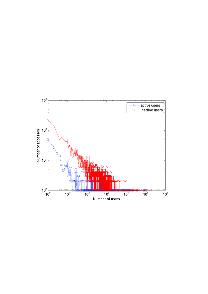
Figure 1: Log-log plot of wireless users’ activity

Our model is fully specified by the four input parameters $p,q,r$ and $k$, as described in Section 2. Of particular interest are the following probabilities:

1. $pr$, which is the rate at which new users join the network and attain their first wireless connection.

2. $p(1-r)$, which is the rate at which inactive users become active again.

3. $(1-p)q$, which is the rate at which active users attain a new wireless connection without first disconnecting from the network.

4. $(1-p)(1-q)$, which is that rate at which active users become inactive.

5. $k$, which can be viewed as the life of the network, assuming that the evolution takes place in discrete time steps, where at each time a single change occurs in the network according to the urn transfer model described in Section 2.

We processed the Dartmouth data set so that it contains pairs of users and their activity, where each user is identified by a client card and an activity corresponds to (1), (2), (3) or (4) above. We then estimated the probabilities $p,r$ and $q$ from the data, taking $k$ to be the number of pairs processed. From this we obtained, $p=0.0994$, $r=0.0046$, $q=0.8897$ and $k=13559701$.

Next we estimated $\varrho$ from (30) and $\tau$ from (31), obtaining $\varrho=0.1244$ and $\tau=6.9704$. Using (24) and (25) we estimated the exponent of the asymptotic power-law distribution as

$$\frac{\varrho+(1-q)\tau}{q}+1=2.0040.$$

As a validation of the model we populated the unstarred and starred urns according to the activity pairs from the processes data set. Then, using the methodology described in Section 4, we numerically minimised the least squares of the sum over $i$ of the differences between the number of balls in $urn_{i}$, respectively $urn^{*}_{i}$, and the predicted number of balls according to (23), and respectively (26), in accordance to (32). The fitted parameters we obtained from the unstarred urns using (23), were: $q=0.8901$, $\varrho=0.1101$ and $\tau=6.9648$, obtaining $(\varrho+(1-q)\tau)/q+1=1.9836$. The corresponding set of fitted parameters obtained from the starred urns using (26), were: $q=0.8898$, $\varrho=0.1385$ and $\tau=6.9473$, obtaining $(\varrho+(1-q)\tau)/q+1=2.0161$. As can be seen the fitted parameters are consistent with the ones we have mined from the original data set.

As a further validation of the model we ran a simulation implemented in Matlab according to the description of the stochastic process in Section 2, with the parameters $k=13559701$, $p=0.0994$, $r=0.0046$ and $q=0.8897$ as mined from the data set. We note that

$$p=0.0994>(1-p)(1-q)=0.0993$$

and

$$(1-p)(1-q)=0.0993>p(1-r)=0.0989$$

as required in the specification of the stochastic process in Section 2. So, for the probability of termination, with either all starred or unstarred urns being empty, to be less than $0.1$ we should set the initial number of balls in $urn_{1}$ to be $\delta=3600$, and the initial number of balls in $urn^{*}_{1}$ to be $\delta^{*}=600$. We verified this by running a simplified version of the simulation, which only accounts for the total number of balls in starred and unstarred urns. Out of ten simplified simulation runs with the above input parameters none terminated with all the unstarred or starred urns being empty.

We decided in our simulation to ignore the problem of empty urns, the justification being that having empty urns at some stage of the stochastic process does not have much effect on the exponent of the asymptotic power-law distribution, since by (30) and (31) the exponent given in (24) is approximately proportional to $pins_{k}+pins^{*}_{k}$, and by (28) the total number of pins depends only on the input parameters through independent random variables.

From $pins_{k}$ and $pins^{*}_{k}$ output from the simulation we computed $\varrho=0.1054$ from (30), $\tau=7.1442$ from (31), and finally the exponent of the asymptotic power-law distribution was computed as $(\varrho+(1-q)\tau)/q+1=2.0042$. As can be seen, the output from the simulation is consistent with the parameters mined from the data; a second simulation with the same input parameters produced similar results.

Overall, on the evidence from the computational results , the urn transfer model described in Section 2, is a viable model for a real social network, specifically for the access patterns of users within the Dartmouth wireless network.

6 Concluding Remarks

We have presented an extension of Simon’s classical stochastic process where each actor can be either in an active or an inactive state. Actors, chosen by preferential attachment may attain a new relation, become inactive or later become active again. The system is closed in the sense that once an actor enters the system he remains within the system. We have shown in (24) and (26) that, asymptotically, the number of active and inactive actors having prescribed number of relations is a power-law distribution. As a proof of concept we validated the model on a real data set of wireless accesses over a lengthy period of time. The validation made use of numerical optimisation rather than using standard regression tools, due to the known difficulty of detecting asymptotic power-law distributions in data.

The stochastic model we have presented is relevant to social networks where users may be active or inactive at different times. Two such real-world networks are wireless networks and peer-to-peer networks, although it remains to validate our model on a real peer-to-peer data set. In fact, our model could also be used to model user activity in an e-commerce portal or an online forum, where registration is required.

References

- [AB02] R. Albert and A.-L. Barabási. Statistical mechanics of complex networks. Reviews of Modern Physics, 74:47–97, 2002.
- [AS72] M. Abramowitz and I.A. Stegun, editors. Handbook of Mathematical Functions with Formulas, Graphs and Mathematical Tables. Dover, New York, NY, 1972.
- [ASBS00] L.A.N. Amaral, A. Scala, M. Barthélémy, and H.E. Stanley. Classes of small-world networks. Proceedings of the National Academy of Sciences of the United States of America, 97:11149–11152, 2000.
- [BKM+00] A. Broder, R. Kumar, F. Maghoul, P. Raghavan, A. Rajagopalan, R. Stata, A. Tomkins, and J. Wiener. Graph structure in the Web. Computer Networks, 33:309–320, 2000.
- [EMB02] H. Ebel, L.-I. Mielsch, and S. Bornholdt. Scale-free topology of e-mail networks. Physical Review E, 66:035103–1–035103–4, 2002.
- [FLL05] T.I. Fenner, M. Levene, and G. Loizou. A stochastic evolutionary model exhibiting power-law behaviour with an exponential cutoff. Physica A, 335:641–656, 2005.
- [FLL06] T.I. Fenner, M. Levene, and G. Loizou. A model for collaboration networks giving rise to a power law distribution with an exponential cutoff. Physics and Society Archive, physics/0503184, 2006. To appear in Social Networks.
- [GDJ06] S. Guha, N. Daswani, and R. Jain. An experimental study of the Skype peer-to-peer VoIP system. In Proceedings of International Workshop on Peer-to-Peer Systems (IPTPS), Santa Barbara, Ca., 2006.
- [GMY04] M.L. Goldstein, S.A. Morris, and G.G. Yen. Problem with fitting to the power-law distribution. European Physical Journal B, 41:255–258, 2004.
- [Gro02] J.W. Grossman. Patterns of collaboration in mathematical research. SIAM News, 35(9), 2002.
- [KE05] D. Kotz and K. Essien. Analysis of a campus wide wireless network. Wireless Networks, 11:115–133, 2005.
- [KH05] D. Kotz and T. Henderson. CRAWDAD: A community resource for archiving wireless data. IEEE Pervasive Computing, 4:12–14, 2005.
- [LFLW02] M. Levene, T.I. Fenner, G. Loizou, and R. Wheeldon. A stochastic model for the evolution of the Web. Computer Networks, 39:277–287, 2002.
- [LKR06] J. Liang, R. Kumar, and K.W. Ross. The FastTrack overlay: A measurement study. Computer Networks, 60:842–858, 2006.
- [New03] M.E.J. Newman. The structure and function of complex networks. SIAM Review, 45:167–256, 2003.
- [Ora01] A. Oram. Peer-to-Peer: Harnessing the Power of Disruptive Technologies. O’Reilly, Sebastopol, Ca., 2001.
- [PGES05] J.A. Pouwelse, P. Garbacki, D.H.J. Epema, and H.J. Sips. The Bittorrent p2p file-sharing system: Measurements and analysis. In Proceedings of International Workshop on Peer-to-Peer Systems (IPTPS), Ithaca, NY, 2005.
- [Pri76] D.J. de Solla Price. A general theory of bibliometric and other cumulative advantage processes. Journal of the American Society of Information Science, 27:292–306, 1976.
- [RIF02] M. Ripeanu, A. Iamnitchi, and I. Foster. Mapping the Gnutella network. IEEE Internet Computing, 6:50–57, 2002.
- [Ros83] S.M. Ross. Introduction to Stochastic Dynamic Programming. Academic Press, New York, NY, 1983.
- [Sch91] M. Schroeder. Fractals, Chaos, Power Laws: Minutes from an Infinite Paradise. W.H. Freeman, New York, NY, 1991.
- [Sco00] J. Scott. Social Network Analysis. Sage Publications, London, 2nd edition, 2000.
- [Sim55] H.A. Simon. On a class of skew distribution functions. Biometrika, 42:425–440, 1955.