Bayesian Analysis of the Conditional Correlation Between Stock Index Returns with Multivariate SV Models

Abstract

In the paper we compare the modelling ability of discrete-time multivariate Stochastic Volatility models to describe the conditional correlations between stock index returns. We consider four trivariate SV models, which differ in the structure of the conditional covariance matrix. Specifications with zero, constant and time-varying conditional correlations are taken into account. As an example we study trivariate volatility models for the daily log returns on the WIG, S&P $500$, and FTSE $100$ indexes. In order to formally compare the relative explanatory power of SV specifications we use the Bayesian principles of comparing statistic models. Our results are based on the Bayes factors and implemented through Markov Chain Monte Carlo techniques. The results indicate that the most adequate specifications are those that allow for time-varying conditional correlations and that have as many latent processes as there are conditional variances and covariances. The empirical results clearly show that the data strongly reject the assumption of constant conditional correlations.

89.65 Gh, 05.10 Gg

1 Introduction

There are a lot of theoretical and empirical reasons to study multivariate volatility models. Analysis of financial market volatility and correlations among markets play a crucial role in financial decision making (e.g. hedging strategies, portfolio allocations, Value-at-Risk calculations). The correlations among markets are very important in the global portfolio diversification.
The main aim of the paper is to compare the modelling ability of discrete-time Multivariate Stochastic Volatility (MSV) models to describe the conditional correlations and volatilities of stock index returns. The MSV models offer powerful alternatives to multivariate GARCH models in accounting for properties of the conditional variances and correlations. Superior performance of bivariate SV models over GARCH models (in term of the Bayes factor) are documented in [8]. But the MSV models are not as often used in empirical applications as the GARCH models. The main reason is that the SV models are more difficult to estimate. In this paper we consider four multivariate Stochastic Volatility models, including the specification with zero, constant and time-varying conditional correlations. These MSV specifications are used to model volatilities and conditional correlations between stock index returns. We study trivariate volatility models for the daily log returns on the WIG index, the Standard & Poor’s $500$ index, and the FTSE $100$ index for the period January $4$, $1999$ to December $30$, $2005$. In the next section the Bayesian statistical methodology is briefly presented . In section $3$ the model framework is introduced. Section $4$ is devoted to the description of trivariate SV specifications. In section $5$ we present and discuss the empirical results.

2 Bayesian statistical methodology

Let $\mathbf{y}$ be the observation matrix and $\theta_{i}$ be the vector of unknown parameters and $\omega_{i}$ the latent variable vector in model $M_{i}$ $(i=1,2,\ldots,n)$. The $i$ - the Bayesian model is characterized by the joint probability density function, which can be written as the product of three densities:

$$p(\mathbf{y},\omega_{i},\theta_{i}|y_{(0)},M_{i})=p(\mathbf{y}|\omega_{i},\theta_{i},y_{(0)},M_{i})p(\omega_{i}|\theta_{i},M_{i})p(\theta_{i}|M_{i}),\;i=1,2,\ldots,n,$$

where $y_{(0)}$ denotes initial conditions, $p(\mathbf{y}|\omega_{i},\theta_{i},y_{(0)},M_{i})$ is the conditional density of $\mathbf{y}$ when $\omega_{i}\in\Omega_{i},\theta_{i}\in\Theta_{i}$ are given, $p(\omega_{i}|\theta_{i},M_{i})$ is the density of the latent variables conditioned on $\theta_{i}$, $p(\theta_{i}|M_{i})$ is the prior density function under $M_{i}$. The joint probability density function can be expressed as the product of the marginal data density of the observation matrix (given the initial conditions $y_{(0)}$) in model $M_{i}$: $p(\mathbf{y}|y_{(0)},M_{i})$, and the posterior density function of the parameter vector $\theta_{i}$ and the latent variable vector $\omega_{i}$ in $M_{i}$: $p(\omega_{i},\theta_{i}|\mathbf{y},y_{(0)},M_{i})$, i.e.

$$p(\mathbf{y},\omega_{i},\theta_{i}|y_{(0)},M_{i})=p(\omega_{i},\theta_{i}|\mathbf{y},y_{(0)},M_{i})p(\mathbf{y}|y_{(0)},M_{i}),$$

where

$$p(\mathbf{y}|y_{(0)},M_{i})=\int_{\Omega_{i}\times\Theta_{i}}p(\mathbf{y}|\omega_{i},\theta_{i},y_{(0)},M_{i})p(\omega_{i},\theta_{i}|M_{i})d\omega_{i}d\theta_{i}.$$

The statistical inference is based on the posterior distributions, while the marginal densities $p(\mathbf{y}|y_{(0)},M_{i})$ $(i=1,2,\ldots,n)$ are the crucial components in model comparison.
Assume that $M_{1},\ldots,M_{n}$ are mutually exclusive (non-nested) and jointly exhaustive models. From Bayes’s theorem, it is easy to show that the posterior probability of $M_{i}$ is given by:

$$p(M_{i}|\mathbf{y},y_{(0)})=\frac{p(M_{i})p(\mathbf{y}|y_{(0)},M_{i})}{\sum_{i=1}^{n}p(M_{i})p(\mathbf{y}|y_{(0)},M_{i})},$$

where $p(M_{i})$ denotes the prior probability of $M_{i}$. For the sake of pairwise comparison, we use the posterior odds ratio, which for any two models $M_{i}$ and $M_{j}$ is equal to the prior odds ratio times the ratio of the marginal data densities:

$$\frac{p(M_{i}|\mathbf{y},y_{(0)})}{p(M_{j}|\mathbf{y},y_{(0)})}=\frac{p(M_{i})}{p(M_{j})}\cdot\frac{p(\mathbf{y}|y_{(0)},M_{i})}{p(\mathbf{y}|y_{(0)},M_{j})}.$$

The ratio of the marginal data densities is called the Bayes factor:

$$B_{ij}=\frac{p(\mathbf{y}|y_{(0)},M_{i})}{p(\mathbf{y}|y_{(0)},M_{j})}.$$

Thus, assuming equal prior model probabilities (i.e. $p(M_{i})=p(M_{j})$), the Bayes factor is equal to the posterior odds ratio. We see that the values of the marginal data densities for each model are the main quantities for Bayesian model comparison. The marginal data density in model $M_{i}$ can be written as:

$$p(\mathbf{y}|y_{(0)},M_{i})=\left(\int_{\Omega_{i}\times\Theta_{i}}\left[p(\mathbf{y}|\omega_{i},\theta_{i},y_{(0)},M_{i})\right]^{-1}p(\omega_{i},\theta_{i}|\mathbf{y},y_{(0)},M_{i})d\omega_{i}d\theta_{i}\right)^{-1}$$

Of course, in the case of SV models this integral can not be evaluated analytically and thus must be computed by numerical methods. We use the method proposed by [6], which approximates the marginal data density by the harmonic mean of the values $p(\mathbf{y}|\omega_{i},\theta_{i},y_{(0)},M_{i})$, calculated for the observed matrix $\mathbf{y}$ and for the vector $(\omega_{i}^{(q)},\theta_{i}^{(q)})^{\prime}$ drawn from the posterior distribution. That is:

$$\hat{p}(\mathbf{y}|y_{(0)},M_{i})=\left(\frac{1}{m}\sum_{q=1}^{m}\frac{1}{p(\mathbf{y}|\omega_{i}^{(q)},\theta_{i}^{(q)},y_{(0)},M_{i})}\right)^{-1}.$$

The estimator $\hat{p}(\mathbf{y}|y_{(0)},M_{i})$ is very easy to calculate and gives results that are precise enough for our model comparison.

3 Model framework

Let $x_{jt}$ denote the price of asset $j$ (or index quotations as in our application) at time $t$ for $j=1,2,3$ and $t=1,2,\ldots,T$. The vector of growth rates $y_{t}=(y_{1,t},y_{2,t},y_{3,t})^{\prime}$, each defined by the formula $y_{j,t}=100\ln\left(x_{t,j}/x_{j,t-1}\right)$, is modelled using the VAR(1) framework:

$$y_{t}-\delta=R(y_{t-1}-\delta)+\xi_{t},\;\;\;t=1,2,\ldots,T,$$

where $\{\xi_{t}\}$ is a trivariate SV process, $T$ denotes the number of the observations used in estimation. More specifically:

$$\left[\begin{array}[]{c}y_{1,t}\\ y_{2,t}\\ y_{3,t}\\ \end{array}\right]-\left[\begin{array}[]{c}\delta_{1}\\ \delta_{2}\\ \delta_{3}\\ \end{array}\right]=\left[\begin{array}[]{ccc}r_{11}&r_{12}&r_{13}\\ r_{21}&r_{22}&r_{23}\\ r_{31}&r_{32}&r_{33}\\ \end{array}\right]\left(\left[\begin{array}[]{c}y_{1,t-1}\\ y_{2,t-1}\\ y_{3,t-1}\\ \end{array}\right]-\left[\begin{array}[]{c}\delta_{1}\\ \delta_{2}\\ \delta_{3}\\ \end{array}\right]\right)+\left[\begin{array}[]{c}\xi_{1,t}\\ \xi_{2,t}\\ \xi_{3,t}\\ \end{array}\right].$$

We assume that, conditionally on the latent variable vector $\Omega_{t(i)}$ and on the parameter vector $\theta_{i},\xi_{t}$ follows a trivariate Gaussian distribution with mean vector $0_{[3\times 1]}$ and covariance matrix $\Sigma_{t}$, i.e.

$$\xi_{t}|\Omega_{t(i)},\theta_{i}\sim N(0_{[3\times 1]},\Sigma_{t}),\;\;t=1,2,\dots,T.$$

Competing trivariate SV models are defined by imposing different structures on $\Sigma_{t}$.
For all elements of $\delta$ and $R$ we assume the multivariate standardized Normal prior $N(0,I_{15})$, truncated by the restriction that all eigenvalues of $R$ lie inside the unit circle. We assume that the matrix $[\delta,R]$ and the remaining (model-specific) parameters are prior independent.

4 Trivariate VAR(1) - SV models

4.1 Stochastic Discount Factor Model (SDF)

The first specification considered here is the stochastic discount factor model (SDF) proposed, but not applied, by [4]. The SDF process is defined as follows:

$$\begin{array}[]{rcl}\xi_{t}=\varepsilon_{t}\sqrt{h_{t}},&&\varepsilon_{t}\sim iiN(0_{[3\times 1]},\Sigma),\\ \ln h_{t}=\phi\ln h_{t-1}+\sigma_{h}\eta_{t},&&\eta_{t}\sim iiN(0,1),\\ \varepsilon_{j,t}\perp\eta_{s},&&t,s\in\mathbf{Z},\;j=1,2,3,\end{array}$$

where $\mathbf{Z}=\{\dots,-2,-1,0,1,2,\ldots\}$, $\perp$ denotes independence, and the symbol $\eta_{t}\sim iiN(0,1)$ denotes a series of independently and normally distributed random variables with mean vector $0_{[3\times 1]}$ and covariance matrix $\Sigma$. In this case, we have

$$\xi_{t}|\Omega_{t(1)},\Sigma\sim(0_{[3\times 1]},h_{t}\Sigma),$$

where $\Omega_{t(1)}=h_{t}$. The conditional covariance matrix of $\xi_{t}$ is time varying and stochastic, but all its elements have the same dynamics governed by $h_{t}$. Consequently, the conditional correlation coefficients are constant over time. Our model specification is completed by assuming the following prior structure:

$$p(\phi,\sigma_{h}^{2},\ln h_{0},\Sigma)=p(\phi)p(\sigma_{h}^{2})p(\ln h_{0})p(\Sigma),$$

where we use proper prior densities of the following distributions:
$\phi\sim N(0,100)I_{(-1,1)}(\phi),\;\;\sigma_{h}^{2}\sim IG(1,0.005),\;\;\ln h_{0}\sim N(0,100),\;\\ \Sigma\sim IW(3I,3,3)$.
The symbol $N(a,b)$ denotes the normal distribution with mean $a$ and variance $b$, $I_{(-1,1)}(.)$ is the indicator function of the interval $(-1,1)$. $IG(\nu_{0},s_{0})$ denotes the inverse Gamma distribution with mean $s_{0}/(\nu_{0}-1)$ and variance $s_{0}^{2}/[(\nu_{0}-1)^{2}(\nu_{0}-2)]$. The symbol $IW(B,d,3)$ denotes the three-dimensional inverse Wishart distribution with $d$ degrees of freedom and parameter matrix $B$. The initial condition for $\ln h_{t}$ (i.e. $\ln h_{0}$) is treated as an additional parameter and estimated jointly with other parameters.

4.2 Basic Stochastic Volatility Model (BSV)

Next, we consider the basic stochastic volatility process (BSV), where $\xi_{t}|\Omega_{t(2)}\sim N(0_{[3\times 1]},\Sigma_{t}),$ and $\Sigma_{t}=Diag(h_{1,t},h_{2,t},h_{3,t})$ (similar to the idea of [2]). The conditional variance equations are:

$$\ln h_{j,t}-\gamma_{jj}=\phi_{jj}(\ln h_{j,t-1}-\gamma_{jj})+\sigma_{jj}\eta_{j,t},$$

for $j=1,2,3$, where $\eta_{t}\sim iiN(0_{[3\times 1]},I_{3})$, $\eta_{t}=(\eta_{1,t},\eta_{2,t},\eta_{3,t})^{\prime}$, $\Omega_{t(2)}=(h_{1,t},h_{2,t},h_{3,t})^{\prime}$. For the parameters we use the same specification of prior distribution as in the univariate SV model (see [9]), i.e. $(\gamma_{jj},\phi_{jj})^{\prime}\sim N(0,100I)I_{(-1,1)}(\phi_{jj}),\;\;\sigma_{h}^{2}\sim IG(1,0.005),\;\;\ln h_{j,0}\sim N(0,100),\;\;j=1,2,3.$

4.3 JSV Model

Both previous specifications (SDF and BSV) are very restrictive. Now, we propose a SV process based on the spectral decomposition of the matrix $\Sigma_{t}$. That is

$$\Sigma_{t}=P\Lambda_{t}P^{-1},$$

where $\Lambda_{t}$ is the diagonal matrix consisting of all eigenvalues of $\Sigma_{t}$, and $P$ is the matrix consisting of the eigenvectors of $\Sigma_{t}$. For series $\{\ln\lambda_{j,t}\}$ $(j=1,2,3)$, similarly as in the univariate SV process, we assume standard univariate autoregressive processes of order one, namely

$$\ln\lambda_{j,t}-\gamma_{jj}=\phi_{jj}(\ln\lambda_{j,t-1}-\gamma_{jj})+\sigma_{jj}\eta_{j,t},$$

for $j=1,2,3$ , where $\eta_{t}\sim iiN(0_{[3\times 1]},I_{3})$, $\eta_{t}=(\eta_{1,t},\eta_{2,t},\eta_{3,t})^{\prime}$, and $\Omega_{t(3)}=(\lambda_{1,t},\lambda_{2,t},\lambda_{3,t})^{\prime}$. This reparametrization of $\Sigma_{t}$ does not require any parameter constraints to ensure positive definiteness of $\Sigma_{t}$. If $|\phi_{jj}|<1\;\;(j=1,2,3)$ then $\{\ln\lambda_{1,t}\}$, $\{\ln\lambda_{21,t}\}$ and $\{\ln\lambda_{3,t}\}$ are stationary and the JSV process is a white noise. In addition, $P$ is an orthogonal matrix, i.e. $P^{\prime}P=I_{2}$, thus $P$ is parametrized by three parameters (Euler angles) $\kappa_{j}\in(-\pi,\pi)$, $j\in\{1,2,3\}$:

$$P(\kappa_{1},\kappa_{2},\kappa_{3})=P_{1}(\kappa_{1})P_{2}(\kappa_{2})P_{3}(\kappa_{3}),$$

where for $l=1,3$

$$P_{l}(\kappa_{l})=\left[\begin{array}[]{ccc}\cos\kappa_{l}&-\sin\kappa_{l}&0\\ \sin\kappa_{l}&\cos\kappa_{l}&0\\ 0&0&1\end{array}\right],\quad P_{2}(\kappa_{2})=\left[\begin{array}[]{ccc}1&0&0\\ 0&\cos\kappa_{2}&-\sin\kappa_{2}\\ 0&\sin\kappa_{2}&\cos\kappa_{2}\end{array}\right].$$

In this case the conditional correlation coefficients are time-varying and stochastic if $\kappa_{j}\neq 0$ for some $j\in\{1,2,3\}$. For the model-specific parameters we take the following prior distributions: $(\gamma_{jj},\phi_{jj})^{\prime}\sim N(0,100I)I_{(-1,1)}(\phi_{jj}),\;\\ \sigma_{jj}^{2}\sim IG(1,0.005),\;\;\ln\lambda_{j,0}\sim N(0,100)$, $\kappa_{j}\sim U(-\pi,\pi)$ (i.e. uniform over $(-\pi,\pi)$), $j=1,2,3$. The BSV model can be obtained by imposing the parameter restrictions $\kappa_{1}=\kappa_{2}=\kappa_{3}=0$ in the $P$ definition of the JSV model (but we formally exclude this value).

4.4 TSV Model

The next specification (proposed by [13], thus called TSV) uses six separate latent processes (the number of the latent processes is now equal to the number of distinct elements of the conditional covariance matrix). Following the definition in [13], we propose to use the Cholesky decomposition:

$$\Sigma_{t}=L_{t}G_{t}L_{t}^{\prime},$$

where $L_{t}$ is a lower triangular matrix with unitary diagonal elements, $G_{t}$ is a diagonal matrix with positive diagonal elements:

$$L_{t}=\left[\begin{array}[]{ccc}1&0&0\\ q_{21,t}&1&0\\ q_{31,t}&q_{32,t}&1\\ \end{array}\right],\quad G_{t}=\left[\begin{array}[]{ccc}q_{11,t}&0&0\\ 0&q_{22,t}&0\\ 0&0&q_{33,t}\\ \end{array}\right],$$

that is

$$\Sigma_{t}=\left[\begin{array}[]{ccc}q_{11,t}&q_{11,t}q_{21,t}&q_{11,t}q_{31,t}\\ q_{21,t}q_{11,t}&q_{11,t}q_{21,t}^{2}+q_{22,t}&q_{11,t}q_{21,t}q_{31,t}+q_{22,t}q_{32,t}\\ q_{31,t}q_{11,t}&q_{11,t}q_{21,t}q_{31,t}+q_{22,t}q_{32,t}&q_{11,t}q_{31,t}^{2}+q_{22,t}q_{32,t}^{2}+q_{33,t}\\ \end{array}\right].$$

Series $\{q_{ij,t}\}$, and $\{\ln q_{jj,t}\}$ $(i,j=1,2,3,\quad i>j)$, analogous to the univariate SV, are standard univariate autoregressive processes of order one, namely

$$\ln q_{jj,t}-\gamma_{jj}=\phi_{jj}(\ln q_{jj,t-1}-\gamma_{jj})+\sigma_{jj}\eta_{jj,t},\;\;\>j=1,2,3,$$

$$q_{ij,t}-\gamma_{ij}=\phi_{ij}(q_{ij,t-1}-\gamma_{ij})+\sigma_{ij}\eta_{ij,t},\quad j,i\in\{1,2,3\},\quad i>j,$$

$$\eta_{t}=(\eta_{11,t},\eta_{22,t},\eta_{33,t},\eta_{21,t},\eta_{31,t},\eta_{32,t})^{\prime}\sim iiN_{6}(0_{[6\times 1]},I_{6}),\quad t\in\mathbf{Z},$$

$$\Omega_{t(4)}=(q_{11,t},q_{22,t},q_{33,t},q_{21,t},q_{31,t},q_{32,t})^{\prime}.$$

Note that positive definiteness of $\Sigma_{t}$ is achieved by modelling $\ln q_{jj,t}$ instead of $q_{jj,t}$ . It is easy to show that if the absolute values of $\phi_{ij}$ are less than one the TSV process is a white noise (see [10]). We see that the TSV model is able to model both the time-varying conditional correlation coefficients and variances of returns. A major drawback of this process is that the conditional variances and covariances are not modelled in a symmetric way, thus the explanatory power of model may depend on the ordering of financial instruments.
We assume the following prior distributions:
$(\gamma_{ij},\phi_{ij})^{\prime}\sim N(0,100I)I_{(-1,1)}(\phi_{ij})$, $\sigma_{ij}^{2}\sim IG(1,0.005)$, $\ln q_{ii,0}\sim N(0,100)$ for $i,j\in\{1,2,3\}$ and $i\geq j$ ; $q_{ij,0}\sim N(0,100)$ for $i,j\in\{1,2,3\}$, $i>j$. The prior distributions used are relatively noninformative. Note that the BSV model can be obtained as a limiting case, corresponding to $\gamma_{ij}=\phi_{ij}=0,$ $\sigma_{ij}^{2}\to 0$ for $i,j\in\{1,2,3\}$, $i>j$.

5 Empirical results

We consider daily stock index returns for three national markets: Poland (WIG), the United States (S&P $500$), and the United Kingdom (FTSE $100$), from January $4,1999$ to December $30,2005$. We consider only index closing quotations in trading days for all considered national markets, thus our sample consists of $1701$ daily observations . The first observation is used to construct initial conditions. Thus T, the length of the modelled vector time series, is equal to $1700$.

Table 1: Logs of Bayes factors in favour of $TSV_{FSW}$ model

Model	Number of latent	Number of	$\log_{10}(B_{4,1,i})$	Rank
	processes	parameters
$M_{4,1}$ $(TSV_{FSW})$	6	12+24	0.00	1
$M_{4,2}$ $(TSV_{FWS})$	6	12+24	7.82	2
$M_{4,3}$ $(TSV_{SWF})$	6	12+24	15.55	3
$M_{4,4}$ $(TSV_{SFW})$	6	12+24	15.86	4
$M_{4,5}$ $(TSV_{WFS})$	6	12+24	17.05	5
$M_{4,6}$ $(TSV_{WSF})$	6	12+24	22.96	6
$M_{3}$ (JSV)	3	12+15	63.68	7
$M_{1}$ (SDF)	1	12+9	87.39	8
$M_{2}$ (BSV)	3	12+12	181.18	9

In Table 1 we present the decimal logarithms of the Bayes factors in favor of $TSV_{FSW}$ model. Our posterior results are obtained using MCMC methods: Metropolis-Hastings within the Gibbs sampler (see [11], [7] and [3]). The results presented in this paper are based on $500,000$ states of the Markov chain, generated after $100,000$ burnt-in states. The Bayes factors are calculated using the Newton and Raftery’s method [6]. Because in the TSV specification the conditional variances are not modelled in a symmetric way, we consider six cases: $TSV_{FSW}$, $TSV_{FWS}$, $TSV_{SWF}$, $TSV_{SFW}$, $TSV_{WFS}$, and $TSV_{WSF}$. These models differ in ordering of elements in $y_{t}$. For example in the $TSV_{FSW}$ model $y_{1,t}$ denotes the daily growth rate of the FTSE $100$ index at day $t$, and $y_{2,t}$ and $y_{3,t}$ are respectively the daily growth rates of the S&P $500$ and the WIG indexes at day $t$.
Our findings show clear superiority of the TSV specifications (which describe the six distinct elements of the conditional covariance matrix by six separate latent processes) over all SV models considered here. The $TSV_{FSW}$ model receives almost all posterior probability mass (assuming equal prior model probabilities), being about $7.82$ orders of magnitude more probable a posterior than the $TSV_{FWS}$ model and $63.68$ orders of magnitude better than the JSV model. Furthermore, the $TSV_{WSF}$ model fits the data about $23$ orders of magnitude worse than the best TSV model. It is mainly attributed to the fact that the growth rates of the FTSE index are less volatile than the S&P and WIG indexes. When we compare the unconditional variance of $\xi_{j,t}$ $(Var(\xi_{j,t})=\exp\left(\gamma_{jj}+0.5\sigma_{jj}^{2}/(1-\phi_{jj}^{2})\right),\;\;j=1,2,3)$ obtained in the BSV model, we observe a value of $1.448$ for the WIG index, $0.955$ for the S&P $500$ index and $0.943$ for the FTSE index. It is in accordance with the ordering of returns in the best TSV model. Thus, the explanatory power of the SV model depends not only on the number of latent processes, but also on the ordering of financial instruments in case of the TSV specifications. The results indicate that the return rates of the WIG, S&P and FTSE indexes reject the constant or zero conditional correlation hypothesis, represented by the SDF and BSV model.
The main characteristics of the posterior distributions of the conditional correlation coefficients are presented in Figure 1, where the upper line represents the posterior mean plus standard deviation the lower one - the posterior mean minus standard deviation. The conditional correlation coefficients produced by our VAR(1)-SV models with at least three latent processes vary markedly over time. Surprisingly, the TSV models with different ordering of the returns lead to different posterior inference on the conditional covariances. The differences in the dynamics of conditional correlations are understandable because of the structure of the conditional covariance matrix. In the TSV models the conditional covariance between $\xi_{1,t}$ and $\xi_{2,t}$ (similarly between $\xi_{1,t}$ and $\xi_{3,t}$) depends on the variance of $\xi_{1,t}$ (i.e. $q_{11,t}$). Thus, a large increase in the conditional variance of $\xi_{1,t}$ leads to an increase in the conditional covariance. Therefore the $TSV_{WSF}$ and $TSV_{WFS}$ models (in which the WIG index is the first component) lead to similar inference on the dynamics of the conditional correlations. The plots of the posterior means of $\rho_{ij,t}$, obtained in the remaining TSV models are different (because of differences in volatilities of the S&P$500$, FTSE indexes and WIG index). Note also that in the JSV model the latent processes that describe volatilities are included in the conditional correlation coefficient definitions. Consequently, the conditional correlations depend on the volatilities. Surprisingly, in the SDF model the conditional correlations are estimated very precisely - the posterior standard deviations of $\rho_{ij,t}$ are relatively small. The returns on the WIG index are lower correlated with returns on the S&P $500$ index (with an average of $0.18$) than with returns on the FTSE index (with an average of $0.24$). This low correlation is partially explained by the non - overlapping trading hours of U.S. market with the European markets. The U.S. market (represented by the S&P $500$ index) has the average correlation of $0.47$ with the U.K. market. Finally, it is important to stress that our results show that the conditional correlations are not significantly higher when world markets are down trending, which is in contrast to the results presented in the papers: [1], [12], [5].

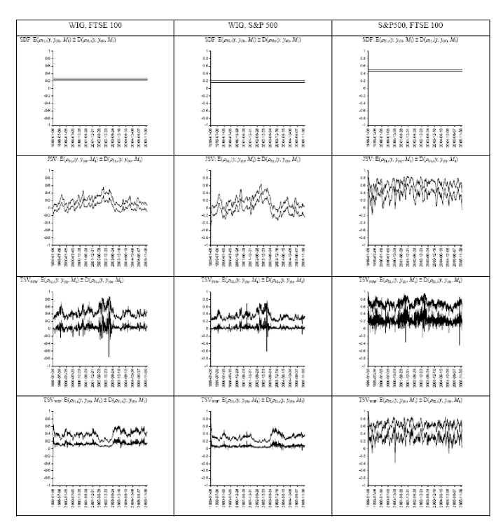
Figure 1: Conditional correlation coefficients (posterior mean $\pm 1$ standard deviation)

References

• [1] Ang A., Bekaert G. (2002), International Asset Allocation With Regime Shifts, The Review of Financial Studies 15, 1137-1187
• [2] Harvey A. C., Ruiz E., Shephard N.G. (1994), Multivariate Stochastic Variance Model, Review of Economic Studies, vol.61
• [3] Gamerman D. (1997), Markov Chain Monte Carlo. Stochastic Simulation for Bayesian Inference, Champan and Hall, London
• [4] Jacquier E., Polson N., Rossi P., (1995), Model and Prior for Multivariate Stochastic Volatility Models, technical report, University of Chicago, Graduate School of Business
• [5] Longin F., Solnik B., (2001), Extreme Correlation of International Equity Markets, The Journal of Finance, vol. 56, no. 2, 649-676
• [6] Newton M.A., Raftery A.E., (1994), Approximate Bayesian inference by the weighted likelihood bootstrap (with discussion), Journal of the Royal Statistical Society B, vol. 56, No. 1
• [7] O’Hagan A. (1994) Bayesian Inference, Edward Arnold, London
• [8] Osiewalski J., Pajor A., Pipie M. (2006) Bayes factors for bivariate GARCH and SV models, Acta Universitatis Lodziensis - Folia Oeconomica, forthcoming
• [9] Pajor A., (2003), Procesy zmienno ci stochastycznej w bayesowskiej analizie finansowych szereg w czasowych (Stochastic Volatility Processes in Bayesian Analysis of Financial Time Series), doctoral dissertation (in Polish), published by Cracow University of Economics, Krak w
• [10] Pajor A., (2005a), Bayesian Analysis of Stochastic Volatility Model and Portfolio Allocation, [in:] Issues in Modelling, Forecasting and Decision-Making in Financial Markets, Acta Universitatis Lodzensis - Folia Oeconomica 192, 229-249
• [11] Pajor A. (2006), VECM-TSV Models for Exchange Rates of the Polish Zloty, [in:] Issues in Modelling, Forecasting and Decision-Making in Financial Markets, Acta Universitatis Lodzensis - Folia Oeconomica, forthcoming
• [12] Solnik B, Boucrelle C., Fur L. Y., (1996), International Market Correlation and Volatility, Financial Analysis Journal vol.52, no.5, 17-34
• [13] Tsay R.S., (2002), Analysis of Financial Time Series. Financial Econometrics, A Wiley-Interscience Publication, John Wiley & Sons, INC
Refer to caption