GLD Detector Outline Document Version 1.2

Postal address to contact:
¹ Academia Sinica, P. O. Box 2735, Beijing 100080, China
² Akita Keizaihoka University, 46-1, Morisawa, Shimokitadezakura, Akita 010-8515, Japan
³ Carleton University, 1125 Colonel By Drive, Ottawa, Ontanio, K1S 5B6, Canada
⁴ CEA, DAPNIA/SPP, CE-Saclay, 91191 Gif-sur-Yvette, France
⁵ Chonbuk National University, 664-14, 1ga Duckjin-Dong, Duckjin-Gu, Chonju, Chonbuk 561-756, Korea
⁶ Chonnam National University, 300 Yong-Bong, Kwangju 500-757, Korea
⁷ Cornell University, Ithaca, NY 14853-5001, USA
⁸ DESY, Notkestrasse 85, D-22603, Hamburg, Germany
⁹ Ewha Womans University, Daehyun-dong, Seodaemun-gu, Seoul 120-750, Korea
¹⁰ Hiroshima University, 1-3-1 Kagamiyama, Higashi-Hiroshima 739-8526, Japan
¹¹ Ibaraki College of Technology, 866 Nakane, Hitachinaka-shi, Ibaraki 312-8508, Japan
¹² IHEP, PO Box 918, Beijing 100039, China
¹³ Indian Institute of Science, Bangalore 560 012, India
¹⁴ INFN Sezione di Padova, Universita di Padova, I-35131 Padova, Italy
¹⁵ INFN, University of Pisa, I-56000 Pisa, Italy
¹⁶ Institute of Physics, PO. Box 429, Boho, Hanoi 10000, Vietnam
¹⁷ ITEP, B. Cheremushkinskaya ul. 25, RU-117259 Moscow, Russia
¹⁸ KAIST, 373-1 Kusong-dong, Yusong-ku, Daejon 305-701, Korea
¹⁹ KEK, 1-1 Oho, Tsukuba, Ibaraki 305-0801, Japan
²⁰ KIAS, 207-43 Cheongryangri-dong, Dongdaemun-gu, Seoul 130-012, Korea
²¹ Kinki University, 3-4-1, Kowakae, Higashi Osaka, Osaka 577-8502, Japan
²² Kobe University, 1-1 Rokkodai-cho, Nada-ku, Kobe 657, Japan
²³ Kogakuin University, 2665-1 Nakano, Hachioji, Tokyo 192-0015, Japan
²⁴ Konkuk University, Hwayang-dong, Kwangjin-gu, Seoul 143-701, Korea
²⁵ Korea University, Anam-dong, Sungbuk-gu, Seoul 136-701, Korea
²⁶ Konan University, 6-1-1, Nishiokamoto, Higashinadaku, Kobe 658-8501, Japan
²⁷ Kyoto University, Oiwake-cho, Kitashirakawa, Sakyo-ku, Kyoto 606-8224, Japan
²⁸ Kyungpook National University, Sankyuk-dong, Buk-gu, Daegu 702-701, Korea
²⁹ LBL, 1 Cyclotron Road, Berkeley, CA 94720, USA
³⁰ Max-Planck-Institut fuer Physik, Fohringer Ring 6, D-80805, Munchen, Germany
³¹ MECIT, P.B. No. 79, Al Rusayl, Postal Code: 124, Sultanate of Oman
³² Mindanao Polytechnic State College, Lapasan, Cagayan de Oro City 9000, Philippines
³³ Mindanao State University, Iligan Institute of Technology, 9200 Iligan city, Philippines
³⁴ Miyagi Gakuin, 9-1-1, Sakuragaoka, Aoba-ku, Sendai 981-8557, Japan
³⁵ Nagoya University, Furo-cho, Chikusa-ku, Nagoya 464-8601, Japan
³⁶ National Central University, Chung-Li 320, Taiwan
³⁷ NIRS, 4-9-1, Anagawa, Inage, Chiba, 263-8555 Japan
³⁸ National Taiwan University, Taipei 10617, Taiwan
³⁹ National University of Singapore, Block S12, Lower Kent Ridge Road 119260, Republic of Singapore
⁴⁰ Niigata University, Ikarashi 2-no-cho 8050, Niigata, Niigata 950-2181, Japan
⁴¹ Niihama NCT, 7-1, Yakumo-cho, Niihama, Ehime 792-8580, Japan
⁴² Nuclear Science Centre, Post Box 10502, New Delhi, 110067, India
⁴³ Ochanomizu University, 1 Ohtsuka 2-1, Bunkyo-ku, Tokyo 112-8610, Japan
⁴⁴ Osaka City University, 3-3-138 Sugimoto, Sumiyoshi-ku, Osaka 558-8585, Japan
⁴⁵ Osaka University, 1-1 Machikaneyama, Toyonaka, Osaka 560-0043, Japan
⁴⁶ Oxford University, Oxford OX1 3RH, United Kingdom
⁴⁷ Physical Institut, Bonn University, Nussallee 12, D-53115 Bonn, Germany
⁴⁸ Radboud University Nijmegen, PO Box 9102, 6500 HC Nijmegen, The Netherlands
⁴⁹ Rutherford Appleton Laboratory, Chilton, DIDCOT, Oxon, OX1110QX, United Kingdom
⁵⁰ Saga University, 1 Honjo-machi, Saga-shi 840-8502, Japan
⁵¹ Seoul National University, Shinlim-dong, Kwanak-gu, Seoul 151-742, Korea
⁵² Shandong University, Jinan, Shandong, 250100, China
⁵³ Shinshu University, 3-1-1, Asahi, Matsumoto, Nagano 390-8621, Japan
⁵⁴ SLAC, PO Box 4349, Stanford, CA 94309-4349, USA
⁵⁵ Sungkyunkwan University, Cheoncheon-dong, Jangan-gu, Suwon, Gyeonggi-do 440-746, Korea
⁵⁶ Graduate University for Advanced Studies, Shonan Village, Hayama, Kanagawa 240-0193, Japan
⁵⁷ The Institute of Mathematical Sciences, Taramani, Chennai 600 113, India
⁵⁸ Tata Institute of Fundamental Research, Homi Bhabha Road, Mumbai 400 005, India
⁵⁹ Tohoku University, Aoba, Aramaki, Aoba-ku, Sendai 980-8578, Japan
⁶⁰ Tohokugakuin University, 1-13-1, Chuo, Tagajo, Migagi 985-8537, Japan
⁶¹ Tokushima University, Tokushima 770-8502, Japan
⁶² Tokyo A&T, Nakacho 2-24-16, Koganeishi, Tokyo 184-8588, Japan
⁶³ Toyama NCMT, 1-2 Ebie Neriya, Shinminato, Toyama 933-0293, Japan
⁶⁴ Tsinghua University, Beijing 100084, China
⁶⁵ UC Santa Cruz, Santa Cruz, CA 95064, USA
⁶⁶ University College London, London, England WC1E 6BT
⁶⁷ University of Texas at Arlington, PO Box 19059, Arlington, TX 76019, USA
⁶⁸ University of Cambridge, Madingley Road, Cambridge CB3 0HE, UK
⁶⁹ University of Colorado, Campus Box 390, Boulder, CO 80309, USA
⁷⁰ University of Florida, Gainesville, Florida 33611, USA
⁷¹ University of Kansas, Manhattan, KS 66506-26031, USA
⁷² University of Melbourne, Parkville, Victoria 3052, Australia
⁷³ University of Michigan, Ann Arbor, Michigan 48109, USA
⁷⁴ University of Mississippi, PO Box 1848 Oxford, Mississippi 38677-1848, USA
⁷⁵ University of Oregon, Physics Department, Eugene, OR 97403-1274, USA
⁷⁶ University of Southampton, Southampton S017 1BJ, England, UK
⁷⁷ University of Sydney, Sydney, NSW 2006, Australia
⁷⁸ University of Tokyo, 7-3-1 Hongo, Bunkyo-ku, Tokyo 113-0033, Japan
⁷⁹ University of Tsukuba, Tsukuba, Ibaraki 305-8571, Japan
⁸⁰ University of Tsukuba, Institute of Applied Physics, Tsukuba, Ibaraki 305-8571, Japan
⁸¹ Yonsei University, Sinchon-dong, Seodaemun-gu, Seoul 120-794, Korea
⁸² Zhejiang University, Hangzhou 310027, China

Preface

This report describes the GLD detector outline for International Linear Collider. The study was initiated by the call for Detector Outline Documents by World Wide Study of Physics and Detectors for Future Linear Colliders in 2004, following the international consensus for joint efforts to realize International Linear Collider (ILC).

ILC provides collision between electron and positron at the energy scale where the origin of masses and the true nature of vacuum are expected to be uncovered and new particles relevant to cosmology may also be discovered. With their initial states both in energy and helicity well defined and background processes low in general, it provides unique opportunities to discover tiny signals of new particles and unveil the underlining physics.

Progresses of high energy physics have established a modern view of ultra-microscopic world; three generations of elementary fermions belonging to the group of $SU(3)\times SU(2)\times U(1)$ with their forces being governed by the gauge principle. Particle masses are considered to be generated by the spontaneous symmetry breaking of $SU(2)\times U(1)$ symmetry which is cause by the yet-to-be-found Higgs boson. According to current understanding, it is expected that the Higgs boson will be discovered at LHC. And if found, precise knowledge of its properties such as mass and couplings to particles are crucial for our understanding of vacuum and mechanism of mass generation. The presence of the Higgs boson, however, poses a new problem known as the hierarchy problem. It indicates that there may exist new physics at TeV scale where SUSY is one candidate thereof.. Also, the standard model does not provide candidates for the dark matter which is thought to account for about one quarter of the mass of universe. Recent studies suggest that the dark matter particle based on the SUSY scenario may be found in the ILC energy region. The goal of the GLD experiment is to carry out these measurements at precisions only possible at ILC.

In order to perform this physics program, the detector should have unprecedented precision in measurements of jets and charged particles, efficient quark identification capability, and should have a good hermetic coverage of the interaction point. Through detector studies for linear collider in Asia, Europe, and North America, we have developed a detector concept that consists of a large calorimeter and a gaseous central tracker placed in a moderate magnetic field, both electro-magnetic and hadron calorimeters being placed inside the magnetic coil to have enough hermeticity and good jet energy resolution. Details of the detector concept as well as expected performances are described in the following chapters.

The study of GLD concept was kicked off at the time of 7th ACFA workshop, November 2004. The group is formed as an inter-regional team lead by contact persons, two from each region; Hitoshi Yamamoto, Hwanbae Park from Asia, Ron Settles, Mark Thomson from Europe, Mike Ronan from Europe and Graham Wilson from North America. Since the kickoff, the concept has been developed and benchmarked through e-mail communications, at TV meetings and a series of meetings held at workshops such as 8th ACFA workshop, Snowmass2005, ECFA workshop at Vienna. Those who joined the GLD mailing list are listed as authors of this document. Optimizations of detector parameters and studies of detector technologies are still in progress and this document is to summarize the current status of our study. New participation to our activity is highly welcomed. The home page of the group is available at http://ilcphys.kek.jp/gld.

Chapter 1 Description of the Concept

1.1 GLD Concept

1.1.1 Introduction

The physics gaol of the International Linear Collider (ILC) project ranges over a wide variety of processes in a wide energy region of $\sqrt{s}$ from $M_{Z}$ to 1 TeV [2, 3, 4]. In experiments at the ILC, it is essential to reconstruct events at fundamental particle (leptons, quarks, and gauge bosons) level. Most of interesting physics processes include gauge bosons ($W$ or $Z$), heavy flavor quarks ($b$ and $c$), and/or leptons ($e,\mu,\tau$) as direct products of $e^{+}e^{-}$ collisions or as decay daughters of heavy particles (SUSY particles, Higgs boson, top quark, etc.). The detectors at the ILC have to have capability of efficient identification and precise measurement of four-momenta of these fundamental particles. In order to satisfy these requirements, the detector must have the following performances:

• good jet-energy resolution to separate W and Z in their hadronic decay mode,

• efficient jet-flavor identification capability,

• excellent charged-particle momentum resolution, and

• hermetic coverage which gives high veto efficiency against 2-photon background.

General purpose detectors for ILC experiments will be composed of a vertex detector, a central tracker, an intermidiate tracker (if necessary), a calorimeter system, a solenoid coil, an iron flux return yoke interleaved with muon detector, and forward (small angle) calorimeters. The world-wide concensus of the performance goal for the detector system corresponding to the items listed above are [5];

• jet energy resolution of $\delta E_{j}/E_{j}=30\%/\sqrt{E_{j}\ \rm{(GeV)}}$,

• impact parameter resolution of $\delta_{b}\leq 5\oplus\frac{10}{p\beta\sin^{3/2}{\theta}}\ (\mu$m) for jet flavor tagging,

• transvertse momentum resolution of $\delta p_{t}/p_{t}^{2}\leq 5\times 10^{-5}(\rm{GeV/c})^{-1}$ for charged tracks at high momentum limit, and

• hermeticity down to 5 mrad from the beam line.

In order to achieve these performances, we propose a large detector model based on a large gaseous tracker, named “GLD”.

1.1.2 Basic Design Concept of GLD

The basic design of GLD has a calorimeter with fine segmentation and large inner radius to optimize it for “Particle Flow Algorithm (PFA)”. Charged tracks are measured by a large gaseous tracker, presumably a Time Projection Chamber (TPC), with excellent momentum resolution. The TPC also has good pattern recognition capability which is advantageous for efficient reconstruction of $V^{0}$ particles such as $K^{0}$, $\Lambda$, and new unknown long-lived particles, and for efficient matching between tracks measured by the TPC and hit clusters in the calorimeter. The solenoid magnet is located outside of the calorimeter. Because the detector volume is huge, a moderate magnetic field of 3 Tesla has been chosen.

Jet energy resolution is one of the most important issues for ILC detectors. Precise mass reconstruction and separation of $W$ and $Z$ in their hadronic decay mode are essential in many physics channels. The PFA (Particle Flow Algorithm) is a method to get the best jet-energy resolution. In this method, each particle in a jet is measured separately; charged particles by the tracker, photons by the EM (electromagnetic) calorimeter ECAL, and neutral hadrons by the hadron calorimeter HCAL. The ultimate PFA performance can be achieved by complete separation of charged-particle hit clusters from neutral hit clusters in the calorimeter. Actual jet energy resolution is dominated by a contribution from confusion between charged and neutral clusters. Optimization of algorithm and calorimeter design for PFA is necessary to get better jet energy resolution. In all three detector concepts (SiD, LDC, and GLD), optimization for PFA is the major concern.

In order to avoid the confusion and to get good jet energy resolution, separation of particles in the calorimeter is important. Therefore, the calorimeter should have a small effective Moliere length, fine segmentation, and a large distance from the interaction point. Stronger solenoid field is preferable to spread out the charged particles more. The figure of merit which is often quoted for the cluster separation in ECAL is expressed as $BR_{\rm{in}}^{2}/R_{M}^{\rm{eff}}$, where $B$ is the solenoid field, $R_{\rm{in}}$ is the inner radius of the barrel ECAL and $R_{M}^{\rm{eff}}$ is effective Moliere length of the ECAL. However the things are not so simple. Even with $B=0$, photon energy inside a certain distance from a charged track in the ECAL scales as $\sim R_{\rm{in}}^{-2}$ (see Figure 1.1). In any case, larger inner radius of the calorimeter is favorable for achieving good PFA performance.

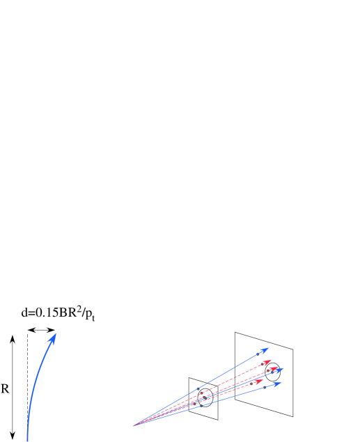
Figure 1.1: Cluster separation proportional to $BR^{2}$ (left), or proportional to $R^{2}$ (right).

The outer radius of the main tracker (TPC) is also large in GLD. Consequently the lever arm of the tracking is long and the number of sampling can be large. Therefore, we can expect an excellent momentum resolution for the charged particles ($\delta p_{t}/p_{t}^{2}\propto 1/BL^{2}\sqrt{n_{\rm{sample}}}$), and good particle identification ($\pi/K/p$) capability by $dE/dx$. The relatively low magnetic field of GLD is advantageous for the track reconstruction of low $p_{t}$ charged particles, and subsequently for vertex-charge determination, PFA, and so on.

1.1.3 Baseline Design

Figure 1.2 shows a schematic view of two different quadrants of the baseline design of GLD as of March 2006.

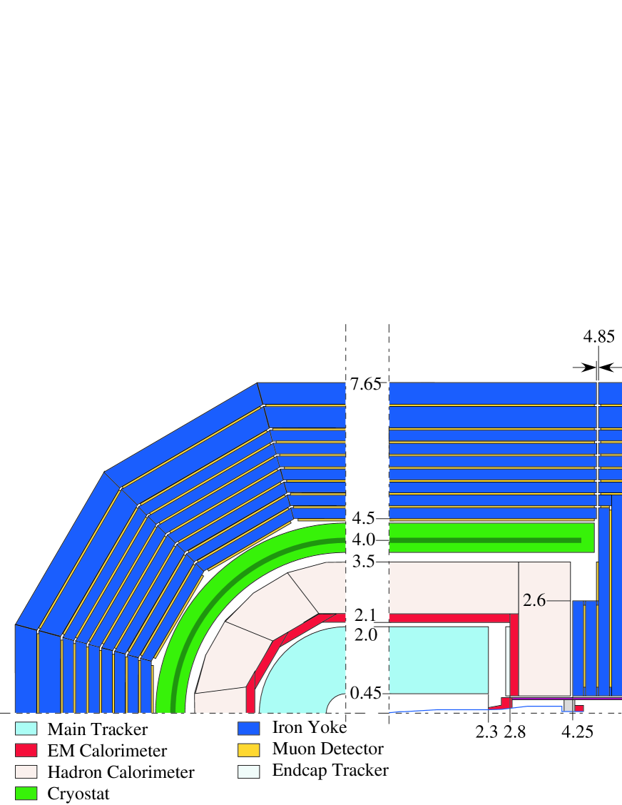
Figure 1.2: Schematic view of two different quadrants of GLD Detector. The left figure shows the $r\phi$ view and the right shows the $rz$ view. Dimensions are in meter. The vertex detector and the silicon inner tracker are not shown here.

The inner and forward detectors are schematically shown in Figure 1.3. The baseline design has the following sub-detectors:

• a large gaseous central tracker, presumably TPC,

• a large-radius medium/high-granularity ECAL with tungsten-scintillator sandwich structure,

• a large-radius thick ($\sim 6\lambda$) medium/high-granularity HCAL with lead-scintillator sandwich structure,

• forward EM calorimeters (FCAL and BCAL) down to 5 mrad,

• a precision silicon micro-vertex detector,

• silicon inner (SIT) and endcap(ET) trackers,

• a beam profile monitor in front of BCAL,

• a muon detector interleaved with iron plates of the return yoke, and

• a moderate magnetic field of 3 T.

The iron return yoke and barrel calorimeters have dodecagonal shape (24-sided shape for the outside of HCAL) rather than octagonal shape in order to reduce unnecessary gaps between the muon system and the solenoid, between HCAL and the solenoid, and between TPC and ECAL.

In addition to the baseline configuration, the following options are being considered. Silicon tracker between TPC and EM calorimeter in the barrel region is proposed to improve the momentum resolution still more. It is also suggested that a TOF counter in front of the EM calorimeter can improve the particle identification capability, but this function could be included in the EM calorimeter.

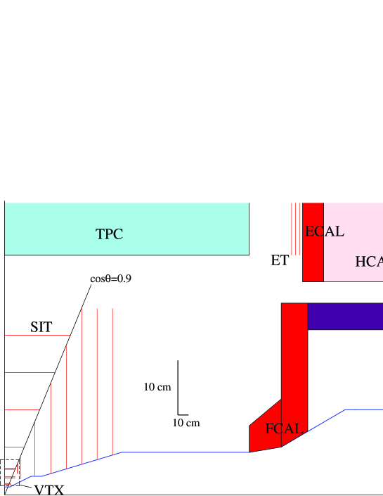
Figure 1.3: Schematic view of the inner and forward detectors of GLD. The horizontal scale and the vertical scale is not same as indicated in the midle of the figure.

MDI (Machine Detector Interface) issues, as well as the physics requirements, give impact on the detector design. Beam background has to be taken into account for the design of ILC detectors. The beam pipe radius and inner radius of the vertex detector of GLD have been determined based on the consideration of pair background (see Section 2.1). The configuration of FCAL and BCAL of GLD has been chosen so that the back-scattered photons produced by the dense core of pair background at BCAL do not hit the TPC drift volume directly.

There are three options for the beam crossing angle; 2 mrad, 14 mrad, and 20 mrad. In case of 20 mrad crossing angle, a dipole magnetic field could be implemented inside the detector in order to cancel the transverse field component of the solenoid magnet for the incoming beam and make the electron and positron beams collide vertically head-on. This dipole field could be produced by a so-called detector-integrated dipole (DID). Because DID doubles the transeverse field component for the outgoing beam, it could cause a background problem in SIT due to backscattering from BCAL. In case of 14 mrad crossing angle, use of anti-DID which has reverse polarity of the DID is considered to make the beams collide vertically head-on. In this case, SIT is free from the backscattering problem.

Another parameter which affects the detector design is $L^{*}$, the distance between the interaction point and the front surface of the final quadrupole magnet. We assume a large $L^{*}$ for GLD ($L^{*}=4.6$ m).

Time structure of the ILC beam gives impact on the requirment for the performances of some sub-detectors. Figure 1.4 shows the time structure of the ILC beam. In the nominal option of the ILC accelerator design, 2820 bunches of electrons and positrons make a train with 307.7 ns time intervals between bunches, and the trains are repeated at a rate of 5 Hz. In order to untangle the event overlap in one train, bunch-identification (time stamping) capability is necessary for the silicon trackers and calorimeters.

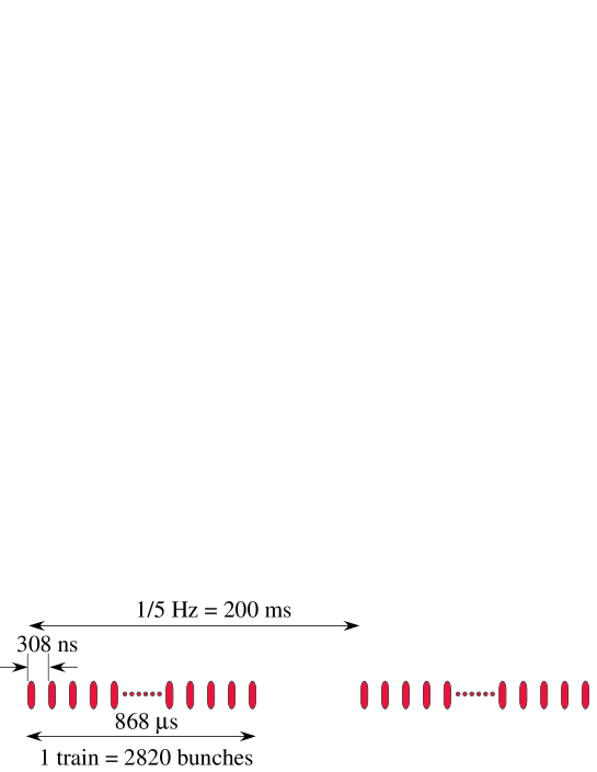
Figure 1.4: Time structure of the ILC beam.

The parameters of the detector and the sub-detector technologies of GLD are modified from time to time based on considerations on the detector performance, development of more realistic detector design, considerations on cost issue, requirements from accelerator side, and so on. It is unrealistic to do the simulation study again and again for every modifications. Therefore the detector model implemented in the detector simulator does not necessarily reflect all the modification of the baseline design. In this report, the detector model assumed in Chapter 3 (Sections on the performance) is based on an older version than what is described in Chapter 1 and Chapter 2. The cost estimation will be done based on the baseline design described in this section.

1.1.4 Overview of Sub-detectors

In this subsection, we will describe each sub-detector very briefly. The detail of the detector sub-system will be described in Chapter 2. The parameters of the sub-detectors are listed in Table 1.1 for trackers and in Table 1.2 for calorimeters. The parameters listed in this table are based on the latest baseline design and not necessarily consistent with the parameters given in Part 3 (Table 3.1).

Table 1.1: Parameters of trackers of GLD. The spatial resolutions are values to be implemented in the simulator and not necessarily segmentation size devided by $\sqrt{12}$. The thickness $t$ includes the support structure converted into silicon-equivalent thickness. The configuration of first two layers of VTX depends on the machine parameter option (see Section 2.1).

	$R$ (cm)	$Z$ (cm)	$\cos{\theta}$	$t$ ($\mu$m)	Resolution
	2.0	6.5	0.9558
	2.2	6.5	0.9472
	3.2	10.0	0.9524
VTX	3.4	10.0	0.9468	80	5 $\mu\rm{m}^{2}$ pixel
	4.8	10.0	0.9015		$\sigma=2\ \mu$m
	5.0	10.0	0.8944
	4.0–5.8	12.0	0.9003–0.9487
	4.0–5.8	12.2	0.9031–0.9502
	9.0	18.5	0.8992		R-$\phi$: 50 $\mu$m strip pitch,
BIT	16.0	33.0	0.8998	560	$\sigma=10\ \mu$m
	23.0	47.5	0.9000		$Z$: 100 $\mu$m strip pitch,
	30.0	62.0	0.9002		$\sigma=50\ \mu$m
	2.4–7.6	15.5	0.8979–0.9882
	3.2–14.0	29.0	0.9006–0.9940
	3.7–21.0	43.5	0.9006–0.9964
FIT	4.7–28.0	58.0	0.9006–0.9967	560	$\sigma=25\ \mu$m
	5.7–38.0	72.5	0.8857–0.9969
	6.6–38.0	87.0	0.9164–0.9971
	7.6–38.0	101.5	0.9365–0.9972
		270.0	0.7964–0.9864
ET	45.0–205.0	274.0	0.8007–0.9868	560	$\sigma=25\ \mu$m
		278.0	0.8048–0.9872
TPC	45.0–200.0	230.0	0.7546 (full)	–	$\sigma_{r-\phi}=50$–150 $\mu$m
			0.9814 (min)		$\sigma_{z}=0.5$ mm

Table 1.2: Parameters of calorimeters.

	$R$ (m)	$Z$ (m)	Structure	$X_{0}$	$\lambda$
ECAL	2.1 – 2.3	2.8	W/Scinti./gap	26	1.0
	0.4 – 2.3	2.8 – 3.0	3/2/1(mm) $\times 33$ layers
HCAL	2.3 – 3.5	3.0	Pb/Scinti./gap	165	5.7
	0.4 – 3.5	3.0 – 4.2	20/5/1(mm) $\times 46$ layers
FCAL	(0.08 – 0.36)	(2.3 – 2.85)	W/Si
BCAL	0.02 – 0.36	4.3 – 4.5	W/Si or W/Diamond

Vertex Detector

Very good impact parameter resolution for charged tracks is required at ILC for efficient jet-flavor identification. The target value of the impact parameter resolution is

$$\sigma_{b}=5\oplus\frac{10}{p\beta\sin^{3/2}{\theta}}\ (\mu m).$$

In order to achieve this resolution, the Si pixel vertex detector has to have excellent point resolution and thin wafer thickness.

For the baseline design of the vertex detector, we envisage fine pixel CCDs (FPCCDs) as the sensors. The inner radius is 20 mm and the outer radius is 50 mm. It consists of three layers of doublets where a doublet is made by two sensor layers with 2 mm distance.

In FPCCD option, pixel occupancy is expected less than 0.5% for the inner most layer (R=20 mm) at B=3 T for the ILC nominal machine parameters [6]. The hit density is, however, as high as 40/$\rm{mm}^{2}$. Therefore, very thin wafer (much less than 100 $\mu$m) is required in order to keep wrong-tracking probability due to multiple scattering reasonably low [7]. The R&D effort on the wafer thinning is very important, as well as the fabrication of the small pixel sensors.

Silicon Trackers

Silicon Inner Tracker

The silicon inner tracker is located between the vertex detector and main tracker. It consists of the barrel inner tracker (BIT) and the forward inner tracker (FIT).

The roles of the barrel inner tracker are to improve the linking efficiency between the main tracker and the vertex detector, and to reconstruct and measure momenta of low $p_{t}$ charged particles. Time stamping capability to separate bunches (307.7 ns or 153.8 ns interval) is necessary as well as good spatial resolution.

Silicon strip detectors will be used for the BIT. Four layers of silicon strips are being considered for stand-alone tracking capability. The innermost and outermost layers of the BIT are located at the radii of 9 cm and 30 cm, respectively.

Forward silicon tracker (FIT) should cover the angular range down to $\sim 150$ mrad which corresponds to the coverage of the endcap calorimeter. The technologies used for the FIT depends on the track density of jets and the background level (beam background and 2-photon background). Detailed simulation study is necessary to determine the technology. We assume silicon pixel sensors for the first three layers and silicon strip sensors for the other four layers.

Silicon Endcap Tracker

Several layers of silicon strip detectors are placed in the relatively large gap between the TPC and the endcap EM calorimeter. This endcap silicon tracker (ET) improves momentum resolution for charged particles which have small number of TPC hits. Another role of the ET is to improve matching efficiency between TPC tracks and shower clusters in the EM calorimeter. This function is important particularly for low momentum tracks.

Main Tracker

A large gaseous tracker will be used for GLD as the main tracker. In the baseline design, a TPC (Time Projection Chamber) with 40 cm inner radius and 200 cm outer radius is assumed. The maximum drift length in z-direction is 230 cm.

The requirement for the performance of the TPC in GLD is to achieve the momentum resolution of $\delta p_{t}/p_{t}^{2}<5\times 10^{-5}$ combined with the silicon inner tracker and the vertex detector at the high $p_{t}$ limit.

TPCs have been used in a number of large collider experiments in the past and have performed excellently. These TPCs were read out by multi-wire proportional chambers (MWPCs). The thrust of R&D is to develop a TPC based on novel micro-pattern gas detectors (MPGDs), which promise to have better point and two-track resolution than wire chambers and to be more robust in high backgrounds than wires. Systems under study at the moment are Micromegas[8] meshes and GEM (Gas Electron Multiplier)[9] foils. Both operate in a gaseous atmosphere and are based on the avalanche amplification of the primary produced electrons. The gas amplification occurs in the large electric fields in MPGD microscopic structures with sizes of the order of 50 $\mu$m. MPGD lend themselves naturally to the intra-train un-gated operation at the ILC, since, when operated properly, they display a significant suppression of the number of back-drifting ions.

Calorimeter

As mentioned in Section 1.1.2, the calorimeter of GLD should have large radius and fine 3D segmentation in order to get excelent jet energy resolution by PFA. The target value of the jet energy resolution is

$$\sigma(E_{j})/E_{j}=30\%/\sqrt{E_{j}(GeV)}.$$

EM Calorimeter

The EM calorimeter (ECAL) should have small effective Moliere length in order to suppress the shower spread and minimize the deterioration of the jet-energy resolution due to confusion of $\gamma$s and charged tracks. For this reason, tungsten will be used for the absorber material.

Because the size of EMCAL is quite large ($\sim 100\ \rm{m}^{2}$/layer), it may not be practical to use silicon pad as the sensor due to cost. Therefore, the baseline design adopts scintillator strips or tiles with wavelength-shifter fiber readout. As the photon sensor, the use of MPPC (Multi-Pixel Photon Counter) is considered. It consists of 30 sampling layers of tungsten/scintillator with the thicknesses of 3 mm/2 mm and 1 mm gap for readout. The effective segmentation cell size is 1 cm$\times$1 cm with orthogonal strips.

Hadron Calorimeter

The hadron calorimeter (HCAL) of GLD, as a baseline design, consists of 46 layers of lead/scintillator sandwiches with 20 mm/5 mm thickness and 1 mm gap for readout. This configuration is thought as a “hardware compensation” configuration which gives the best energy resolution for a single particle. The effective cell size is 1 cm square to be achieved by 1 cm  x 20  cm strips and 4  cm  x 4 cm tiles. As the photon sensor, the use of MPPC is considered to read scintillating lights through a wave length shifting fiber. Another option of “digital hadron calorimeter” is also considered for HCAL so as to reduce the cost of read out electronics. For the digital HCAL, the base line design consists of scintillator strip may have shower overlap problem. With a realistic PFA model, we need to clarify this, so as to determine the optimal width and length of the strips.

Forward Calorimeters

The forward calorimeter of GLD consists of two parts: FCAL and BCAL. The z-position of FCAL is close to that of endcap ECAL, and it locates outside of the dense core of the pair background in R direction. BCAL is located just in front of the final quadrupole magnet ($\sim 4.5$ m). The inner radius of FCAL and BCAL depends on the machine parameters. In case of small crossing angle of 2 mrad, the inner radius of the BCAL can be as small as 20 mm and the minimum veto angle for the electrons of 2-photon processes is $\sim 5$ mrad.

Since BCAL is hit by the dense core of the pair background, it creates a lot of backscattered $e^{\pm}$ and photons. A mask made by low-Z material with the same inner radius as the BCAL should be put in front of BCAL to absorb low energy backscattered $e^{\pm}$. The z-position of FCAL should be chosen so that FCAL works as a mask for the backscattered photons from BCAL and they cannot hit TPC directly.

Technology of FCAL and BCAL is still open question. For FCAL, W/Si sampling calorimeter will work well. For BCAL, more radiation hard sensors, such as diamond, would be the option.

Muon System

The muon detector of GLD is not required to work as a tail catcher, because calorimeters of GLD has the thickness close to 7 interatcion length which is thick enough to contain hadron showers. Therefore, the baseline design of GLD has just 9 or 10 layers of muon detectors interleaved with the iron return yoke, each layer being consists of two-dimensional array of scintillator strips with wavelength-shifter fiber readout by MPPC.

Detector Magnet and Structure

The detector magnetic field is generated by a super-conducting solenoid with correction winding at both ends. The radius of the coil center is 4.0 m and the length is 8.9 m. Additional serpentine winding for the detector integrated dipole (DID) might be necessary to compensate the radial component due to finite crossing angle. The integrated field uniformity at the tracker region with this configuration satisfies

$$\biggl{|}\int_{0}^{z_{max}}\frac{B_{r}}{B_{z}}dz\biggr{|}<2~{}\rm{mm}$$

without DID. This value is good enough for TPC. The total size of the iron structure has a height of 15.3 m and a length of 16 m. The thick iron return yoke is required to keep leakage field low enough. The requirement for the leakage field from the accelerator side is less than 50 Gauss on the beamline at $z=10$ m.

Data Aquisition

The main goal of the data acquisition (DAQ) system is to take data of interesting events efficiently in the presence of several orders of magnitude higher backgrounds. Although the minimum bias event rates are expected to be lower than the hadron colliders, the data size will be large due to the huge readout channels to measure physics processes with the required accuracy. The bunch structure of the ILC operation conditions leads to the proposal of an event building system without any hardware trigger and of some pipelinings to achieve a dead-time free DAQ system.

Since the DAQ system depends on the final design and also on the rapid development of the technologies, the system presented here is still conceptual, showing possible options and technologies forecast.

1.1.5 Optional Sub-detectors

Silicon Outer Tracker

The performance goal of the tracking system has long been thought as $\delta p_{t}/p_{t}^{2}=5\times 10^{-5}$ at high $p_{t}$ limit [5]. This value comes from a consideration of Higgs mass measurement error in $e^{+}e^{-}\rightarrow ZH,\ Z\rightarrow\mu^{+}\mu^{-}$ that the error should be dominated by beam energy spread and beam strahlung. Recently, however, reconsideration based on new beam parameters suggests better resolution than $5\times 10^{-5}$ could give better physics outputs. In order to get better momentum resolution, putting a high resolution silicon tracker outside the TPC in the barrel region is an option of GLD. The performance and feasibility of this option should be studied in case the better momentum resolution is required.

Particle Identification

Determination of heavy quark sign (quark-antiquark tag) plays an important role in physics study at ILC. Measurement of angular distribution and left-right asymmetry in $e^{+}e^{-}\rightarrow b\ \bar{b}$ could reviel the existence of extra dimension [10]. Differential cross setion of $e^{+}e^{-}\rightarrow\tilde{\chi}^{+}_{1}\tilde{\chi}^{-}_{1}$ has to be measured to study the property of chargino, and charge of charm and bottom quark in $\tilde{\chi}^{\pm}_{1}\rightarrow W^{\pm}\tilde{\chi}^{0}_{1}$, $W^{\pm}\rightarrow c\ \bar{b}$ or $\bar{c}\ b$ has to be measured to determine the sign of the mother chargino. Vertex charge measurement is an approach widely used at SLD and LEP experiments. However, kaon charge identification would increase the efficiency significantly.

In GLD, $K/\pi$ separation can be achieved to some extent by $dE/dx$ measurement in the TPC. Recently $dE/dx$ resolution better than 3% was suggested using “digital TPC”. If this resolution is realized, we will have a fairly good efficiency in $K/\pi$ separation above 2 GeV/c. However, there is an efficiency gap between 0.9 GeV/c and 2 GeV/c in $K/\pi$ separation by $dE/dx$. This gap can be filled by TOF measurement in front of ECAL with a resolution of $\sim 100$ ps. If efficiency loss due to this gap is non-negligible, the first layer of ECAL should have the TOF measurement capability.

Chapter 2 Detector Sub-systems

2.1 Vertex Detector

2.1.1 Introduction

In order to achieve the performance goal of $\sigma_{b}=5\oplus 10/p\beta\sin{\theta}^{3/2}$ $\mu$m, the vertex detector should have very thin layer thickness ($<100\ \mu$m/layer) and small inner radius. Compared with other two detector concepts, GLD has relatively low magnetic field of 3 T (LDC and SiD have 4 T and 5 T, respectively). The impact of the magnetic field on the vertex detector design is the radius of the innermost layer. Higher magnetic field confines the pair-background in a smaller radius, and the beam pipe and the vertex detector can be put closer to the beam line. So the GLD vertex detector has to have slightly larger inner radius $R_{VTX}$ to keep background hit density same as other detector concepts.

At ILC, 2820 bunches of electron and positron beam make collisions successively with 307.7 ns bunch intervals. This succession of 2820 bunches is called “train”, and trains are repeated at a rate of 5 Hz. Due to low energy electron/positron beam background, the hit rate of the innermost layer of the vertex detector is estimated to be $\sim 1.5\rm{\ hit/cm^{2}}$ at R=2.0 cm and B=3 T for one bunch crossing (BX). If the hits are accumulated for one train, the hit density becomes very high, and the pixel occupancy for a pixel detector with 25 $\mu$m pixel size exceeds 10%, which is not acceptable.

One method to keep the pixel occupancy acceptable level ($\sim 0.5$%) is to read out the sensors more than 20 times in one train. Another method is to increase the number of pixels by factor of $\sim 20$ useing very fine pixels. In this fine pixel option, the data can be read out in 200 ms interval between trains and very fast readout is not necessary.

2.1.2 Baseline Design

Fine Pixel CCD

As the vertex detector for the ILC experiment, a lot of sensor technologies are proposed but non of them seems to be demonstrated to work satisfactorily at ILC. For the moment, we assume fine pixel CCD (FPCCD) option for the baseline design of the GLD vertex detector. It does not mean that the standard pixel options are rejected for GLD, of course.

For the FPCCD vertex detector [11, 12], we use very fine ($\sim 5$ $\mu$m) pixel CCDs. By increasing the number of pixels by a factor of about 20 compared with standard pixel sensors, the pixel occupancy will be less than 1% even if the hit signal is accumulated during a whole train of 2820 bunches. In order to suppress the number of hit pixels due to diffusion in the epitaxial layer, the sensitive layer of the FPCCD has to be fully depleted.

A big challenge of the FPCCD vertex detector is the high hit density due to pair-background hits. Although the pixel occupancy is satisfactorily low, the hit density is as high as 40 hits/$\rm{mm}^{2}$ at B=3 T and R=20 mm with the machine parameter of the “nominal option” [6]. This high hit density could cause tracking inefficiency if the multiple scattering effect is large. When a signal hit candidate on a layer is searched for by extrapolating signal hits of outer layers, the background hits cause misidentification probability $p_{mis}$. For a normal incident track, $p_{mis}$ is given by

$$p_{mis} = 2\pi\sigma R_{0}^{2},$$ (2.1)

$$R_{0} = d\theta_{0}$$

where $\sigma$ is background hit density of the inner layer, $d$ is the distance between inner and outer layers, and $\theta_{0}$ is the multiple scattering angle by the outer layer. The angular and momentum dependence of $p_{mis}$ is $p_{mis}\propto p^{-2}\sin^{-4}{\theta}$, where $p$ is the momentum and $\theta$ is the polar angle.

The misidentification probability for 1 GeV/c particles is plotted as a function of $\cos{\theta}$ in Figure 2.1 assuming the layer thickness of 50 $\mu$m Si. As can be seen from this figure, misidentification probability quickly goes up in the forward region. If the distance between inner two layers is 10 mm, $p_{mis}$ is nearly 30% at $\cos{\theta}=0.95$ with the background hit density of $40/{\rm mm}^{2}$. To reduce the misidentification probability, the distance between inner two layers should be small. If the distance is 2 mm, $p_{mis}$ is as small as the case of $d=10$ mm and $\sigma=2/{\rm mm}^{2}$, which is expected when the sensor is read out 20 times per train.

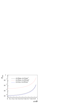
Figure 2.1: Misidentification probability of signal hit with background hit as a function of $\cos{\theta}$ for several layer configurations. The layer thickness of 50 $\mu$m and the particle momentum of 1 GeV/c are assumed.

Another way to reduce $p_{mis}$ more is background rejection using hit cluster shape of the FPCCD. The momentum spectrum of the pair-background particles hitting the innermost layer of the vertex detector has a peak around 20 MeV/c at 3 T magnetic field. Therefore, the incident $\phi$ angle of background particles to the sensor plane is quite different from that of large $p_{t}$ signal particles. As a consequence, the hit clusters of background particles have larger spread in $\phi$ direction and smaller spread in $z$ direction than what is expected for the large $p_{t}$ particles as shown in Figure 2.2. Background rejection of about factor 20 is expected for large $\cos{\theta}$ region where the misidentification probability becomes large [12].

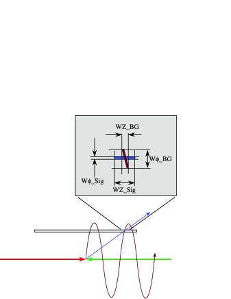
Figure 2.2: Hit cluster shape of a high $p_{t}$ track (blue) and a pair-background track(brown).

Layer Configuration

The baseline design of the vertex detector is schematically shown in Figure 2.3. Two sensor layers put in proximity make a doublet to reduce the misidentification probability.

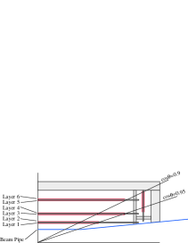
Figure 2.3: Schematic design of the FPCCD vertex detector.

CCD wafers will be thinned down to 50 $\mu$m and glued on both sides of 2-mm-thick plates made of rigid foam such as reticulated vitreous carbon (RVC) foam or silicon carbide (SiC) foam. The density of RVC can be as small as 3% of graphite, which corresponds to 0.016%$X_{0}$ for 1 mm thickness.

The angular coverage is $\cos{\theta}<0.9$ with 6 barrel layers and $\cos{\theta}<0.95$ with 4 barrel layers plus 2 forward-disk layers. Because we need end-plates with sizable material budget to support barrel laddes, the role of the forward-disk layers may be less important for low momentum tracks. The whole ladders are supported from outer shell made by berylium or CFRP, and confined in a cryostat made by low-mass material (polystyren foam for example). The CCDs are operated at low temperature in order to keep dark current and charge transfer inefficiency due to radiation damage reasonably low.

The inner radius of the vertex detector is determined by a consideration on beam background. We have estimated the possible smallest radii of the beam pipe and the innermost layer of the vertex detector based on a simple model. The model we have used is shown in Figure 2.4. The minimum radii of the beam pipe and the first layer of the vertex detector were determined using following design criteria:

• The dense core of the pair background should not hit the beam pipe. It should have $\sim 5$ mm clearance at $z=350$ mm and $\sim 2$ mm clearance at the junction of the central beryllium part and the conical part.

• The silicon wafer is 2 mm longer than what is required to cover $|\cos{\theta}|<0.95$.

• The ladder length is longer than the silicon wafer by 15 mm. The clearance between the ladder and the conical part of the beam pipe is 2 mm.

The simulation for pair background was done using CAIN for various ILC parameter sets. The track density of the pair background in $z$-$r$ plane is shown in Figure 2.5 with the nominal ILC parameter set [6] and crossing angle of 2 mrad for 3, 4, and 5 T magnetic field. Figure 2.6 shows the track density distribution for high luminosity option of ILC parameters [6]. The distribution of the dense core of the pair-background tracks with the original high luminosity option is significantly broader than that with the nominal option. Recently, A. Seryi proposed new high-luminosity parameter sets [13]. These new high luminosity parameter sets give less and narrower pair background as can be seen from Figure 2.6.

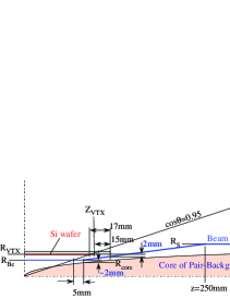
Figure 2.4: Model for estimation of radii of the beam pipe and innermost layer of the GLD vertex detector.

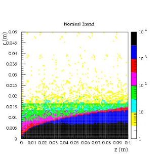
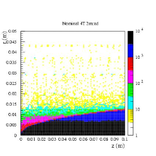
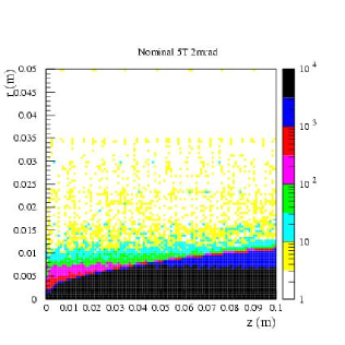
Figure 2.5: Pair-background track density ($/\rm{cm}^{2}/\rm{BX}$) with the nominal ILC machine parameter at 500 GeV and 2 mrad crossing angle in 3 T (left), 4 T (center), and 5 T (right) magnetic field.

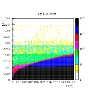
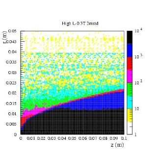
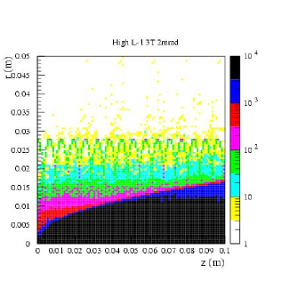
Figure 2.6: Pair-background track density ($/\rm{cm}^{2}/\rm{BX}$) with the high luminosity option of ILC machine parameter at 500 GeV (left), 1 TeV (center) [6], and the new high luminosity option at 1 TeV [13] (right). The crossing angle is 2 mrad and the magnetic field is 3 T for all three cases.

The beam-pipe parameters and minimum radius of the vertex detector $R_{VTX}$ determined by the design criteria and the background simulation described above are summarized in Table 2.1. We can see that minimum $R_{VTX}$ strongly depends on the machine parameter option.

Table 2.1: The beam-pipe parameters and minimum $R_{VTX}$ for several machine options and different magnetic field $B$ based on a certain design criteria. High Lum-A1 and High Lum-A2 stand for the new high luminosity parameter sets proposed by A. Seryi. See Figure 2.4 for the definition of each parameter.

$E_{CM}$	Option	B (T)	$R_{core}\ (mm)$	$R_{Be}\ (mm)$	$R_{VTX}\ (mm)$
500 GeV	Nominal	3	10.5	12.5	16.6
		4	9	11	14.9
		5	7.5	9.5	13.2
	High Luminosity	3	16.5	18.5	24.1
		4	13.5	15.5	20.2
		5	12	14	18.4
1 TeV	Nominal	3	11	13	17.3
	High Luminosity	3	18.5	20.5	25.8
	High Lum-A1	3	13	15	19.4
	High Lum-A2	3	11.5	13.5	17.8

From this study, we choose the radii of Be beam pipe ($R_{Be}$) and innermost layer of the vertex detector ($R_{VTX}$) as 15 mm and 20 mm, respectively, as the baseline. We also considered two options for different background conditions as listed in Table 2.2. The baseline configuration can be used even for High-Lum-A1 option at 1 TeV. The “small-R” configuration can be used only for the nominal machine option at 500 GeV, and somewhat risky. The “large-R” configuration is compatible with the high luminosity option at 500 GeV.

Table 2.2: Design parameters of the beam pipe radius ($R_{Be}$), the radius ($R_{VTX}$) and the half length ($Z_{VTX}$) of the first layer of the vertex detector.

Configuration	$R_{Be}\ \rm{(mm)}$	$R_{VTX}\ \rm{(mm)}$	$Z_{VTX}\ \rm{(mm)}$
Baseline	15	20	65
Small R	13	17	55
Large R	19	24	75

Signal Readout

Each wafer of the FPCCD will have multi-port readout in order to reduce the readout time and to reduce the effect of charge transfer inefficiency (CTI) caused by radiation damage. A readout ASIC consisting of amplifiers, correlated double samplers, and analog-to-digital converters (ADCs) will be put on both ends of a ladder. Because the FPCCD option can achieve an excellent spatial resolution even with digital readout, few bits will be enough for the ADCs.

The data size of the vertex detector is dominated by the contribution from the pair-background hits. The total number of pixels is as large as $\sim 1\times 10^{10}$ (10 G pixels). If the pixel data is consisted of 34 bit address plus 5 bit analog data, the data size for 1% pixel occupancy becomes about 5 Gbits per train. Actually the pixel occupancy of the outer layers is much less than 1%, and the dada size will be much smaller than this vaue. The data size derived from the expected number of hits for the nominal option of the machine parameters is less than 0.5 Gbits per train. Therefore, a small number of optical fiber cables with few Gbps throughput will be enough for the data transfer.

2.1.3 Possible Options

In this report, we assume FPCCD as a technology for the vertex detector of the baseline GLD design, but this is just an assumption. There are a lot of candidate technologies studied all over the world. The options are; column parallel CCD (CPCCD), CMOS monolithic active pixel sensor (MAPS), depleted FET (DEPFET), pixel sensor based on SOI technology (SOI), CMOS pixel sensor with registers in each pixel (CAP/FAPS), in-situ storage image sensor (ISIS), and fine pixel CCD (FPCCD). Among them, CAP, FAPS, ISIS, and FPCCD accumurate the signal during a train and are read out in between trains.

The R&D efforts for these technologies will be continued for several years. The technology choice for the vertex detector in future will be done by real “collaboration groups” of the ILC experiment based on the results of the R&D.

2.1.4 R&D needed

Development of sensors and demonstration of their performance satisfying the requirements as the vertex detector for ILC experiments are the highest priority R&D issues for all sensor technologies. Study of wafer thinning technique and development of their support structure are also indispensable. Other R&D items are; development of the front-end readout ASIC, minimization of power consumption, data compression and the back-end electronics, cooling system with minimum material, and development of thin beam pipe.

2.2 Silicon Inner Tracker

2.2.1 Detector Features

The silicon inner tracker (SIT) is considered to improve a momentum resolution and reconstruction efficiency of long-lived particles with the vertex detector and help pattern recognition in linking the tracks found in the Time Projection Chamber (TPC) with the tracks found in the vertex detector. The SIT consists of the barrel inner tracker (BIT) in the barrel region and the forward inner tracker (FIT) in the endcap region. Four cylindrical BIT layers are located between the vertex detector and the TPC (Figure 1.3).

The four layers will consist of the double-sided silicon strip detectors with 10 $\mu$m spatial resolution in r$\phi$ direction. Seven plane disks perpendicular to the beam direction are positioned as the FIT. The four inner planes with any pixel-based sensors and the remaining three planes with silicon strip detectors (modest resolution) are being considered. The SIT design of the BIT and the FIT is shown in Figure 2.7.

Table 2.3: Parameters for the BIT.

BIT	half Z(cm)	R(cm)	sensor size(cm2)
layer1	18.5	9	5 $\times$ 5
layer2	33.0	16	5 $\times$ 5
layer3	47.5	23	5 $\times$ 5
layer4	62.0	30	9 $\times$ 9

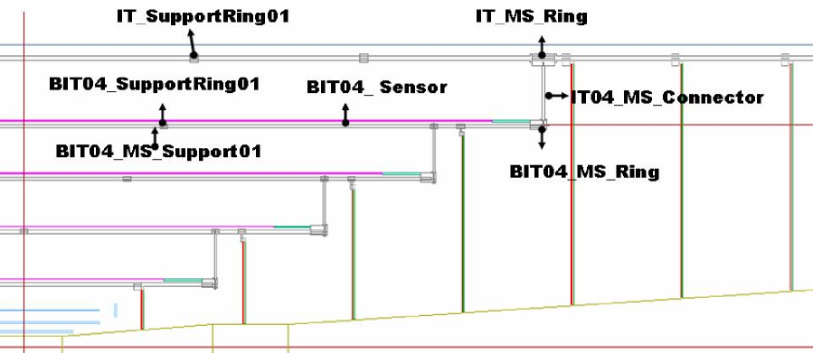
Figure 2.7: A layout of the silicon inner tracker (SIT) consisting of four cylindrical in the barrel (BIT) and seven planes in the endcap (FIT).

Some of key mechanical parameters associated with the BIT and FIT design are listed in Table  2.3 and Table  2.4, respectively.

Table 2.4: Parameters for the FIT.

BIT	half Z(cm)	Rmin(cm)	Rmax(cm)
layer1	15.5	2.4	7.6
layer2	29.0	3.2	14.0
layer3	43.5	3.7	21.0
layer4	58.0	4.7	28.0
layer5	72.5	5.7	38.0
layer6	87.0	6.6	38.0
layer7	101.5	7.6	38.0

2.2.2 Performance of the SIT

The SIT has been designed to have nearly the full solid angle coverage and stand alone track finding and reconstruction. The momentum resolution of the tracking system is required to be $5~{}\times~{}10^{-5}~{}$(GeV/c)^-1 [3]. The resolutions of $7~{}\times~{}10^{-5}~{}$(GeV/c)^-1 for the vertex detector alone and $1.4~{}\times~{}10^{-4}~{}$(GeV/c)^-1 for the TPC alone are achievable and the addition of the silicon layers in the space between the vertex and the TPC detectors improves the resolution to the required precision of $5~{}\times~{}10^{-5}~{}$(GeV/c)^-1 as shown in Figure 2.8.

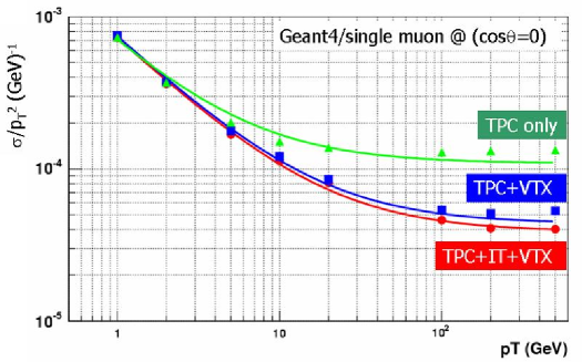
Figure 2.8: Momentum resolution as a function of the momentum for a polar angle $\theta$ = $90^{\circ}$ of single muon for different combination of subdetector.

The multiple Coulomb scattering is dominant in the low momentum region and addition of the SIT does not help to improve the momentum resolution.

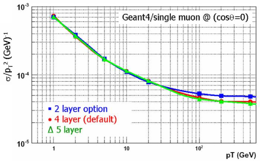
Figure 2.9: Momentum resolution as a function of transverse momentum for the different number of layers option in SIT.

Figure 2.9 shows the momentum resolution as a function of the momentum for the different number of layers in the SIT and the simulation result shows that four layers is reasonable choice to achieve the required momentum resolution.

The linking and reconstruction efficiency of charged tracks from physics events should be studied. Since the angular resolution in the detector performance is important in the endcap regions, the polar angular resolution as a function of the polar angle should be studied. This is important in the bremsstrahlung energy spectrum because error on the effective center of mass energy is given by error on collinearity distribution of Bhabha events.

2.2.3 Technologies

The Double-sided Silicon Strip Detector (DSSD) will be used for the BIT and 10 $\mu$m resolution in r$\phi$ is required. The SIT consist of 4 layers of DSSD. Since z measurement is needed to improve the track finding efficiency, 50 $\mu$m resolution in z is largely sufficient. The physical dimension of the sensor will be 50mm $\times$ 25mm with 300 $\mu$m thickness. There will be 511 $n^{+}$ strips with 50 $\mu$m pitch, and 511 $p^{+}$ strips with 100 $\mu$m pitch. This type of the DSSD sensors [16] are already used for the silicon vertex detectors in high energy experiments [17].

The inner four planes and the outer three planes of the FIT will consist of pixel and strip detectors, respectively. Among the silicon pixel sensor technology, ATLAS pixels with a pixel of 50 $\mu$m $\times$ 300 $\mu$m can be used [14]. The requirements of the strip detectors for the FIT are somewhat loose compared with those for the BIT. 25 $\mu$m resolution is required and this resolution can be achieved with a strip pitch of 100 $\mu$m and a readout pitch of 300 $\mu$m.

2.2.4 Detector Conceptual Designs

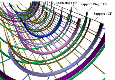
Figure 2.10: A conceptual layout of the BIT and FIT support structure. The space frame and the support ring consist of carbon fiber struts. The support shell and the support legs are made from composite materials.

Figure 2.10 shows a conceptual layout of a possible mechanical support structure. In this design we have to consider that the SIT is not only mechanically very rigid but also as thin as possible. The readout electronics will be located at the very end of the BIT layers in order to minimize the material in front of the TPC. The SIT is mechanically independent of the TPC and the whole TPC can be withdrawn from the detector.

In a recent measurement it has been shown that the Lorentz angle in silicon causes a broadening of the clusters of about 180 $\mu$m for electrons and about 40 $\mu$m for holes for 300 $\mu$m thick detectors and a magnetic field of 3 T if the strip are parallel to the B-filed. Not to be limited by this effect one has to use the p-side of the detectors for the r$\phi$-measurement and the n-side for z. Table 2.5 shows parameters in the conceptual design of the BIT.

Table 2.5: The number of channels between sensor types.

BIT	sensor area	# of sensor in a ladder	# ladder	# sensor	total area(mm2)
layer1	50 $\times$ 50	4	24	96	240000
layer2	50 $\times$ 50	7	48	336	840000
layer3	50 $\times$ 50	10	64	640	1600000
layer4	90 $\times$ 90	7	24	168	1360800

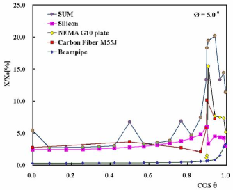
Figure 2.11: Material in units of radiation lengths as a function of the polar angle up to the end of the vertex detector and SIT.

With the assumption of overlap of 1.6 mm between neighboring detectors and silicon sensor size of 5 $\times$ 5 cm or 9 $\times$ 9 cm, the total number of sensors in a ladder on each layer and total number of sensors in a layer are given. In the pixel planes of the FIT electronic detectors of 0.5 cm² are bonded to a detector chip allowing great flexibility in the layout of the modules. In the strip planes of the FIT the strip disks are preferably built with double-sided detectors to minimize the material. The material budget as a function of the polar angle up to the end of the SIT is shown in Figure 2.11

2.2.5 R&D Program and Needed

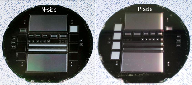
Figure 2.12: P-side and N-side of DSSD and test patterns.

The R&D program of the DSSD with DC-type is ongoing and AC-type is just started. Also single sided silicon strip sensors are under study. The DC-type of DSSD design is as follows. The sense strips on one side of the layer are orthogonal to the ones on the other side. This way one plane measures x and y coordinates of point, where ionizing particle goes through, on its two different sides [15]. The p-side has two metal layers; one layer for implantation strip and one for readout strip. The each of sensor side consists of 512 sensor strips with 50 $\mu$m and 100 $\mu$m pitch on n-side and p-side, respectively. Each strip is bias strip and the readout pads are made large for bonding. The sensor size has an area of 13.3 cm² and 2.6 cm long readout strips.

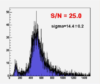
Figure 2.13: Signal to noise ratio of DSSD with ⁹⁰Sr beta source.

Two batches of 25 wafers were processed in ETRI [18] on 127 mm diameter, FZ, 380 $\mu$m thick, $<$100$>$-oriented, n-type silicon wafers, with resistivity of $>$ 5 k$\Omega$cm. A total of 11 masks steps were needed for the sensor fabrication process: 5 and 6 masks for n-side and p-side, respectively. To make the junction depth of the n -side deeper we started with n⁺ implantation and then p⁺ implantation is followed and Si₃N₄ instead of SiO₂ is employed as the isolation material at the second batch run. Figure 2.12 shows pictures of the n-side and p-side of the fabricated double-sided silicon strip sensors which are fabricated in 5-inch fabrication line in Korea. The leakage current and capacitance of the prototype strip sensor is being measured. It shows that the leakage current level of the single strip sense is from 8nA$-$20nA up to the full depletion voltage and values of the bulk leakage current level and the capacitance are about 1 $\mu$A and 50 pF, respectively. This measurement provides us information of the bulk characteristics and quality of the fabricated sensor.

We used ⁹⁰Sr beta source for the radioactive source test purpose. After the full depletion voltage was applied for the prototype, we measured the beta source signal with test readout electronics. We measured noise level of the silicon sensor without the beta source and the beta source is then put on the top of the silicon sensor in a dark box. The beta source signal was clearly seen and signal to noise is obtained to be 25 as shown in Figure 2.13.

The full R&D of the AC-type of DSSD and single sided silicon strip is necessary. Also comparison between the DC-type and AC-type should be done. The VA-chip was used for current R&D for the front-end readout electronics. However, it can’t be used for the ILC environment. We need to study which front-end readout ASIC is fit for the SIT. Also zero suppression and back-end electronics need to be studied.

2.3 Main Tracker

A Time Projection Chamber is chosen as central tracker for the GLD detector concept at the ILC. An R&D program is underway to develop the technology and prove the feasibility of a high-performance TPC required for this application. The use of new micro-pattern gas devices (MPGD) is an attractive possibility for the gas amplification. The decision for using an MPGD device, either the Gas Electron Multiplier (GEM) or the Micromegas technique, has included a comparison with the multi-wire proportional chamber (MWPC) technology used in past TPCs in a number of large collider experiments. For future TPCs, the MPGD technology promises to have better point and two-track resolution than wire chambers and to be more robust in high backgrounds.

2.3.1 The Basic Concept of the LC-TPC

General arguments for a TPC as main tracker are as follows.

• The tracks can be measured with a large number of ($r\phi$,$z$) space points, so that the tracking is continuous and the efficiency remains close to 100% for high multiplicity jets and in presence of large backgrounds.

• It presents a minimum of material to particles crossing it. This is important for getting the best possible performance from the electromagnetic calorimeter, and to minimize the effects due to the $\sim$10³ beamstrahlung photons per bunch crossing which traverse the detector.

• The comparatively moderate $\sigma_{singlepoint}$ and double-hit resolution are compensated by the continuous tracking and the large volume which can be filled with fine-granularity coverage.

• The timing is precise to 2ns (corresponding to 50 $\mu$m/ns drift speed of tracks hooked up to the $z$-strips of a silicon inner detector with 100$\mu$m pitch), so that tracks from different bunch crossings or from cosmics can readily be distinguished via time stamping.

• To obtain good momentum resolution and to suppress backgrounds near the vertex, the TPC has to operate in a strong magnetic field. It is well suited for this environment since the electrons drift parallel to $\vec{B}$, which in turn improves the two-hit resolution by compressing the transverse diffusion of the drifting electrons (FWHM${}_{T}\leq$ 2 mm for Ar-10%CH₄ gas and a 3T magnetic field).

• Non-pointing tracks, e.g. for V⁰ detection, are an important addition to the particle flow measurement and help in the reconstruction of physics signatures in many standard-model-and-beyond scenarios.

• The TPC gives good particle identification via the specific energy loss, dE/dx, which is valuable for many physics analyses, electron-identification and particle-flow applications.

• The TPC will be designed to be robust and at the same time easy to maintain so that an endplate readout chamber can readily be accessed or exchanged in case of accidents like beam loss in the detector.

Two additional properties of a TPC will be compensated by proper design.

• The readout endplanes and electronics present a small but non-negligible amount of material in the forward direction. The goal is to keep this below 30%X₀.

• The $\sim$50$\mu$s memory time integrates over background and signal events from 160 ILC bunch crossings at 500 GeV for the nominal accelerator configuration. This is being compensated by designing for the finest possible granularity: the sensitive volume will consist of several$\times 10^{9}$ 3D-electronic readout voxels (two orders of magnitude better than at LEP). It has been estimated to result in an occupancy of the TPC of less than $0.5\%$ from beam backgrounds and gamma-gamma interactions[3]. (See below for further discussion.)

2.3.2 Design issues.

There are many aspects for the layout of the LC detector and its subdetectors. The detector has to be designed globally to cover all possible physics channels, and the roles of the subdetectors in reconstructing many of these channels are highly interconnected. For the TPC, the issues are performance, size, endplate, electronics, gas, alignment and robustness in backgrounds.

Resolution expected/needed

The requirements for a TPC at the ILC are summarized in Table 2.6.

Table 2.6: Typical list of performance requirements for a TPC at the ILC detector.

Size	$\phi=4.1$m, L $=4.6$m
Momentum resolution	${\delta(1/{p_{t}})}\sim 10^{-4}$/GeV/c (TPC only; $\times$ 2/3 when IP included)
Solid angle coverage	Up to at least $\cos\theta\sim 0.98$
TPC material budget	$<0.03{\rm X}_{0}$ to outer field cage in $r$
	$<0.30{\rm X}_{0}$ for readout endcaps in $z$
Number of pads	$\sim$ 1.3$\times$106 per endcap
Pad size/Number of pad rows	$\sim$ 1mm$\times$6mm/$\sim$200
$\sigma_{\rm singlepoint}$ in $r\phi$	$\sim 100\mu$m (average over driftlength)
$\sigma_{\rm singlepoint}$ in $rz$	$\sim 0.5$ mm
2-track resolution in $r\phi$	$<2$ mm
2-track resolution in $rz$	$<5$ mm
dE/dx resolution	$<4.5$ %
Performance robustness	$>$ 95% tracking efficiency (TPC only), $>$ 98% overall tracking
Background robustness	Full precision/efficiency in backgrounds of 10-20% occupancy,
	whereby simulations estimate $<0.5$% for nominal backgrounds.

The main question to answer is: what should the resolution be for the overall tracking? This will define how many silicon layers are needed. According to various studies, that overall momentum resolution of ${\delta(1/{p_{t}})}\sim 5\times 10^{-5}$/GeV/c will be sufficient, as defined mainly by the e⁺e^-$\rightarrow HZ\rightarrow H\ell\ell$ channel used for measuring the Higgs production rate (see ref.[5], for example).

This resolution is achievable with inner-silicon tracking and a TPC performance given in Table 2.6. If for physics reasons, the overall tracking accuracy should be better, a larger TPC and/or more silicon layers should be envisaged[19].

Endplate

As stated in the introduction, MPGDs are the default technologies for the gas amplification since they promise better performance than the MWPC. Systems mainly under study are Micromegas [8] meshes and GEM [9] foils. Both[20] operate in a gaseous atmosphere and are based on the avalanche amplification of the primary produced electrons. The gas amplification occurs in the large electric fields within the MPGD microscopic structures with sizes of the order of 50$\mu$m. MPGDs lend themselves naturally to the intra-train un-gated operation foreseen for the ILC, since, when configured properly, they display a significant suppression of the number of back-drifting ions. In addition a gating plane will be foreseen for inter-train gating in order to have a safety factor in case of unexpected backgrounds (see below).

The two TPC endplates have a surface of about 10 m² of sensitive area each. The layout of the endplates, i.e. conceptual design, stiffness, division into sectors and dead space, has been started, for instance as shown in Figure 2.14.

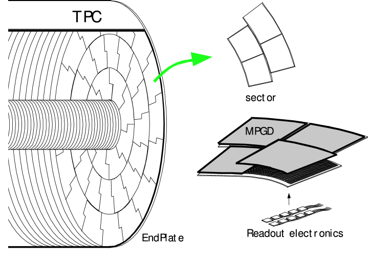
Figure 2.14: Ideas for the layout of the TPC endplates.

In this example the question arises as to how to make odd-shaped MPGDs if needed. In general, the readout pads, their size, geometry and connection to the electronics and the cooling of the electronics, are all highly correlated design tasks related to the endplates. As stated in Section 2.3.1, the material budget for the endcap and its effect on ECAL for the particle-flow measurement in the forward direction must be minimized. More details are covered in the next item.

Electronics

For the readout electronics, one of the important issues is the density of pads that can be accommodated while guaranteeing a thin, coolable endplate. The options being studied are (a) a standard readout (meaning, as in previous TPCs) of several million pads or (b) a pixel readout of a few hundred times more by using CMOS techniques.

(a) Standard readout:
Pad sizes under discussion are, for example, 2 mm times 6 mm (the TDR size[3]) or 1 mm times 6 mm which has found to be better as a result of our R&D experience (see below). A preliminary look at the FADC-type approach using 130 nm technology indicates that even smaller sizes like 1 mm times 1 mm might be feasible (in which case charge-spreading would not be needed). In all of these cases there are between 1.5 and 20 million pads to be read out. An alternative to the FADC-type is the TDC approach (see [21][22]) in which time of arrival and charge per pulse (via time over threshold) is measured. In case the material budget requires larger pads, then the resistive-foil technique[23] is an option to maintain the point resolution.

(b) CMOS readout:
A new concept for the combined gas amplification and readout is under development. In this concept[21] the MPGD is produced in wafer using post-processing technology on top of a CMOS pixel readout chip, thus forming a thin integrated device of an amplifying grid and a very high granularity endplate, with all necessary readout electronics incorporated. This concept offers the possibility of pad sizes small enough to observe individual single electrons formed in the gas and count the number of ionization clusters per unit track length, instead of measuring the integrated charge collected. Initial tests using Micromegas[24] and GEM foils[25] mounted on the Medipix2 chip provided 2-dimensional images of minimum ionizing track clusters. A modification of the Medipix2 chip (called Timepix) to measure also the drift time is under development[22]. Also a first working integrated grid has been produced[26].

Chamber gas

This issue involves (a) gas choice, (b) ion buildup and (c) ion feedback.

(a) Gas Choice
The choice of the gas for a TPC is an important and central parameter. Gases being investigated are variations of standard TPC gases, e.g.,
           Ar(93%)CH₄(5%)CO₂(2%)–“TDR” gas,
           Ar(95%)CH₄(5%)–“P5” gas,
           Ar(90%),CH₄(10%)–“P10”,
           Ar (90%)CO₂(10%),
           Ar (95%)Isobutane(5%) and
           Ar(97%)CF₄(3%).

When choosing a gas a number of requirements have to be taken into account. The $\sigma_{\rm singlepoint}$ resolution achievable in $r\phi$ is dominated by the transverse diffusion, which should be as small as possible. Simultaneously a sufficient number of primary electrons should be created for the point and dE/dx measurements, and the drift velocity at a drift field of a few times 100 V/cm should be about 5 cm/$\mu$s or more. The hydrogen component of hydrocarbons, which traditionally are used as quenchers in TPCs, have a high cross section for interaction with low energy background neutrons which will be crossing the TPC at the ILC[3]. Thus the concentration of hydrogen in the quencher should be as low as possible, to minimize the number of background hits due to neutrons. An interesting alternative to the traditional gases is a Ar-CF₄ mixture. These mixtures give drift velocities around $8-9$ cm/$\mu$s at drift field of $200$ V/m, have no hydrocarbon content and have a reasonably low attachment coefficient at low electric fields. However at intermediate fields ($\sim$5-10 kV/cm), as are present in the amplification region of a GEM or a Micromegas  the attachment increases drastically, thus limiting the use of this gas to systems where the intermediate field regions are of the order of a few microns. This is the case for Micromegas, but its use has not been tested thoroughly for a GEM-based chamber. Whether CF4 is an appropriate quencher for the LC TPC is not yet known and is being tested as a part of our R&D.

(b) Ion Build-up
Ion build-up at the surface of the gas-amplification plane and in the drift volume.

• At the surface of the gas-amplification plane vis-a-vis the drift volume, during the bunch train of about 1 ms and 3000 bunch crossings, there will be few-mm thick layer of positive ions built up due to the incoming charge, subsequent gas amplification and ion back drift. An important property of MPGDs is that they suppress naturally the back drift of ions produced in the amplification stage. This layer of ions will reach a density of some fC/cm³ depending on the background conditions during operation. Intuitively its effect on the coordinate measurement should be small since the drifting electrons incoming to the anode only experience this environment during the last few mm of drift. In any case, the TPC is planning to run with the lowest possible gas gain, meaning a few times 10³, in order to minimize this effect.

• In the drift volume, a positive ion density due to the primary ionization will be built up during about 1s (the time it takes for an ion to drift the full length of the TPC), will be higher near the cathode and will be of order fC/cm³ at nominal occupancy ($\sim 0.5$%). The tolerance on the charge density will be established by our R&D program, but a few -fC/cm³ is orders of magnitude below this limit.

(c) Ion back drift and gating

In order to minimize the impact of ion feeding back into the drift volume, a required back drift suppression of about $1/{\rm gasgain}$ has been used as a rule-of-thumb, since then the total charge introduced into the drift volume is about the same as the charge produced in the primary ionization. Not only have these levels of back drift suppression not been achieved during our R&D program, but also this rule-of-thumb is misleading. Lower back drift levels will be needed since these ions would drift as few-mm thick sheets through the sensitive region during subsequent bunch trains. Even if a suppression of $1/{\rm gasgain}$ is achieved, the overall charge within the sheets will be the same as in the drift volume so that the density of charge within a sheet will be one to two orders of magnitude greater than the primary ionization in the total drift volume. How these sheets would affect the track reconstruction has to be simulated, but to be on the safe side a back drift level of $<<1/{\rm gasgain}$ will be desirable. Therefore, since the back drift can be completely eliminated by a gating plane, a gate should be foreseen, to guarantee a stable and robust chamber operation. The added amount of material for a gating plane is small, $<0.5$%X₀ average thickness. The gate will be closed between bunch trains and remain open throughout one full train. This will obviate the need to make corrections to the data for such an “ion-sheets effect” which could be necessary without inter-train gating.

The field cage

The design of the field cage involves the geometry of the potential rings, the resistor chains, the central HV-membrane, the gas container and a laser system. These have to be laid out for sustaining at least 100kV at the HV-membrane and a minimum of material. Important aspects for the gas system are purity, circulation, flow rate and overpressure. The final configuration depends on the gas mixture, which is discussed above, and the operating voltage which must also take into account the stability under operating conditions due to fluctuations in temperature and atmospheric pressure. For alignment purposes (see next two items) a laser system will be foreseen, either integrated in the field cage[27] or not[28].

Effect of non-uniform field

• Non-uniformity of the magnetic field of the solenoid will be by design within the tolerance of $\int_{\ell_{\rm{drift}}}\frac{B_{r}}{B_{z}}dz<2$mm used for previous TPCs. This homogeneity is achieved by corrector windings at the ends of the solenoid. At the ILC, larger gradients could arise from the fields of the DID (Detector Integrated Dipole) or anti-DID, which are options for handling the beams inside the detector in case a larger crossing-angle optics is chosen. This issue was studied intensively at the 2005 Snowmass workshop[29], where it was shown that the TPC performance will not be degraded if the B-field is mapped to 10^-4 relative accuracy and the calibration procedures outlined in Section 2.3.2 are followed. Based on past experience, the field-mapping gear and methods should be able to accomplish this goal. The B-field should also be monitored since the DID or corrector windings may differ from the configurations mapped; for this purpose the option a matrix of hall plates and NMR probes mounted on the outer surface of the field cage is being studied.

• Non-unformity of the electric field can arise from the field cage, back drift ions and primary ions. For the first, the fieldcage design, the non-uniformities can be minimized using the experience gained in past TPCs. For the second, as explained above, the back drift ions can be minimized at the MPGD plane using low gas gain and eliminated entirely in the drift volume using gating. The effect due to the third, the primary ions, is due to backgrounds and is irreducible. As discussed above, the maximum allowable electrostatic charge density has to be established, but studies by the STAR experiment[31] indicate that up to 1 pC/cm³ can be tolerated, whereas at nominal occupancy it will be of order fC/cm³. This will be revisited by the LC TPC collaboration by simulation and by the R&D program below.

Calibration and alignment

The tools for solving this issue are Z peak running, the laser system, the B-field map, a matrix of hall plates and NMR probes and the silicon layers outside the TPC. In general about 10/pb of data at the Z peak will be sufficient during commissioning to master this task, and typically 1/pb during the year may be needed depending on the background and energy of the ILC machine. A laser calibration system will be foreseen which can be used to understand both magnetic and electrostatic effects, while a matrix of hall plates and NMR probes may supplement the B-field map. The $z$ coordinates determined by the silicon layers inside the inner field cage of the TPC were used in Aleph[32] for drift velocity and alignment measurements, were found to be extremely effective and will thus be included in the LC TPC planning. The overall tolerance is that systematics have to be corrected to 30$\mu$m throughout the chamber volume in order to guarantee the TPC performance, and this level has already been demonstrated by the Aleph TPC[29].

Backgrounds and robustness

The issues here are the primary-ion charge buildup (discussed above) and the track-finding efficiency in the presence of backgrounds, which will be discussed here. There are backgrounds from the accelerator, from cosmics or other sources and from physics events. The main source is the accelerator, which gives rise to gammas, neutrons and charged particles being deposited in the TPC at each bunch crossing[33]. Preliminary simulations of these under nominal conditions[3] indicate an occupancy of the TPC of less than about 0.5%. This level would be of no consequence for the LC TPC performance, but caution is in order here. The experience at LEP was that the backgrounds were much higher than expected at the beginning of the running (year 1990), but after the simulation programs were improved and the accelerator better understood, they were much reduced, even negligible at the end (year 2000). Since such simulations have to be tuned to the accelerator once it is commissioned, the backgrounds at the beginning could be much larger, so the LC TPC should be prepared for much more occupancy, up to 10 or 20%. The TPC performance at these occupancy levels will hardly deteriorate due to its continuous, high 3D-granularity tracking which is still inherently simple, robust and very efficient with the remaining 80 to 90% of the chamber.

2.3.3 R&D Program

To meet the above goals and to better understand the technologies, a number of institutes[30] have joined together as LC-TPC groups, with the goal of sharing information and experience in the process of developing a TPC for the linear collider and of providing common infrastructure and tools to facilitate these studies.

The R&D goals are as follows:

• Operate MPGDs in small test TPCs and compare with MWPC gas amplification to prove that they can be used reliably in such devices.

• Investigate the charge transfer properties in MPGD structures and understand the resulting ion backflow.

• Study the behavior of GEM and Micromegas with and without magnetic fields.

• Study the achievable resolution of a MPGD-TPC for different gas mixtures and carry out ageing tests.

• Study ways to reduce the area occupied per channel of the readout electronics by a factor of at least 10 with a minimum of material budget.

• Investigate the possibility of using silicon readout techniques or other new ideas for handling the large number of channels.

• Investigate ways of building a thin field cage to meet the requirements at the ILC.

• Study alternatives for minimizing the endplate mechanical thickness.

• Devise strategies for robust alignment.

• Pursue software and simulation developments needed for understanding prototype performance.

This R&D work is proceeding in three phases:

• Demonstration Phase: Finish the work on-going related to many items outlined in the preceding paragraph using “small” ($\phi\sim 30$cm) prototypes, built and tested by many of the LC-TPC groups[30]. This work is providing a basic evaluation of the properties of a MPGD TPC and demonstrating that the requirements outlined at the beginning of this section can be met.

• Consolidation Phase: Design, build and operate a “Large Prototype” (LP). By “Large” is meant $\sim$1m diameter so that the detector is significantly larger than the current prototypes, so that: first iterations of TPC design-details for the LC can be tested, larger area readout systems can be operated and tracks with a large number of points are available for analyzing the various effects.

• Design Phase: Start to work on an engineering design for aspects of the final detector. This work in part will overlap with the work for the LP, but the final design can only start after the LP R&D results are known.

2.3.4 What R&D tests have been done?

Overview of what has been learned by the LC TPC groups[30].

Several of the findings have been mentioned in the sections above. Up to now during Phase(1)

• 3 to 4 years of MPGD experience has been gathered,

• gas properties have been rather well understood,

• diffusion-limited resolution is being understood,

• the resistive foil charge-spreading technique has demonstrated,

• CMOS pixel RO technology has been successfully demonstrated and

• design work is starting for the LP.

An example, the small-prototype TPC tests at KEK.

To provide a comparison and explore the potential improvements using MPGDs a small prototype chamber, initially with an MWPC endplate, was built at the Max-Planck-Institut für Physik at Munich. This chamber was commissioned at MPI, tested using cosmics at DESY in their 5T magnet and subsequently was exposed to many beam tests at KEK using MWPC, GEM, Micromegas and resistive-foil technologies. The chamber will be called MPT, for MultiPrototype-TPC, in the following.

The MPT is shown in Figure 2.15. For the MWPC version, the MPT had significantly reduced wire-to-wire and wires-to-pads spacing to increase the achievable resolution and two-track separation. The wire readout consisted of a plane of sense wires with a $20$$\mu$m diameter and spaced with a $2$mm pitch. The sense-wire plane was placed $1$ mm above the pad plane onto which the signal was induced. Potential wires as used in previous TPC to define the structure of the electrostatic cell around the sense wire did not exist in this chamber. The pads were readout by the Aleph TPC electronics.

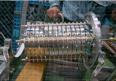
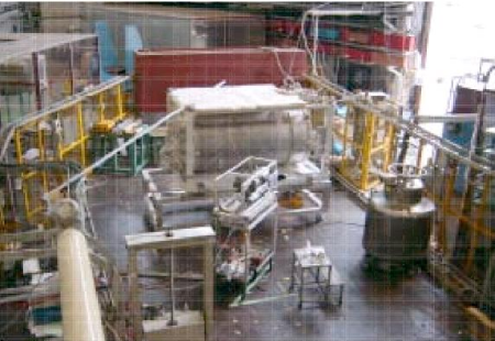
Figure 2.15: The MPT (left), used for measurements with cosmics in the DESY 5T magnet and in a test beam in a 1.2T magnet at KEK (right).

Gas Amplif. method	Gas	Pad Pitch( mm2)	Magnetic Field( T )
MWPC	TDR	2.3$\times$6.3	0, 1, 4(Cosmic)
GEM	TDR, P5	1.27$\times$6.3	0, 1
MicroMegas	Ar/C4H10	2.3$\times$6.3	0, 0.5, 1
w/ and w/o resistive foil

Table 2.7: Some of the parameters used for the MPT beam and cosmic ray tests.

Three different devices of gas amplification were tested with a combination of gas mixtures and read-out pad planes mounted in the MPT using a 4$GeV/c$ $\pi^{-}$ test beam; examples are listed in Table 2.7. The diffusion constant($C_{D}$) is a key parameter to determine a single-point resolution and was measured from using the behavior of signal-charge spread as a function of drift distance. The point resolution is naively parameterized by $\sigma_{r\phi}=\sqrt{\sigma_{0}^{2}+C_{D}^{2}/N_{eff}\times z}$, where, $\sigma_{0}$ is mainly determined by diffusion during gas amplification and by the ratio between signal-charge spread and geometrical pad size, $N_{eff}$ is the effective number of electrons contributing to the resolution as determined by effects of statistics, gain fluctuations and efficiency in amplification, and $z$ is the drift distance. The data obtained have been analyzed and compared with Monte Carlo simulation, preliminary results have been presented at recent conferences related to the ILC and the final results will be published in the near future.

Next R&D steps

As stated above, following tests using small prototype TPCs (Phase(1)), a Large Prototype (LP) TPC will be built and tested (Phase(2)). This will be carried out in conjunction with the EUDET program[22] for LC detector R&D. The LP work is expected to take the next four years and will be followed by Phase(3), the design of the LC TPC

Finally, to overview briefly the planning for the LC TPC and the LP, the tasks have been broken down into “Workpackages” as follows, and the tasks have been distributed among the LC TPC groups[30].

1. Workpackage Mechanics

   1. LP design (including endplate structure)

   2. Field cage, laser, gas

   3. GEM panels for endplate

   4. Micromegas panels for endplate

   5. Pixel panels for endplate

   6. Resistive foil for endplate

2. Workpackage Electronics

   1. ”Standard” RO/DAQ sytem for LP

   2. CMOS RO electronics

   3. Electronics, power switching, cooling for LC TPC

3. Workpackage Software

   1. LP software + simulation/reconstruction framework

   2. TPC simulation, backgrounds

   3. Full detector simulation/performance

4. Workpackage on Calibration

   1. Field map for the LP

   2. Alignment

   3. Distortion correction

   4. Radiation hardness of materials

   5. Gas/HV/Infrastructure for the LP

2.4 Calorimeter

2.4.1 Introduction

The final state in the next generation electron positron collider, ILC, will be dominated by the jets. At the high energy collisions, collimated multi-jets will emerge as the final states of quark, gluon and weak bosons. As we search for fundamental particles and interactions, the intrinsic interactions must be clarified from the final jets environment. The aim of the detector is to identify and separate the source of each jet. The collimated jet makes the detector configuration difficult to separate the particles in a jet, so that fine granularity is required. The information of jet-particle interactions in the calorimeter will help to resolve a jet. Not only the transverse granularity but also the longitudinal fine segmentation is indispensable. The larger the detector, the easier to resolve jet-particles. Thus the large detector makes the things simpler with less probability of overlapping of particle clusters. In order to resolve jet, the most important detector is the calorimeter by using PFA. With the help of PFA, one can analyze the jet components by ECAL for gamma contents and by HCAL for neutral hadron contents. The precision of jet energy determination is one of the measure of the calorimeter. The jet energy resolution is expressed as a sum of charged , gamma and neutral-hadron components.

$$\sigma_{j}^{2}=\sum\sigma_{c}^{2}+\sum\sigma_{\gamma}^{2}+\sum\sigma_{nh}^{2},$$

where $\sigma_{j}$, $\sigma_{\gamma}$, $\sigma_{nh}$ denote the energy resolution for a jet, a charged particle, a photon and a neutral hadron, respectively. The energy resolution for photon and neutral hadron are supposed to be scaled with $1/\sqrt{E}$. Thus these two equations hold.

$$\frac{\sigma_{\gamma}}{E_{\gamma}}=\frac{a_{\gamma}}{\sqrt{E_{\gamma}}}\ \ {\rm and}\ \ \frac{\sigma_{nh}}{E_{nh}}=\frac{a_{nh}}{\sqrt{E_{nh}}},$$

where two parameters are independent of energy, $a_{\gamma}=0.15$ and $a_{nh}=0.5$. The momentum resolution of tracker is expressed as

$$\frac{\sigma_{c}}{p_{T}}=5\times 10^{-5}p_{T}.$$

In Figure 2.16, these three resolutions are compared as a function of momentum or energy. At the lower momentum region, resolution for charged particle by tracker is much smaller than that for photons and neutral hadrons by calorimeter. Thus we can neglect the contribution from the charged particles in the resolution. Here the momentum resolution assumed is $0.4\times 10^{-5}p_{t}\oplus 0.8\times 10^{-3}$ (adding in quadrature) in red line, the energy resolution of ECAL is assumed to be $15\%/\sqrt{E}$ in blue line, and for HCAL, $50\%/\sqrt{(}E)$ in green line.

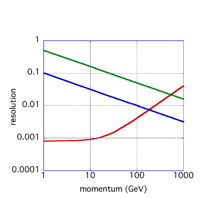
Figure 2.16: Resolutions as a function of pt or Energy. The red line shows for Tracker of $\sigma_{P_{t}}/P_{t}=1\times 10^{-4}p_{t}$, the blue line is for ECAL of $15\%/\sqrt{E}$ and the green line is for HCAL of $50\%\sqrt{E}$.

The square of jet energy resolution is expressed as

$$\frac{\sigma_{j}^{2}}{E_{J}^{2}}=\frac{a_{\gamma}^{2}\sum E_{\gamma}+a_{nh}^{2}\sum E_{nh}}{E_{j}^{2}}$$

The average photonic energy in jet is 25 % and that for neutral hadron energy is 10 %.

$$\frac{\sum E_{\gamma}}{E_{j}}\sim 0.25\ \ {\rm and}\ \ \frac{\sum E_{nh}}{E_{J}}\sim 0.10.$$

Finally,

$$\frac{\sigma_{j}}{E_{J}} = \frac{\sqrt{0.25a_{\gamma}^{2}+0.1a_{nh}^{2}}}{\sqrt{E_{j}}}$$

$$= \frac{\sqrt{0.056_{(\gamma)}+0.25_{(nh)}}}{\sqrt{E_{j}}}$$

$$= \frac{0.175}{\sqrt{E_{j}}}.$$

The ideal jet energy resolution is about 17.5 %. It is shown that the jet energy resolution is dominated by the energy resolution of neutral hadrons, although the average energy of neutral hadron is as small as 10 % in a jet. There is another more important factor to deteriorate the jet energy resolution. That is the shower overlapping of multi-particle jet. As the energy of jet is bigger, the overlapping effect becomes more serious. The overlapping effect might be reduced by optimizing the detector segmentation and layer. It should be clarified by hadron simulation, however, there are no reliable simulator. We have to make a prototype to test these simulators. There is an effect of neutron which will give delayed signal after the jet production, due to the slow neutron generated from hadronic interaction in the HCAL. The neutron may carry some part of jet energy. In order to measure the neutron contribution in jets , we need proton rich active material to be sensitive against the neutrons.

ECAL is used to measure photons precisely. HCAL is placed behind ECAL to measure neutral hadrons. In order to obtain the high jet energy resolution by PFA, both ECAL and HCAL need to have finer granularity than those employed for recent experiments such as LEP and LHC. The photon shower in ECAL and neutral hadron shower in HCAL should be separated and distinguished from neighboring charged particles. The shower clustering algorithms and fine granularity are crucial to realize this performance. However, developments of algorithms are in progress, and the granularities of calorimeters are yet to be optimized.

The average distance of two photons from $\pi^{0}$ decay is plotted as a function of incident momentum for GLD ECAL in Fig 2.17. It is shown that at least the size of the minimum detector cell is smaller than 1 cm up to 50 GeV $\pi^{0}$. On the other hand, neutral hadron clustering is difficult, since it would contain some hadrons whose interaction length is much longer than radiation length for electromagnetic shower case. The cluster size of HCAL becomes bigger than the ECAL. This indicates rather bigger segmentation allowed for HCAL, as far as the algorithms works fine with respect to ECAL case.

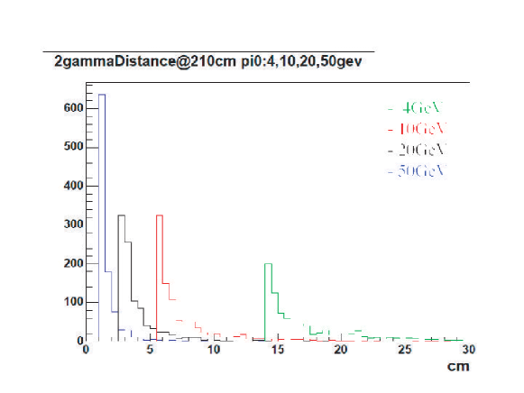
Figure 2.17: $\pi^{0}$s with certain momentum are generated and decayed into two photons that are measured at the front surface of ECAL ($R=210$ cm) with their distances. This distance is in the horizontal axis. The incident $\pi^{0}$ momentum are 4, 10, 20 and 50 GeV. It is found that the $\pi^{0}$ of 50 GeV or less energy can be detected separately with the granularity of 1 cm by 1 cm.

2.4.2 Electromagnetic calorimeter

Baseline design

In order to optimize the GLD detector concept for the Particle Flow Algorithm (PFA), the electromagnetic (EM) calorimeter is required to have:

• Large inner radius to separate particles with each other,

• Small effective Moliere radius to resolve near-by EM showers, and

• Fine granularity both in transverse and longitudinal directions.

We propose a tungsten-scintillator sandwich calorimeter to fulfill these requirements. Tungsten is chosen as the absorption material because of its small Moliere radius (9 mm). Scintillator is chosen as the active detector material. The scintillator is read out by the tile/fiber technique first used for the CDF plug upgrade EM calorimeter. The tile/fiber system has the following features:

• Essentially crack-less hermeticity,

• Capability for very fine longitudinal segmentation,

• Capability for fine transverse segmentation, and

• Less expensive than silicon pads.

The last item is important to realize a very large EM calorimeter. A layer of the EM calorimeter has a 3 mm thick tungsten layer, a 2 mm thick scintillator layer, and a 1 mm thick space for services, resulting in one-layer thickness of 6 mm and an effective Moliere radius of 18 mm. Both barrel and endcaps of the EM calorimeter have 30 such layers, corresponding to a total thickness of $26X_{0}$.

We have two options to realize fine transverse segmentation.

1. Strip array: This is the baseline configuration where a scintillator layer is composed of short strips. A super-layer is schematically shown in Figure 2.18, where two tungsten layers and two scintillator layers ($X$- and $Y$-layers) make a super-layer. The scintillator strips in $X$- and $Y$-layers are arranged to orthogonal with each other. The width of the strips is 1 cm, about a half of the effective Moliere radius of the EM calorimeter. This strip array is expected to have an effective granularity of 1 cm $\times$ 1 cm. To suppress ghost images which may appear when multi-particles hit a small area of the strip array, strips should not be long. The strip length is tentatively 4 cm and will be optimized by simulation studies.

2. Small tiles: This is a backup solution. A scintillator layer is composed of small square tiles. This configuration is free from the ghost image problem but has less granularity than the strip-array configuration. The tile size is tentatively 2 cm $\times$ 2 cm, and will be optimized by simulation studies.

The number of the scintillator strips/tiles amounts to about 10 millions. To keep the fine granularity, signals of all the strips (tiles) must be individually read out. Photons from each scintillator strip (tile) are read out via a WLS fiber embedded in its straight groove. A very compact photon detector such as SiPM/MPPC is directly attached to the WLS fiber at the end of the strip. The photon detector has a high gain ($\sim 10^{6}$) with no pre-amplifier. The electric signals of the photon detectors are then transported with thin flex cables to the calorimeter end where the signals are digitized. To keep the cost of the EM calorimeter reasonable, the photon detectors and readout electronics must be cost-effective.

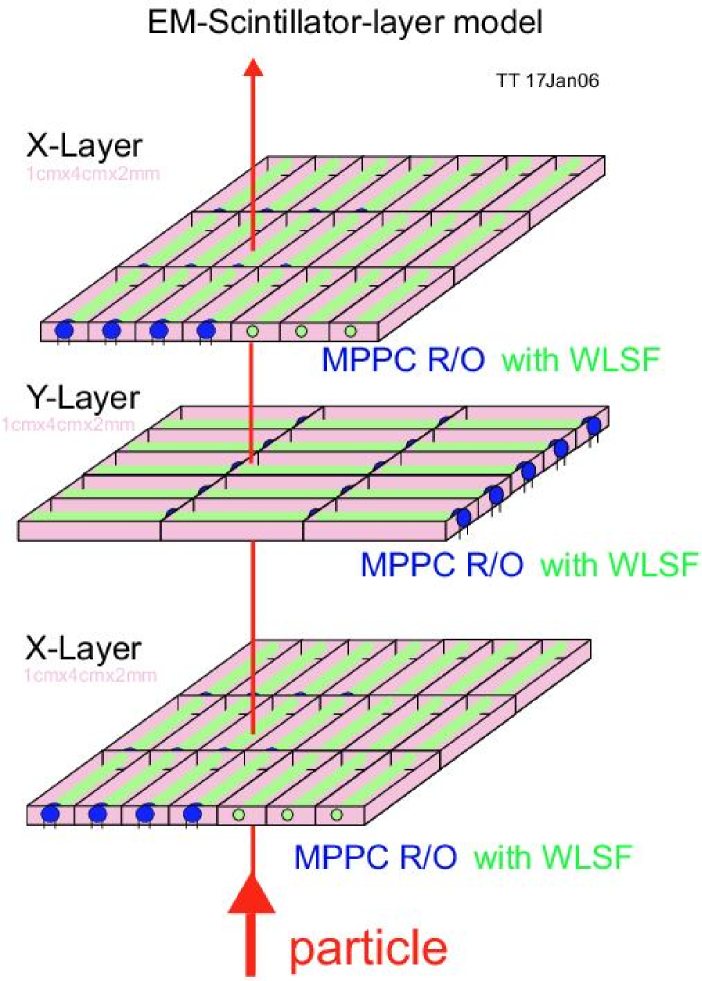
Figure 2.18: Schematic view of a super-layer of the strip array EM calorimeter.

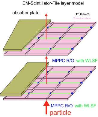
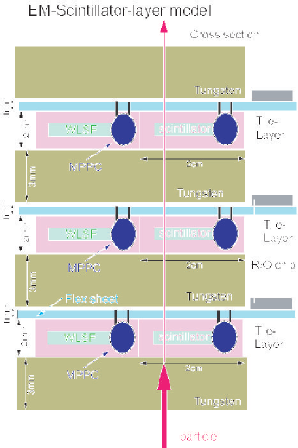
Figure 2.19: Schematic view of the layout of the small-tile EM calorimeter.

The parameters of the EM calorimeter are listed in Table 2.8.

Table 2.8: Parameters of the EM calorimeter.

Barrel Inner Radius	210 cm
Barrel Outer Radius	228 cm
Endcap Inner Radius	40 cm
Endcap Face Z-location	280 cm
Angular Coverage
Full thickness	$|\cos\theta|\leq 0.990$
Partial thickness	$|\cos\theta|\leq 0.991$
Thickness
Single layer	$0.86X_{0}$
30 layers	$26X_{0}$
Transverse segmentation
Strip-array option	1 cm $\times$ 4 cm (tentative)
Small-tile option	2 cm $\times$ 2 cm (tentative)

2.4.3 R&D studies

Test beam results of strip-array ECAL

An EM calorimeter test module, made of scintillator strips and lead plates, was constructed and tested with beam at KEK-PS  [36]. The purpose of the test beam was to study EM shower development extensively as well as to evaluate the performance of the energy, position and angle measurements for incident electrons.

The test module (Figure 2.20) consisted of 24 sampling layers, each of which had a lead plate (4 mm thick) and two scintillator layers (2 mm thick each) with a cross section of 20 cm $\times$ 20 cm. In each scintillator layer, twenty strips (1 cm $\times$ 20 cm) were laid out so as to make the two neighboring layers orthogonal ($X$ and $Y$). Signal was read out with multi-anode PMTs per super-layer which was defined as four successive $X$- or $Y$-layers. In the beam test, a tracking system was placed upstream of the calorimeter in order to reconstruct a track of the incident particle.

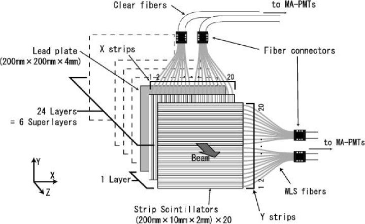
Figure 2.20: Schematic view of the strip-array EM calorimeter module.

By using electron beam of energies from 1 to 4 GeV/c, performance of the calorimeter was evaluated. The energy resolution ($sigma_{E}/E$ ) was found to be $((13.10\pm 0.12)/\sqrt{E}\oplus(0.00^{+0.73}_{-0.00}))$ %, which was consistent with the Monte Carlo simulation. The position resolution for the $x$ coordinate ($\sigma_{X}$) at the second layer (around the shower maximum) was $((4.5\pm 0.0)/\sqrt{E}\oplus(0.0\pm 0.2))$ mm, For 4 GeV/c electrons, the $\sigma_{X}$ becomes 2.2 mm.

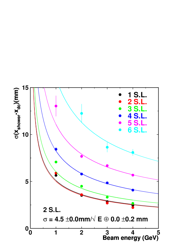
Figure 2.21: Position resolution as a function of the electron beam energy.

With the positions measured in the first four superlayers, incident angle of the electron beam was also measured. This measurement is important especially for detecting non-pointing photons. Obtained angular resolution ( $\sigma$ ) for 1 to 4 GeV/c electrons was $(4.8\pm 0.1)^{\circ}/\sqrt{E}\oplus(0.0\pm 0.5)^{\circ}$, and its linearity had no significant bias against the incident angle.

The response uniformity was examined by MIP signals and electrons. At the first superlayer, the response uniformity for the response summed over strips was measured, and the uniformity results were 2.4% for the shorter (1 cm-width) direction and 1.5% for the longer (20 cm-length) direction. With electron beams, the uniformity of the total energy measurement was found to be 1.1 %.

The lateral shower profiles were also studied in detail. We introduced $I(x)$, which was defined as the energy deposit integrated between minus infinity and $x$, divided by the total energy deposit:

$$I(x)=\int_{-\infty}^{x}\rho(x^{\prime})dx^{\prime}\bigg{/}\int_{-\infty}^{\infty}\rho(x^{\prime})dx^{\prime}$$

where $\rho$ represents the shower density. The origin of $x$ was set, event by event, to the particle incident position determined by the extrapolation of the reconstructed track.

Figure 2.22 shows the $I(x)$ distributions of each of the superlayers for 4 GeV/c electrons and that of the second superlayer for MIPs. The spread of the MIP signal mainly originated from light leakage between strips and cross-talks in the multi-anode PMT. On the other hand, the spreads for electrons mostly came from the EM shower spread in the calorimeter. Taking into account these detector effects, we can reproduce the spreads for the electron and also the expected effective Molière radius of 27 mm with the GEANT simulation.

Figure 2.22: Integral lateral shower profiles at each superlayer for 4 GeV/c electrons and at the second superlayer for MIPs.

Test beam results of small-tile ECAL

We performed the beam-test at the KEK in March 2004 and tested the prototype of the tile/fiber structure EM calorimeter.

Prototype module was a tile/fiber sampling-type EMCAL using 4 mm-thick lead absorber and 1 mm-thick plastic scintillator, total thickness is 17 $X_{0}$. Scintillator layer was separated by 4 cm $\times$ 4 cm tile size without the tile corner part to compose the mega-tile structure. WLS fiber was inserted in each tile groove and read out by MAPMT.

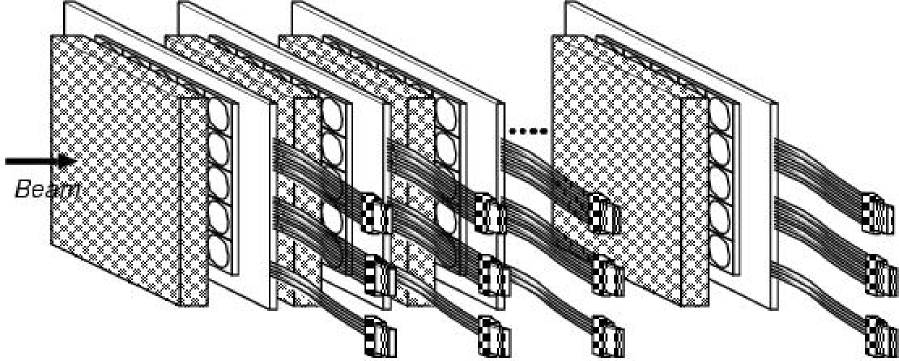
Figure 2.23: Front side view of the calorimeter module. Each layer was composed of alternately aligned lead sheet and scintillator

Energy resolution

We used 1 to 4  GeV/c electron beam for the energy resolution study. We achieved $16.0~{}\%/\sqrt{E}\oplus 3.5~{}\%$ energy resolution at center tile and the deviation from the linearity was less than 2.5%. Position resolution by reconstructing electron shower event was also checked and achieved $\sigma_{x}$ = 5.0 mm$/\sqrt{E}\oplus$ 4.9 mm.

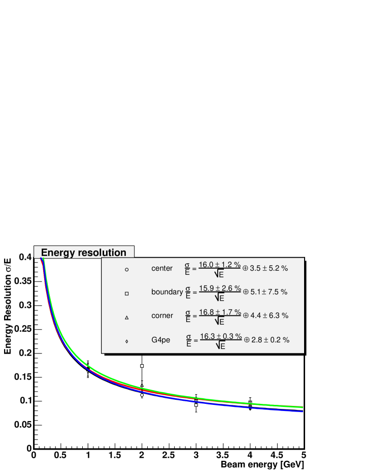
Figure 2.24: Energy resolution of each tile center($\bigcirc$), tiles boundary($\Box$), tile corner($\triangle$) electron incident events and the simulation results($\Diamond$).

Unifromity mapping

We tested the response uniformity by MIP like signals at the inside of the tile and boundary. Typical response uniformity at the center of tile was checked by 2 mm $\times$ 2 mm mesh size and good light containment was observed at the inside of the fiber groove. Also we checked responces to the MIP like signal in the central flat part ( -1.5 cm $\sim$ 1.5 cm ) along the x-axis and achieved $1.60~{}\%$ response uniformity in RMS.

Also we checked the response uniformity along the x-axis (-3 cm $\sim$ 3 cm) for electron signals integrated along the longitudinal direction with 4 mm $times$ 20 mm mesh size. We achieved 2.3% uniformity.

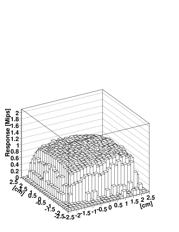
Figure 2.25: Response mapping by MIP like particles from one tile

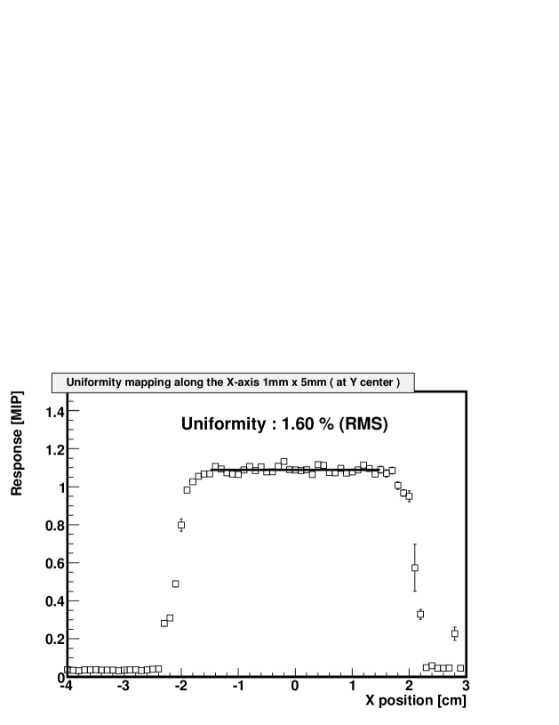
Figure 2.26: Uniformity mapping along the X-axis. The uniformity at the central region from -1.5 cm to 1.5 cm was 1.6%.

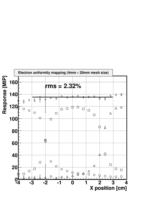
Figure 2.27: Electron mapping analysis along the x-axis. MIP signal was merged along the longitudinal direction and meshed 4 mm $\times$ 20mm(y). Uniformity achieved was 2.3% at the region of (-3cm $\to$ 3cm).

Absorber plates

As a test sample, a tungsten-alloy plate with a dimension of 200 mm $\times$ 200 mm $\times$ 3 mmt was produced by a Japanese company. Instead of pure tungsten, tungsten-alloy (W:Ni:Cu=95.0:3.4:1.6) was used for much easier manufacturing and handling. The density of the tungsten-alloy was 18.20 g/cm³ and the degree of hardness was 310 Hv. As the uniformity of the absorber material is important for good energy resolution, the thickness of the plate was measured at many points using a digital micrometer. The result is shown in Figure 2.28. The average, minimum, and maximum thickness was 3.016 mm, 3.006 mm, and 3.032 mm, respectively, and the RMS was 0.007 mm (0.23 %). If the uniformity of the thickness can be kept at this level, the effect to the energy resolution should be negligible.

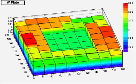
Figure 2.28: Thickness of the tungsten-alloy plate measured by a digital micrometer. The measurement could not be made at the middle part of the plate

Scintillator strips/tiles

Small plastic scintillators of different sizes, thickness and wrapping reflectors are systematically studied. A 16-channel photomultiplier tube (PMT) is used as read out through the 1.0 mm and 1.6 mm diameter wavelength shifting (WLS) fiber. The scintillating light generated by particles from the collimated ⁹⁰Sr source is collected from the scintillator by the WLS fiber and converted into electrical signals at the PMT. The best light yield scintillator is determined by comparing the measured pulse height of each 10$\times$40$\times$2 mm² strip scintillator covered with 3M reflective mirror film, teflon, white paint, black sheet, gold sputtering, aluminum evaporation and white paint+teflon. The position, length and thickness dependence of the 3M reflective mirror film and teflon wrapped strip scintillators are measured. The number of photons being emitted by the scintillator is also determined. As shown in Figure 2.29 the 3M radiant mirror film-wrapped scintillator has the greatest light yield with an average of 9.2 photoelectrons. It is observed that light yield slightly increases with scintillator’s length, but increases to about 100 % when WLS fiber diameter is increased from 1.0 mm to 1.6 mm.

Position dependence of the pulse height of the 10$\times$40$\times$2 mm³ scintillator strip wrapped with 3M radiant mirror film was measured. Figure 2.30 shows no significant change in pulse height along the scintillator strip. This means that there is uniformity of the light transmission from the sensor to the PMT along the scintillator strip. Figure 2.31 reveals the position dependence on pulse height across the strip scintillator. A dip is observed across the strip which is 40 % of the maximum pulse height that corresponds to the scintillator s thickness (300 $\mu$m) just below the 1.6 mm fiber. Small peaks are noticeable near the fiber with 1.6 mm WLS fiber.

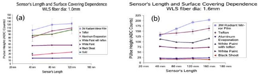
Figure 2.29: Strip length and surface covering dependence on pulse height through (a) 1.0 mm diameter WLS fiber and (b) 1.6 mm diameter fiber.

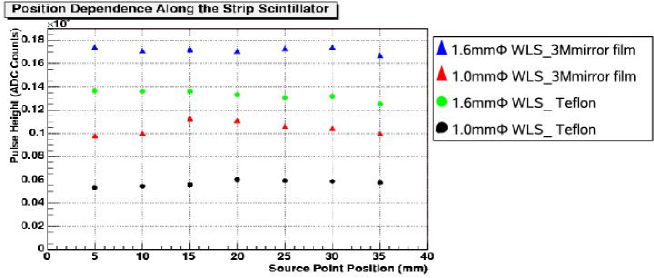
Figure 2.30: Position dependence of pulse height along the 10$\times$40$\times$2 mm³ strip 3M radiant mirror film wrapped scintillator.

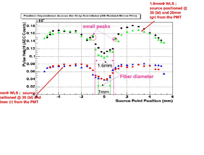
Figure 2.31: Position dependence of pulse height across the 10$\times$40$\times$2 mm³ strip 3M radiant mirror film wrapped scintillator.

Photon sensors

As the whole calorimeter is designed to be located inside the superconducting solenoid, photon detectors should be operational in strong magnetic field. In the case of crystal calorimeter, the light yield is large and popular PIN silicon photo diode or APD can be used. However, in the case of sampling calorimeter, the light yield is relatively poor and high-gain high-sensitivity photon detectors are needed. The photon detectors must also be very compact to be used for the fine-segmented calorimeter.

A new silicon photon detector, Silicon Photomultiplier (SiPM), has been developed by several Russian Groups. SiPM consists of many micro APD pixels being operated in limited Geiger mode, and the output signal is a sum of the signals from pixels fired by photons. A schematic view of the structure is shown in Figure 2.32.

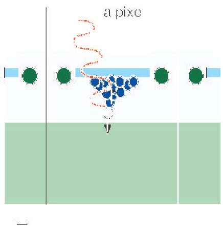
Figure 2.32: Schematic view of SiPM/MPPC structure.

A similar photon detector is also being developed with a name of Multi-pixel Photon Counter (MPPC) by Hamamatsu Photonics. Evaluations of some samples are in progress: SiPMs with 1156 pixels and MPPCs with 100, 400 and 1600 pixels.

The new silicon photon detectors are potentially ideal for tile/fiber readout because of the following characteristics.

• The silicon photon detectors are insensitive to magnetic field at all.

• They are very compact ($100\sim 1000$ pixels/1 mm²) and can be directly attached to the WLS fiber at the end of the scintillator strip (tile). No clear fibers are needed to transport the scintillation light to the photon detector.

• They have high gain ($\sim 10^{6}$) at bias voltage of $25\sim 80$ V. High gain amplification is not necessary in readout electronics.

• They have photon counting capability, good at measurement of low intensity light. The photon counting capability of an MPPC with 1600 pixels is demonstrated in Figure 2.33

  

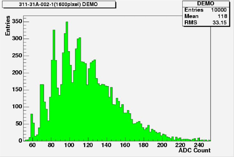
  Figure 2.33: Pulse height distribution of an MPPC with 1600 pixels with LED light.

• The signal output is fast enough for the timing measurement. A time resolution of 30 ps is obtained for 10 photoelectrons with a SiPM.

• The thermal noise rate of one photo-electron (one pixel) equivalent signal is rather high, typically about 1 MHz. This is not a serious problem because the bunch crossing timing is exactly known at the collider and a narrow gate can be used for charge integration.

However, SiPM/MPPC is a new and developing photon detector and there are many R&D items to be performed.

• According to a result of a test bench measurement where a 2 mm-thick scintillator strip, a 1 mm$\phi$ WLS fiber, and a conventional PMT ($QE\sim 20$ %) were used, the average number of photoelectrons was 2.5. To have more photon statistics, we will use 1.5 mm$\phi$ diameter WLS fibers. Therefore SiPM/MPPC with larger size to fit to the fiber diameter should be developed.

• Photon detection efficiency ($PDE$) of SiPM/MPPC is defined by the following formula:

  $$PDE=\epsilon_{geom}\times{QE}\times\epsilon_{G},$$

  where $\epsilon_{geom}$ is the geometrical efficiency (a fraction of active pixel area to the total device area), ${QE}$ is the wavelength-dependent quantum efficiency, and $\epsilon_{G}$ is the probability for a carrier created in active pixel area to initiate a Geiger-mode discharge. The photon detection efficiency of the existing SiPM/MPPC is typically 20%. Higher $PDE\sim 50$ % is desired to have more photon statistics.

• Dynamic range of SiPM/MPPC is limited by the total number of pixels in the device, $N_{tot}$. Neglecting cross talk effects, the relation of the output signal (the number of fired pixels, $N_{pix}$) and the number of photoelectrons, $N_{pe}$, is expressed as follows:

  $$N_{pix}=N_{tot}\exp(-N_{pe}/N_{tot}).$$

  For hadronic calorimeter and muon detector, $N_{tot}\sim 1000$ may be sufficient. For the EM calorimeter where electromagnetic showers make dense energy deposit in localized region, much more pixels is needed. According to a Monte Carlo simulation, at least $N_{tot}\sim 5000$ is necessary for the EM calorimeter not to degrade the energy resolution.

We measure the basic properties such as

• Gain and linearity,

• Noise rate

• Photon detection efficiency and

• Cross talks.

They are dependent on bias voltage and temperature.

To understand the performance of SiPM/MPPC, it is also important to measure

• pixel-to-pixel difference and

• position-dependent behavior in a pixel.

We perform such measurements with a YAG laser system in Niigata university, where the minimum spot size and the position precision of the laser beam are 2 $\mu$m and 2 $\mu$m, respectively. An improved test bench with a new laser system is being built at KEK dedicated to the measurements.

Some other properties are still to be tested.

• Long term stability,

• Radiation damage.

We need more samples to do the tests.

We feed back our test results to the companies for further improvements. Good communication between experimental groups and companies is essential.

Electronics

The calorimeter signals are sent from the photon detectors to the the front-end electronics through thin cables. As the gain of the new silicon photon sensor is high enough, we do not need any preamplifier. The output signal is so fast that the timing measurement can be performed with a good accuracy. An important thing is that there are huge (several ten million) channels, thus low power consumption and small dimension are very desirable.

The readout electronics should digitize an amplitude/current and timing information of the signal. The timing measurement is necessary to identify the bunch crossing, and the required resolution of about 10 ns can be obtained without difficulty. The about 1 ns time resolution will be required if we want to distinguish the energy deposits of slow neutrons. Moreover, with such accurate time resolution one may identify cosmic-ray muons. The time resolution of the optical system is dominated by that of the wavelength shifting fibers, but it is still possible to achieve it with the appropriate electronics.

The digitization will be done by either analog-to-digital converter (ADC) with a time-stamping capability or FADC. The dynamic range for the energy measurement is limited by number of cells in the photon sensor and the electronics. Note that the former has a saturation effect even below the overflow. In order to discriminate between a MIP and sensor noises clearly, A MIP signal should produce at least 10 hit cells at the photon sensor. On the other hand, the pulse height at the shower maximum is expected to be around 200 times that of the MIP signal. Therefore, the number of cells should be more than 2000, and the ADC or FADC is required to have 10-bit or more accuracy.

Another important role of the electronics system is to supply power to the silicon photon detectors. The device has very narrow range of the bias voltage for the operations ($<$ 1 V), thus the power supply should be very stable. In addition, the operational voltage range differs between pieces; it is more than a few V or 10 V in some cases. A possible solution would be to group the photon sensors such that the voltage range in a group can be small enough to be adjusted by, e.g. a digital-to-analog (DAC) converter within 5 V.

The power supply as well as the ADC or FADC will be implemented in an ASIC, which can have a buffer for storing data during a bunch train and a gigabit Ethernet to send data to the trigger/DAQ system. Some components for the ASIC exists, and the integration for all features are under development.

2.4.4 Hadron calorimeter

Baseline design

Global structure of the GLD calorimeter detector is shown in Figure 2.34.

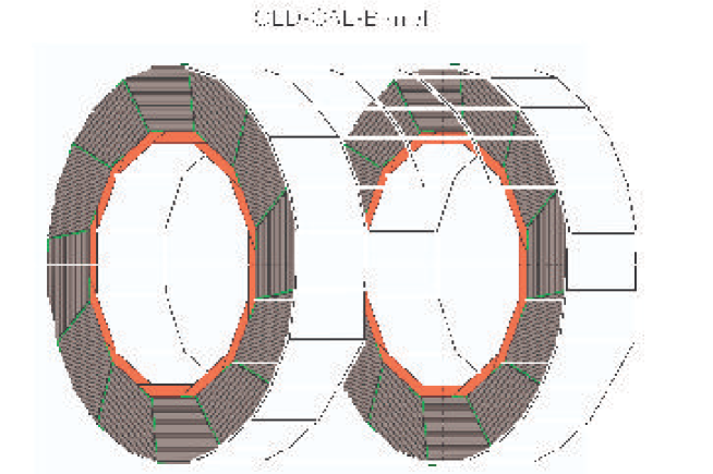
Figure 2.34: Schematic view the GLD barrel calorimeter.

The GLD hadron calorimeter consists of absorber (lead plate) and plastic scintillator sandwich. The plastic scintillator has a shape of strip, which has a straight gloove where a wave length shifting fiber (WLSF) is embedded. This readout scheme gives freedom for the strip length and width, since the pulse height from the WLSF does not depend on the position where a particle is passing by. As we are still trying to optimizing the strip length via simulation, we set the strip length to be 20 cm as the starting point. The width of the strip is set to be 1 cm, similar to the ECAL case, in order to achieve effective granularity of 1 cm $\times$ 1 cm with orthogonal strip layers (Figure 2.35). .

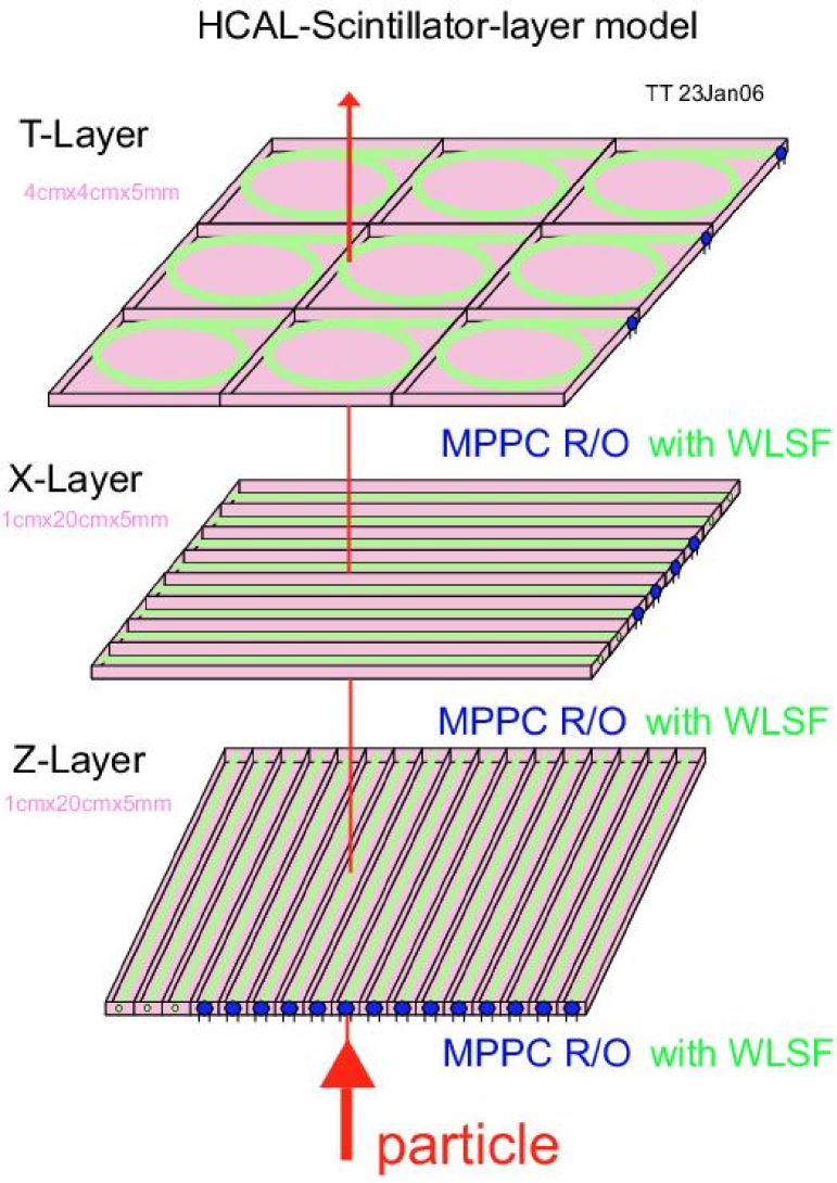
Figure 2.35: Schematic view of GLD-HCAL super-layer is shown. It consists of three layers of scintillator and lead.

The thickness of the scintillator is determined to have enough light output from minimum ionizing particles by newly developed photon sensors which has a pixel structure. As the base line design, the thickness is set to be 5 mm.

Lead is selected as the absorber material so as to achieve hardware compensation with scintillator. Since the energy resolution is governed by fluctuation of electromagnetic shower to the purely hadronic interaction, in order to minimize its fluctuation, electromagnetic shower output should be suppressed. According to our test beam results, the hardware compensation is achieved by adopting the ratio of lead : plastic scintillator = 9.1 : 2.

Choice of active material

Plastic scintillator is reliable and stable material for the particle detection. For a long time the plastic scintillator has been used to detect and measure not only the charged particles but also neutrons. One of the reasons to choose the plastic scintillator as the active media of the calorimeter sites on its reliability. Since we need fine granularity as ever constructed before, we have to be careful for the uniform response of each sub component in numerous number of pieces. The plastic scintillator is one of the candidates to satisfy this requirement, since the strip structure has flexibility for its size by using a wave length shifting fiber as scintillation light read out. A problem might be an increase of number of channels of photon detector for the read out system. Recent development of new type silicon photon sensor is quite promising for our detector. The progress is already discussed in the ECAL section. The light signal of scintillator is fast enough to measure the timings, with which we are able to reject background hits and to recognize neutron hits in the calorimeter.

The active material which contains hydrogen is sensitive to neutrons. It is important to detect and measure neutrons not only for the compensation but also for the total energy measurement of hadrons. Those neutrons appear at the tail of the hadron shower process from decays of excited nuclei.

Generations of their signals usually delays from a particle injection to the calorimeter. In simulation program used for evaluations of calorimeter performance, the nuclear excitation and its decays has to be taken into account properly.

Being equipped with the the read out electronics of time measurement capability, we are able to recognize the neutron signal from other charged hadrons. It is studied by a simulation base on Geant4.6.2. In the simulation, single-pions is injected into a test HCAL detector which consists of lead and plastic sandwich calorimeter of 100 layers. The thickness of the lead plates is 8 mm and that of scintillators is 2 mm, where the size of the detector is 1 m³. A typical shower eventinduced by a pion is shown in Figure 2.36.

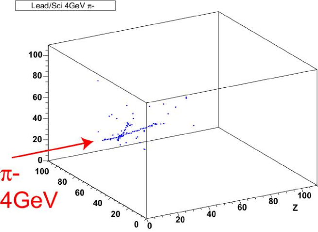
Figure 2.36: An event induced by a pion of 4 GeV into model HCAL of 100 layers. The thickness of lead is 8mm and that of scintillator is 2 mm with 1 cm by 1 cm cells of 1 M pieces. Axis labels are in unit of cm.

The hits are recorded in 1 cm $\times$ 1 cm cell of plastic scintillator of 2 mm thickness, when the energy deposit exceeds 10% of that of minimum ionization particles (MIPs). In the figure, satellite hits can be seen apart from the incident pion trajectory.

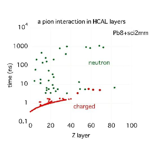
Figure 2.37: Timing information (vertical) is ploted as a function of layer numbers. The injected pion and its charged daughter hits are shown by red points, where the neutron contribution is shown by green points.

For the event shown in Figure 2.36, hit timing of each cell are shown as a function of layer numbers in Figure 2.37. In the figure, some charged components come from electrons and positrons produced by gammas in delayed decay of excited nucleus. These hits are also shown in red round marks in the figure. The figure shows a clear separation between neutron and charged components signals. According to this Geant 4 simulation, we can conclude that an inclusion or exclusion of neutron contribution in hadronic shower reconstruction are determined based on a timing information of hit cells.

The scintillator calorimeter can detect the neutrons effectively, while gas calorimeter can not. The energy measured by the scintillators are plotted as a function of timing cut in Figure 2.38. As seen in the figure, the energy deposit after 5 nsec amounts to about 20% of the total energy deposit. It can be attributed to the contribution of slow neutrons.

Figure 2.38: The otal energy deposited in the scintillators (red diamond) and the total number of hits (green bullet) are plotted as a function of timing cut. At 1000 ns, the energy shows without any time cut. This shows about 20% of energy is taken by slow neutrons.

On the other hand, the energy resolution becomes worse if we cut the slow components of signal at 5 nsec as seen in Figure 2.39.

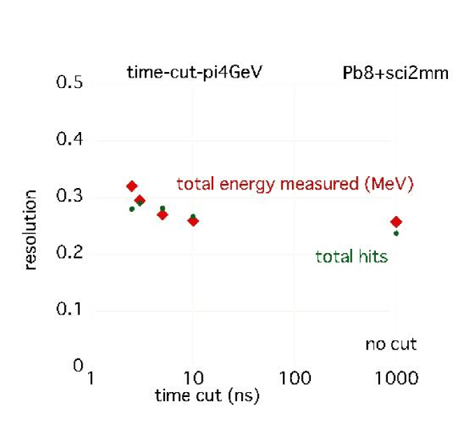
Figure 2.39: The energy resolution of HCAL(red diamond) and the total number of hits (green bullet) are plotted as a function of timing cut. The point at 1000ns means without any time cut applied. This figure shows the energy resoluion becomes worse about 20% if 5 nsec timing cut is applied to take out slow neutron components.

The spread of hadron shower with and without the timing cut of 5 nsec is shown in Figure 2.40 (a) and (c). For comparison, similar plots in the case of iron-absorber calorimeter are shown in Figure 2.40 (b) and (d), where the thickness of the iron absorber and scintillator is 20 mm and 5 mm, respectively. Thicker material thickness is adopted to simulate with a configuration similar to the calorimeter baseline desing. Since the nuclear interaction lengths of iron and lead are similar, the ratio of absorber and sensor thickness are same for the both cases.

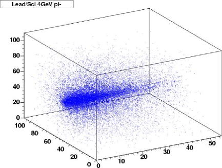
(a)	(b)
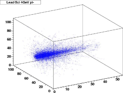
(c)	(d)

Figure 2.40: The event displays with 1000 events of 4 GeV/c pions overlapped are shown. Labels on axes are in unit of cm. The upper left figure (a) and the upper right figure (b) is for the case of lead absorber and iron absorber, respectively, without the timing cut. The lower left figure (c) and the lower right figure (d) is for lead and iron absorber, respectively, with the timing cut of 5nsec. The neutron hits which scattered out from the interacting core region are more significant for lead absorber.

A thousand of pions are injected and events are overdrawn in a same figure. The outer shower cloud is due to the slow neutron component, whose spreads are determined by the nuclear interaction lengths of the absorbers. Since the nuclear interaction lengths of lead and iron are similar, the sizes of the outer shower clouds are similar. On the other hand, the size of the central part of shower in the lead absorber calorimeter is smaller than that of iron absorber calorimeter, because the radiation length of lead, which characterizes the size of the central part of shower, is much shorter than that of iron. This effect is more clearly seen when slow neutron components are cut off by applying a timing cut of 5 nsec in Figure 2.40.

This is more clearly shown in Figures 2.41 and 2.42. These figures show the averaged energy weighted radius of shower ($\bar{R_{E}}$) in lead and iron absorber calorimeter with (Figure 2.42) and without (Figure 2.41) cuts of 5 nsec timing. The $\bar{R_{E}}$ is defined as follows:

$$\bar{R_{E}}\equiv\sum_{i}{r_{i}e_{i}\over e_{i}}$$

where $r_{i}$ is a distance between the shower axis and a cell. $e_{i}$ is the energy deposit in the cell, and $i$ runs for all hits in the event. Figure 2.42 shows that the central part of shower in lead-based calorimeter is smaller than that of iron-based calorimeter.

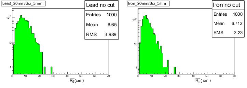
Figure 2.41: Averaged energy weighted radius of showers in lead(left) and iron(right) calorimeter, respectively. No cut on cell timing is applied.

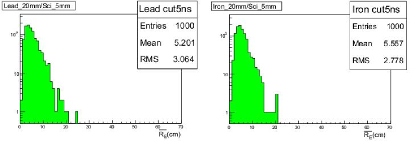
Figure 2.42: Averaged energy weighted radius of showers in lead(left) and iron(right) calorimeter, repectively. Hit timing of each cell is required to be within 5 nsec from particle incident to the calorimeter.

We used the strip shaped scintillator for the calorimeter readout to achieve the effective readout granularity of 1 cm $\times$ 1 cm. This is correct as far as a passage of charged particle in x and y strips is concerned. We are developing an algorithm to resolve the problem when multi-particles pass through in small area. When the analog information from a strip is available, we will be able to recognize two particles with their pulse heights.

Choice of absorber material

We have two candidates for the absorber materials of the HCAL. One is lead which has good nature to have compensation in reasonable dimensions, while the other is iron or steel whose compensation condition is not far from the reality. The compensation means the total measured energies with an HCAL by electrons and hadrons have same amount. With lead, the compensation condition is achieved at 9.1 mm lead vs 2 mm plastic scintillator thickness according to our test beam results [34]. The compensation condition for iron or steel is not found by experiments, however, R. Wigmans expects it to be Fe/scintillator to be 15/1 in the thickness, while his prediction for lead is Pb/scintillaotr to be 4/1. The compensation can not be achieved by Liquid Ar, since it does not contain hydrogen atoms. The crucial role of hydrogen in the active material has been demonstrated in L3 experiment at LEP.

Lead has shorter radiation length than that of iron, while the interaction lengths are similar. As discussed already and shown in Figures 2.40, 2.41, and 2.42, the lateral spread of shower in a calorimeter using lead absorber is smaller than that using iron absorber. The smaller lateral spread of shower is preferable for efficient particle flow analysis.

Here we discuss the calorimeter absorber from the detector point of view. In the engineering point of view, the iron absober is preferred because mechanical strength of iron is much higher than that of lead.

2.4.5 R&D studies

We have already studied the lead scintillator sandwich hadron calorimeter in the test beam. The results have been published elsewhere [35]. With 20 cm by 20 cm tile, we have constructed 1 m³ HCAL, which were segmented in 100 (= 5 x 5x 4) parts. The schematic view of the detector is shown in Figure 2.43.

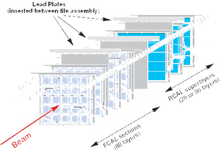
Figure 2.43: Schematic view of hadron calorimeter test module in 1999 at Fermilab

A tile of 2 mm thick plastic scintillator were used for the active material and 8 mm thick lead plates were the absorber in this HCAL. Wave length shifting fiber was embedded in a groove of a tile in order to read the scintillation light. The energy resolution measured up to 200 GeV was plotted for pions and electrons in Figure 2.44.

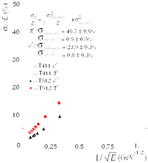
Figure 2.44: The energy resolutions for electrons (green triangle) and pions (red circle) as a function of incident energy.

The e/p ratio which is the measured energy ratio of electrons to pions is plotted in Figure 2.45.

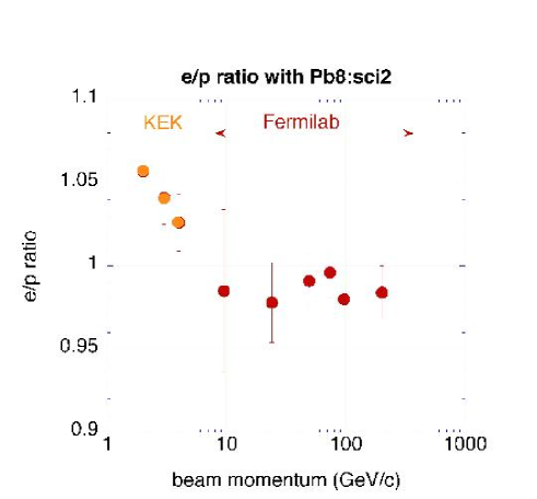
Figure 2.45: The e/pi ratios as a function of incident beam momentum. At high energy, it closes to 1.0.

Figure 2.45 shows the hardware compensation at higher energy region, since the e/p ratio is very close to be 1.0. At lower energy region, we have measured the e/p ratio [34] by changing the volume ratio of lead and plastic scintillator. The result is shown in Figure 2.46.

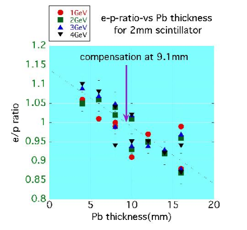
Figure 2.46: The e/pi ratios as a function of absorber (lead ) thickness in mm. The compensation condition is achieved at 9.1 mm of lead plate.

By fitting those data except 1 GeV data, we found that the compensation is achieved at 9.1 mm of lead thickness when the plastic scintillator is 2 mm thick. The expected value of lead thickness by R. Wigmans is 8 mm for 2 mm scintillator. The tile size was 20 by 20 cm² for those data. A schematic view of groove for WLFS is shown in green in Figure 2.47. The thickness of the plastic-scintillator is 2 mm, where we make groove of 1.2 mm to embed the WLSF of 1 mm.

With the size of 20 cm by 20 cm , we have experienced and tested the HCAL.

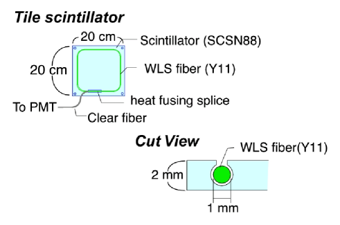
Figure 2.47: A tile scintillator and its cross section around the fiber groove.

2.4.6 calibration system

Unlike the gas chamber in the calorimeter, the stable response of the plastic scintillator is well known. However, we must have a system to monitor and calibrate the detector response. There are several ideas to check the response beside the test pulse into the electronics circuit to test the performance.

1. Calibration with cosmic muons Suppose the size of a strip is 1 cm x 20 cm , expected number of cosmic muons passing by is 0.1/cm²/min $\times$ 20 cm² = 2/min. This number is obtained assuming that the detector is located close to the ground. For the calibration, we need about 100 muons for each strip. This will be achieved only in 50 minutes.

2. Calibration on $Z^{0}$ pole Since the cross section of $Z^{0}$ pole is very high, there is an idea to operate the collider at the $Z^{0}$ pole to collect calibration particles, not only for HCAL but also for other detector components. Assuming an integrated luminosity of 1 fb^-1, we have 25 muons / strip. This number is not sufficient for calibration, however, the high energy 45 GeV muons are much more reliable than cosmic ray muons. We keep this method as an option for calibration.

3. Halo muons for the endcap HCAL calibration A large number of background muons are expected to be generated along the ILC beam line. The number of the halo muons are so large that the muons will be used for the calibration of HCAL in the endcap region, where the strips are orthogonal to the beam line.

Relative monitoring of scintillation strips is discussed in the next section.

2.4.7 Missing R&Ds

1. Relative calibration scheme We need to have a stable light source to calibrate each scintillator strip, otherwise we can’t follow the response of all strips. While the beam or cosmic ray calibration discussed above have limited statistics, the light source system to illuminate the strip has no such statistical problems. Systematic fluctuation of light source is rather problematic in this case. Here we have an idea to feed laser or LED light to many strips simultaneously with clear fibers (Figure 2.48). The problem is expected at the light connection between the fiber and each strip point. Here we have found a good solution to reduce the number of light source which will be the main source of the systematic errors.

   

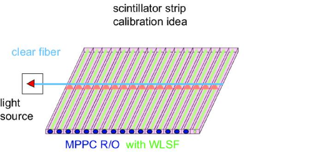
   Figure 2.48: Schematic view of relative calibration of strips by a clear fiber.

2. Support structure by engineering study Since we suppose to construct the HCAL with lead and scintillator sandwich, we have to take into account the mechanical structure of the lead plates. The pure lead plate is not stiff enough as the structure material, however, by adding Molybdenum , hardness increases and becomes stiff enough to support itself. For real structure of HCAL, we have to study this point furthermore.

3. Other options

   • Square tile not strip array scintillator

   • Iron instead of lead as absorber

2.5 Muon detector

2.5.1 Introduction

The main task of the muon detector is to identify muons. The muon momentum is precisely determined by the inner tracking devices, therefore the muon detector should measure hit positions with modest accuracy in order to associate them to the fitted track. However, an independent momentum measurement of the penetrating particle by the muon system would be preferable, especially for energetic or well-collimated jets, for better matching with the extrapolated track or even better identification of the secondary muons. Modest timing resolution is also required to tag cosmic-ray muons and to identify the bunch crossing as well as to reject backgrounds.

A secondary task of the muon detector is to measure the energy leakage of the hadron showers, i. e. work as the tail catcher. The total energy of particles entering the muon detector was estimated by a Geant4 simulation for the case of the process $e^{+}e^{-}\rightarrow b\bar{b}$ at 500 GeV center of mass energy and shown in Figure 2.49. As seen in the figure, about 10% of the total evern energy leaks into the muon detector. Since the jet energy resolution is expected to have 30%/$\sqrt{E}$ with the particle flow technique, the tail catching may become more important than the previous experiments.

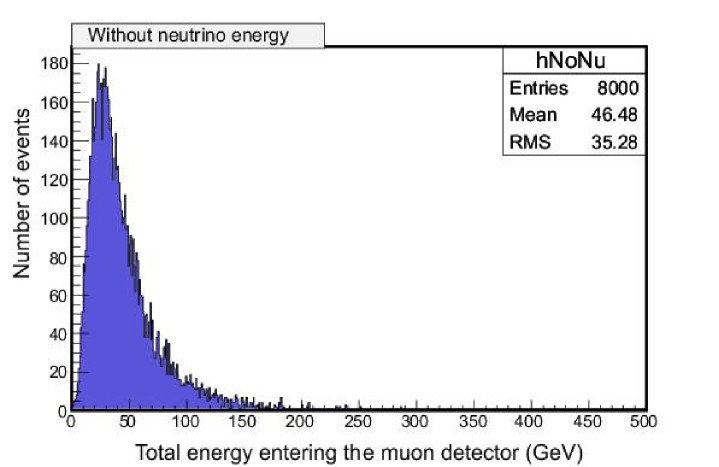
Figure 2.49: Total energy of particles entering the muon detector, except neutrino, in each event of $e^{+}e^{-}\rightarrow b\bar{b}$ at 500 GeV center of mass energy.

The muon detector will be located outside the hadron calorimeter and the solenoid coil. The muon identifiers are interleaved between the return yoke layers which function as absorbers in the muon system. The magnetic field strength is about 3 Tesla and the total iron thickness is about 2 m. The structure of the return yoke will be optimized for better field strength in both the bore and the fringe. On the other hand, the shape of the muon system, number of active layers, segmentations and detector technology will be chosen by evaluating the muon identification efficiency and the energy measurement efficiency by the Monte Carlo simulation and the hardware R & D’s.

Although detector occupancy is supposed to be relatively low in case of $e^{+}e^{-}$ collisions, we need to verify that the muon detector, especially in the forward region, can cope with dense jets or particles. Detector coverage and hermeticity of the muon detector should be excellent for the good detection efficiency and the measurements of the missing momentum with good accuracy.

The association of inner muon tracks with the segments of the muon detectors suffers from energy loss and multiple scattering in the calorimeter and the coil, and the return yoke itself. The muon momentum is required to be more than 3.5 GeV to go through the coil, and to be more than 6 GeV to fully penetrate the return yoke in the barrel region , as shown in Figure 2.50. Hence, in the low momentum region muons have to be identified by only the calorimeter, and just below 5 GeV the range measurement in the muon system would help the energy measurement of the particle.

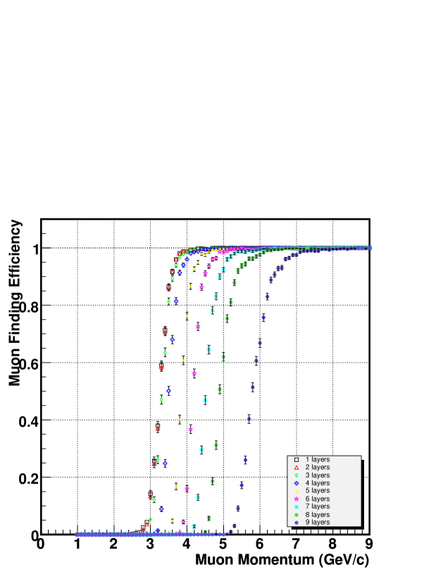
Figure 2.50: Muon detection efficiencies as a function of the muon energy in the baseline GLD configuration(see Figure 1.2). The results are obtained by using the Jupiter. The efficiency threshold is found to be 3.5 GeV requiring a hit in the first layer, or 6 GeV requiring hits in all layers.

The spatial resolution of the muon system needed for the track matching should be less than the spread from the multiple scatterings for muons, given that no other particles pass through nearby. The spatial spread for single muons is obtained by the full simulator, as shown in Figure 2.51. In the simulation, muons are generated at the interaction point and emit into the direction of cos $\theta$=0. The hit position is taken from the $z$-coordinate of the muon at the first active layer.

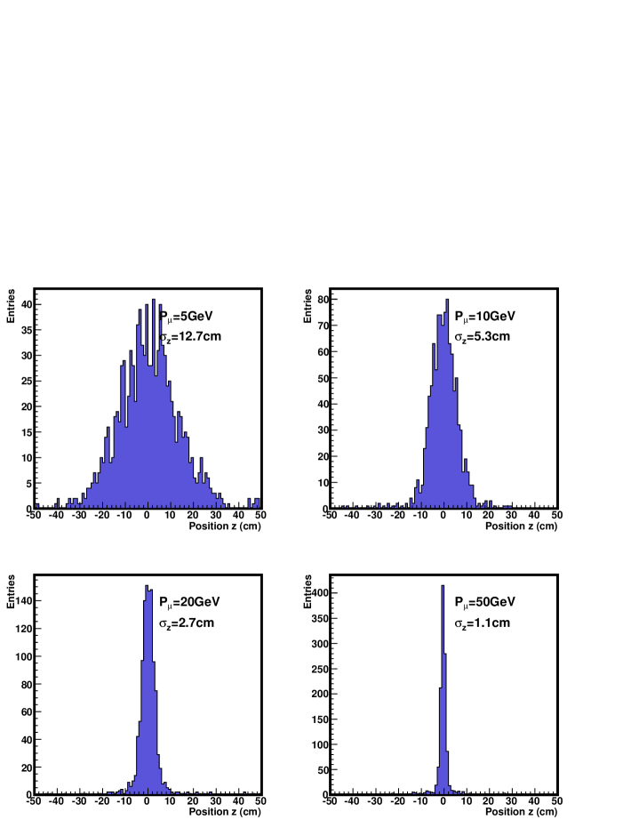
Figure 2.51: Distributions of the $z$-coordinate at the first layer for muons of $p_{\mu}$=5 GeV, 10 GeV, 20 GeV and 50 GeV.

The relevant muon momentum region is examined by events including jets, for example $e^{+}e^{-}\to b\bar{b}$ at $\sqrt{s}$ = 500 GeV (Figure 2.52). As seen in the histogram, the average momentum is 20 GeV/$c$ and the majority of the muons are below 50 GeV/$c$. As the result, we conclude that the position resolution of about 1 cm is sufficient for the good association of charged tracks from the inner trackers.

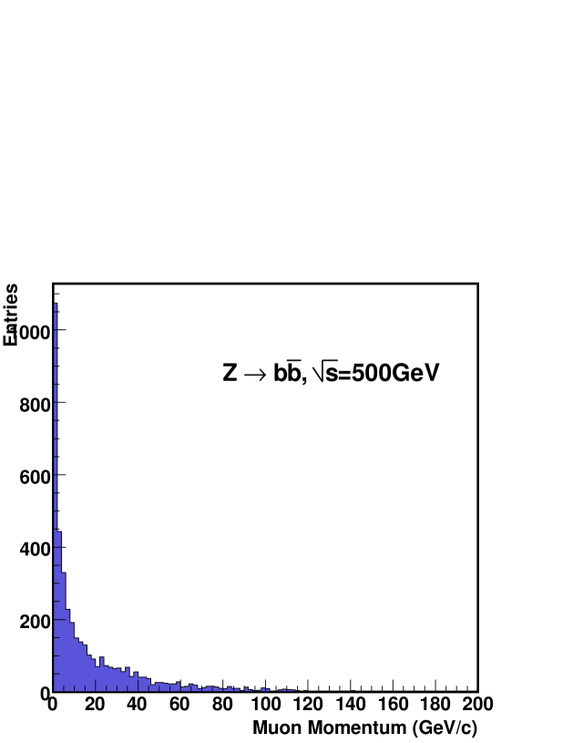
Figure 2.52: Muon momentum distribution at the front face of the muon detector for $e^{+}e^{-}\to b\bar{b}$ at $\sqrt{s}$ = 500 GeV.

2.5.2 Baseline design

In the GLD detector, the muon detector covers a very large region and is sandwiched between the return yoke. This implies that the technology should be inexpensive and reliable because it will be difficult to access and replace, and we have to operate it

for more than a decade. Also, the detector must be tolerant of

the radiation and the aging. Therefore a well-established technology must be chosen, and we adopt an scintillator-fiber technique as the

baseline design. Since this technology is also chosen for the

calorimeter, we will be able to save the cost for production

as well as R&D’s. Photon sensor will be a Geiger-mode photon

counter, which is being developed actively, can also be shared

with the calorimeter, and the read-out electronics is similar to

that of the calorimeter. Sensitivity to neutrons is also an issue for the scintillator, as discussed in the calorimeter section, and the timing information may be helpful again.

The cross-sectional view of the

muon detector is shown in Figure 1.2. It has an dodecagonal shape in the $r$-$\phi$ view. There are nine active layers in both barrel and endcap regions, and each active layer has two orthogonal layers of the scintillator-bar arrays. The scintillator bar has a cross section of 5 $\times$ 5 cm and the length varies according to the location. A wavelength shifting (WLS) fiber is embedded into the straight groove along the scintillator, and at the both ends of the groove the silicon photon sensors are directly attached to the fiber. The scintillator and the WLS fiber might be too long to propagate photons to the sensors, and we may need to break the scintillator into pieces to decrease the light attenuation. In this case we still keep the detection efficiency high to minimize the dead space. With the readout at both ends, we can obtain the rough hit position along the scintillator by the time difference of the signals.

Detector calibration will be performed by using cosmic muons for the barrel region and halo muons for endcap regions. Because the scintillator size is large, we can calibrate the system within a few % level. Additional calibration system (LED etc.) may be used for the backup.

2.5.3 R&D studies

Since the scintillator-fiber scheme is well-established, we concentrate on photon sensor for hardware R&D’s, and it is already described in the calorimeter section. The electronics for the muon detector is also almost the same as that for the calorimeter.

Simulation studies have been performed to investigate the following items: (1) hit density at the front of the muon detector, (2) hit point smearing due to the material in front of the muon detector and the return yoke.

2.5.4 Missing R&Ds

In order to finalize the detector design, some parameters are still to be optimized. They are number of layers, scintillator thickness and width. More simulation studies for the muon detection efficiency and the tail catching capability are needed for tuning those parameters.

For the hardware study, as the scintillator bar and the WLS fiber become very long, care should be taken for the optical quality of the detector so that the photon sensors can receive enough photons. Thus, the optical characteristics of the scintillator and the WLS fiber, scintillator length and photon-detection efficiency of the photon sensors should be tested and justified for real use.

Although the scintillator-fiber system is expected to perform well, another technology is considered as an option, which is resistive

plate chambers (RPCs). Large area RPC systems have been used by experiments at $B$-Factories. RPC has simple structure and can be built with inexpensive cost. However, RPC needs a mixture of gases which should be avoided if possible for stable operations.

2.6 Small Angle Detectors

2.6.1 Introduction

At linear colliders it is expected that a large number of $e^{+}e^{-}$ pairs are created by the QED process $\gamma\gamma$ $\rightarrow$ $e^{+}e^{-}$ where $\gamma$ may be off-shell or near-on-shell [37]. If the charge of the created and the on-coming bunch have the same sign, it is known [38] that distributions of $p_{T}$ and azimuthal angle of the created particles can be used to study $\sigma_{x}$ and $\sigma_{y}$ of the on-coming bunch. It should be noted that this technique allows to measure independently the size of the two beams because the created particles are deflected asymmetrically in the forward and backward angular regions if the two beams have different parameters. The goal of the pair monitor is to detect the $e^{+}e^{-}$ pairs in order to extract the beam profile parameters.

Also, at linear colliders it is expected that a precise measurement of the luminosity can be achieved by detecting electrons from Bhabha scattering. Calorimeters capable of detecting electrons at the very forward regions are typically used for such luminosity measurement. Another important role of such calorimeters is to veto forward leptons. It becomes important as it is closely related with the detection of sleptons [39], in the scenario where the lightest SUSY partile (LSP) is the lightest neutralino $\tilde{\chi_{1}^{0}}$.This particle is considered as the best candidate to satisfy the cosmological constraints on the dark matter in the universe. The WMAP [40] results imply a very small difference between the lightest slepton mass, the SUSY partner of the $\tau$ which will be called $\tilde{\tau}_{1}$, and the LSP mass. Since this feature is quite general, it is important to have an experimental access on the detection of sleptons at the future linear collider. Experimentally, one needs to measure $\tilde{\tau}_{1}$ decaying into a $\tau$ lepton with one or two neutrinos in the final state which even further reduced the amount of visible energy. Near threshold, the cross section is at the 10 $fb$ level with a potentially very large background due to the four fermion final states, the so-called $\gamma-\gamma$ background, which is at the $nb$ level. In usual cases the standard backgrounds can be eliminated by vetoing forward electrons. Therefore, another important role of calorimeter detectors at small angles is to veto background events by identifying electrons in the forward region.

In this document, we call small angle detectors as a set of the following detectors: forward calorimeter (FCAL), the beamline calorimeter (BCAL), and the pair monitor (PM). Silicon-Tungsten sampling calorimeter is the default technology for both FCAL and BCAL. As an option, diamond/W detector is considered since the diamond is the radiation hard sensor. FCAL can also serves as a beam mask. PM serves as a beam profile monitor. A 3-dimensional silicon pixel technology is chosen for the PM. In following sections, we discuss technology choice, configuration, and performance of each detectors.

2.6.2 Forward and Beamline Calorimeters

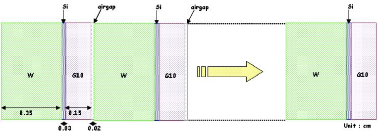
Figure 2.53: FCAL geometry

The FCAL is located behind the endcap of the TPC in $z$ direction. It is a cylindrical structure with its axis coinciding with the $z$ axis ( see Figure 1.3). It has 45 layers of Silicon-air gap-Tungsten sandwich. Thebaseline thickness of the detector is described in Table 2.9.

Table 2.9: Summary of parameters for the FCAL

Material	Thickness (cm)
Silicon	0.03
G10	0.15
Air	0.02
Tungsten	0.35

The geometry of the FCAL is described in Figure 2.53. One sandwich is 5.5 mm thick and in total thickness of the FCAL becomes 250 mm. The FCAL covers from 260 cm to 285 cm in $z$ coordinates and from 12 cm to 36 cm in the radial coordinates. The segmentation in $\phi$ direction is eight.

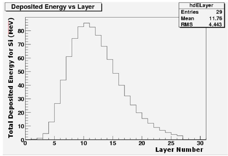
Figure 2.54: FCAL deposited energy as a function of the layer

In order to check the performance of FCAL, we used GEANT4 program to simulate FCAL. Figure 2.54 shows the energy deposited as a function of the layer for 100 GeV electrons hitting the detector. The shower maximum occurs at the layer 11 and small fraction of the energy is lost. Figure 2.55 shows the variations of the total energy deposited in the FCAL. Approximately the energy resolution($\Delta E/E$) of $23\%/\sqrt{E}$ is achieved for the 100 GeV electrons.

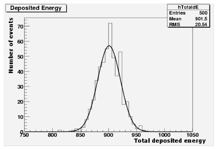
Figure 2.55: FCAL total deposited energy

The BCAL is located further downstream from the IP. It covers from $z$ = 430 cm to $z$ = 450 cm. It has a sampling structure similar to FCAL, except the fact that the air gap is 0.7 mm.

2.6.3 Pair Monitor

The current technology for PM adapts the 3-dimentional active pixel sensor, forming a double layer of silicon disks. It is located in front of the BCAL. The $z$ position of the PMis 400 cm and 401 cm from the IP. The inner radius of the disk is 2 cm and the outer radius reaches to 8.5 cm. It consists of an array of trapezoidal wedges, each composed by a sensor and a readout chip. There will be a large mount of $X$-ray hits from nearby devices such as quadrupoles, luminosity monitors that need to be removed either by requiring a coincidence between two adjacent wheels or by being able to set a clean 70 keV threshold per hit [41], thus reducing by 50 % the overall number of needed channels. Most of the created pairs will hit the central part of the monitor while $X$-rays are almost uniformlydistributed generating a background that needs to be removed in the external region where the monitor should withstand an occupancy up to 30% of created pairs per train crossing.

Beam instabilities are often caused by preceding bunches in a train: it is thus desirable to measure the beam profile for individualbunch or at least as a function of time from the beginning of train. It is also highly desirable that such information be available real time for machine tuning. The high occupancy suggests that silicon strip detectors are not suited for this application. A CCD sensor would be a good candidate in terms of occupancy; since the integrated charge deposit in each pixel is read out at the end of each train, however, the information on the location in a train is lost unless some external gating is applied. On the other hand, active pixel sensors can handle high occupancies just as CCDs and timing of hit can be digitized on each pixel. The 3D pixel design is particularly suited for this application for the following reasons:

• it is fast: the charge collection time is about 10 times faster than typical pixel devices, for a 50 $\mu$m pitch 3D cell where the ionizing track is midway between the central $p$ and corner $n$ electrode, perpendicular to the surface of the silicon crystal.

• it is radiation hard: the depletion voltage is of the order of 5 $V$ and has a large margin for increase by radiation.

• it has a flexible geometry and it can be easily made in a trapezoidal shape and the sensor can be active very close to the edge.

Each pixel sensor is bump-bonded to a readout chip which collects the charge, discriminates and time-digitizes it. The proposed pixel size is 100$\times$100 $\mu$m, thus its readout electronics has to fit in such a footprint.

2.7 Detector Magnet and Structure

2.7.1 Detector Magnet

Introduction

A superconducting solenoid magnet has been studied for the GLD detector. The required central magnetic field is 3 T in a cylindrical volume of 8 m in diameter and 9.5 m in total length. The stored energy is calculated to be 1.6 GJ. A 0.5 m length of correction coils is attached at both end of the solenoid coil to satisfy requirement of field uniformity. Because the magnet is planed to locate outside of the calorimeter, it is not necessary to design as a thin superconducting solenoid magnet. Therefore, the weight of the calorimeter estimated 2000 tons is planed to support at the inner wall of cryostat.

General Design

The magnet provides a central magnetic field of 3 T at nominal current of 7956 A in a cylindrical volume of 8 m in diameter and 9.5 m in length. The current density is about 60 percent of the critical current density. It is placed outside the calorimeter to achieve good hermeticity. The coil consists of double layers of aluminum stabilized superconductor wound around the inner surface of an aluminum support cylinder made of JIS-A5083(Figure 2.56). According to the detector requirements, the integrated field uniformity has to be less than 2mm. Thus 0.5 m length of four-layer coil is adopted at both of the coil. Indirect cooling will be provided by liquid helium circulating through a single tube welded on the outer surface of the support cylinder. Main parameters of the GLD solenoid magnet are summarized in Table 2.10. Radiation shields consist of 20 K shield and 80 K shield are placed between the coil and the vacuum vessel. These shields have to be decoupled electrically from both the coil and the vessel walls in order to avoid the effect of eddy current induced by the inner and the outer coaxial cylinders that are connected by flat annular bulkheads at each end.

Table 2.10: Basic parameters of the solenoid magnet.

Cryostat Inner Radius	3.72 m
Cryostat Outer Radius	4.4 m
Cryostat Half length	4.75 m
Cryostat weight	191 tons
Coil mean radius	4 m
Coil Half length	4.43 m
Cold mass	78 tons
Central magnetic field	3 T
Number of turns(2 layers)	2880
Current density	741 A/mm2
Nominal current	7956 A
Stored energy	1.6 GJ

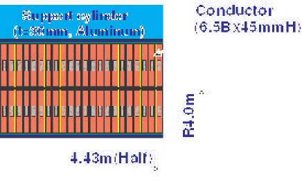
Figure 2.56: Cross section of the GLD solenoid magnet.

Coil Design

Superconducting wire for the GLD solenoid is based on the ATLAS superconducting wire. The size is scaled-up to 6.5mm width and 45mm height in order to absorb a magnetic force in the coil. The mechanical structure of the superconduction coil must sustain two main mechanical stresses, hoop stress and axial stress in the coil. The calculation results are shown in Figure 2.57 and the deformation of the coil when the solenoid excitation is shown in Figure 2.58. Even though the yield strength of superconducting wire is achieved to around 250 MPa at recent high strength superconducting wire development, it is assumed to yield strength of 150 MPa in this design. The combined stress, Von Mises, in the coil when the central magnetic field of 3 T is calculated to be 130 MPa. According to the calculation result, required thickness to keep within yield strength in the coil is to be 30 mm for support cylinder and 2 layers of 45 mm-thick for coil, respectively. From these required thickness, the cold mass is approximately 78 tons. The stored energy is calculated to be 1.6 GJ. The solenoid magnet will be supported at the innermost layers of barrel iron yoke by fixing the support structure on the outer vacuum vessel. The coil support system has to transmit both the weight of cold mass and the magnetic de-centering forces. If the geometrical center of the solenoid and the iron yoke are deviated, an unbalanced magnetic force is generated. So this force has to be taken into account on the coil support design. And another important requirement is that the coil supports have to follow the thermal shrinkage in the cooling down. The configuration of the coil supports is planed to adopt a rod type made of GFRP. In the de-centering calculation, a 380 tons in the axial direction and 130 tons in radial directions of de-centering forces act on the coil supports if the magnet and iron yoke is deviated 25 mm.

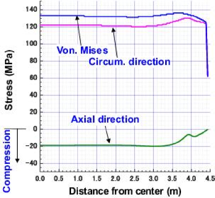
Figure 2.57: Stress distribution in the coil.

Figure 2.58: Deformation of the coil due to magnetic force.

Cryostat Design

Since the magnet is located outside of the calorimeter, it is not necessary to design as a thin superconducting solenoid magnet. Therefore, the weight of the calorimeter which is estimated to be 2000 tons is planed to support at the inner wall of cryostat. Load conditions for cryostat design are 2000 tons of self-weight of the calorimeter, 78 tons of cold mass, 380 tons of de-centering force on the bulk head and 0.1MPa of vacuum pressure. The cryostat material is assumed to be stainless steel. Thickness of the outer vacuum vessel can be calculated from the design guide line named NASA-SP8007. Then thickness of outer vacuum wall was calculated to be 60 mm with a safety margin of two. Figure 2.59 shows the calculation result when the weight of the calorimeter is suspended at horizontal positions of the inner wall. In this calculation, 60 mm of outer vacuum vessel, 100 mm of end plate and 60 mm of inner vessel were defined. The maximum stress is calculated to be about 118 MPa, this is below the allowable stress of stainless steel. The deformation is about 9 mm. In the seismic force calculation, load condition is 0.3 G of the self-weight of calorimeter is input to the horizontal direction of the inner vacuum wall. This result is 125 MPa of maximum stress and 9mm of deformation. One important thing in these calculations is that the calorimeter has a stiff structure. Otherwise, the self-weight of the calorimeter is placed on the bottom of the inner wall of the cryostat, which will cause the high stress level in the cryostat.

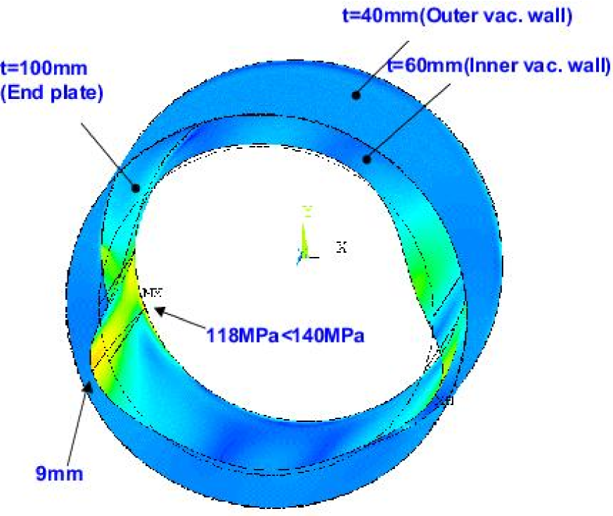
Figure 2.59: Stress distribution on the cryostat when a 2000 tons of self-weight of the calorimeter is supported at horizontal positions.

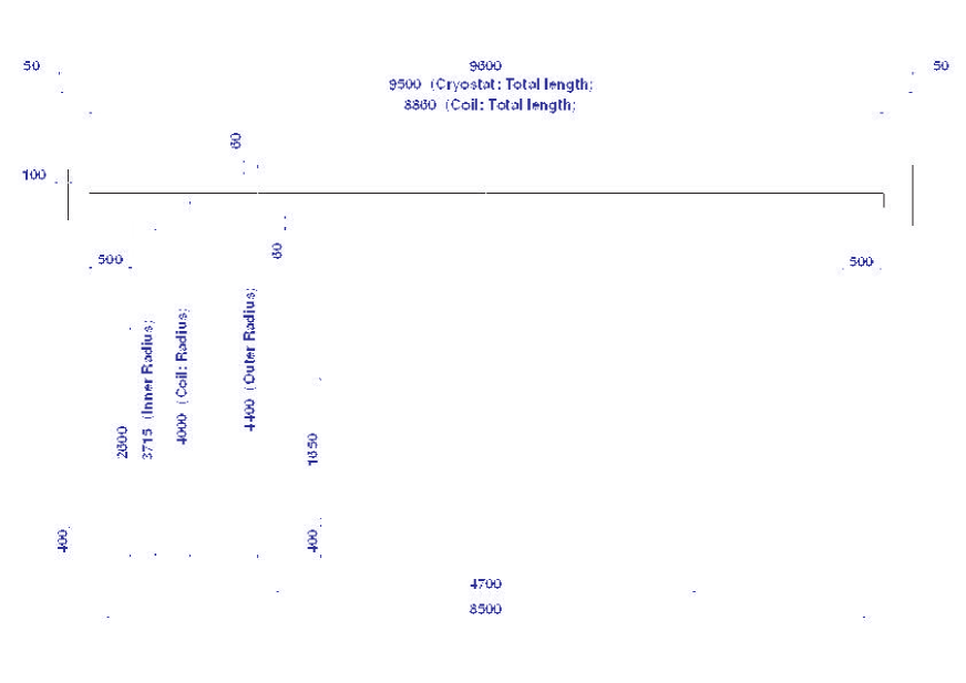
Figure 2.60: Half view of the GLD solenoid magnet.

Assembly Procedure

Drawing of the solenoid magnet is shown in Figure 2.60. Assembly procedure of the solenoid magnet will be similar to the ATLAS solenoid magnet. In that procedure, the superconductor is wound to the temporal mandrel with a cover by insulator at first. Then the coil winding is carried out after the temporal mandrel is set to the winding machine located inside the support cylinder. After this process, pure-al strips are mounted on the inner surface of the coil. The solenoid coil is completed after curing. Outer radiation shield is installed to the inside of the outer vacuum vessel. Then the coil with axial supports is installed. The inner radiation shield and inner vacuum vessel will be assembled. Then bulk heads are fixed. After the coil position is adjusted and the solenoid is laid down, the chimney is mounted. This work might be done after installation of the solenoid to the return yoke.

Conclusion

The GLD superconducting solenoid magnet has been studied. The coil design and superconducting wire design has mainly reported in this section. The thermal design and cryogenic design should be more investigated. In the mechanical design, support configuration of the solenoid magnet and the installation procedure should be carried out as the next step.

2.7.2 Structure

Introduction

An iron structure for the GLD detector has been studied and designed. The structure consists of the barrel and two end-yoke sections with dodecagonal shape. The overall height is about 17 m from the floor level; the depth is about 16 m. The iron structure will be made from low-carbon steel (JIS-S10C). The total weight except for sub-detectors is approximately 16000 tons, and it will be placed on the transportation system for roll-in/out. Assembling of the iron yoke and installation of the sub-detector will be carried out at the roll-out position and then moved to the roll-in position for the experiment. The end-yoke separates at its center and then opens to access the sub-detectors. Some kind of design studies are required to optimize the iron yoke configuration. Those are the influence of the magnetic field, stability against the acted force such as self-weight of iron yoke and assembling/maintenance consideration. In the magnetic field study, the iron yoke is acted on the magnetic field of 3 T from the GLD solenoid magnet, amount of iron have to be determined for improving the field uniformity in the TPC volume, and leakage field outside of the iron yoke is kept minimize by absorbing the flux return. In the mechanical design, it is required to study on the deformation and stress level against heavy self-weight of iron and strong magnetic force. As the other important issue for the mechanical design, an earthquake resistant design is required.

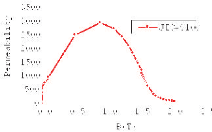
Figure 2.61: Input permeability for the magnetic field calculation.

Magnetic Field Design

There are two criteria for the magnetic design. One is integrated field uniformity in the TPC volume is less than 2mm. And another is leakage field at 10 m away from the solenoid center should be less than 50 gauss from the requirement of accelerator design. Between the barrel-yoke and the end-yoke, a 50 mm of air-gap is provided for passing though the cables from the inner detectors. With keeping these requirements, thickness of iron plates were tried to minimize as much as possible. Permeability of iron plate used for the calculation is the measurement data of the BELLE iron yoke as shown in Figure 2.61. The ways to improve the field uniformity without increasing the amount of iron are are to change the parameters of correction coil, which is located at the both ends, such as current density and coil length. Other ways are to change the radius and thickness of iron inside the solenoid. The distribution of magnetic field density is show in right-hand side of Figure 2.62. The calculated field uniformity is from -0.5 mm to +0.05 mm as shown in left-hand side of Figure 2.62. The magnetic field along the beam line is shown in Figure 2.63. The leakage field at 10 m away from the solenoid center is calculated to be 44 gauss. In this calculation, the outer two layers of return yoke has to be 50 cm-thick of iron plate to reduce the leakage field. From this calculation, each iron plate thickness of barrel and end-yoke can be optimized.

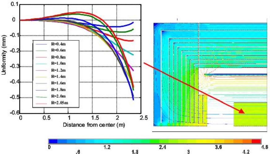
Figure 2.62: Field uniformity in the TPC volume.

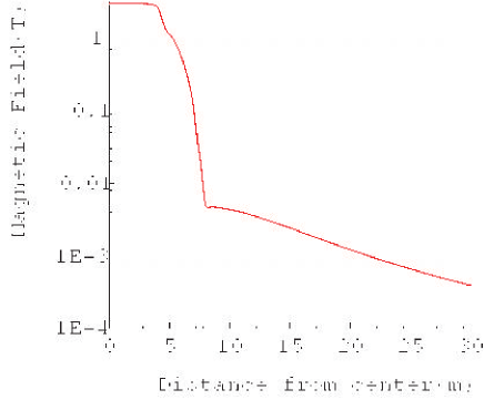
Figure 2.63: Leakage field along the beam axis.

Mechanical Design

The mechanical strength of JIS-S10C are 310 MPa of tensile strength and 205 MPa of yield strength, respectively. The iron yoke has to withstand against three kinds of load conditions. Those are self-weight, magnetic force and seismic force. The self-weight of iron yoke is estimated to 16000 tons. The barrel yoke is about 7500 tons and end-yoke is 8500 tons, respectively. The magnetic force is calculated to be 18000 tons. An input acceleration for the seismic design is applied 0.3G. The gravitational sag of barrel yoke is calculated to be 1.8 mm maximum. The stress level in the calculation was small enough. It is important to assemble with keeping the rigid structure. The gravitational sag of end-yoke is neglected. The deformation of the end-yoke due to the magnetic force of 18000 tons is shown in left-hand side of Figure 2.64. The maximum deformation was calculated to be 75 mm. Becausue this deformation can not be accepted, a support plate is required to reduce deformation and stress. The calculation result with 75 mm-thick of support plates are shown in the right-hand side of Figure 2.64. The support plate is mounted on every 90 degree. The deformation can be reduced to 1.8 mm. The result of seismic force is 2.8 mm in the horizontal direction.

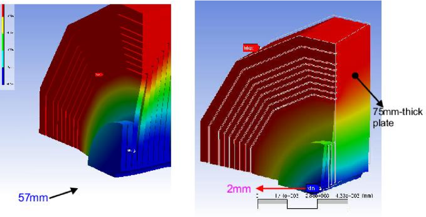
Figure 2.64: Stress contour display against magneic force.

Configurations

Drawing of the iron yoke is shown in Figure 2.65. The prefered shape of the yoke is a dodecagon from the viewpoint of the calorimeter design. There is a 50 mm air-gap between the barrel-yoke and the end-yoke as cable holes. So the barrel-yoke structure is constructed from twelve Muon modules. Each barrel Muon module consists of 9 layers with 50 mm thick instrumental gaps. Thicknesses of steel plates are 50 cm in outer two layers and 25cm in other layers, respectively. Few millimeters of flatness of steel plate should be taken into account on the Muon detector design. Each end-yoke is planned to separate into four quadrants containing eleven iron plates. Plate thickness of each layer is same as the corresponding plate of the barrel yoke. The end-yoke can slide out in order to provide an access to the inner detector. The iron yoke is sitting on an end-yoke transportation system.

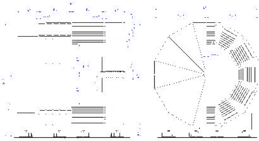
Figure 2.65: Drawing of the GLD iron yoke.

Assembling

Assembling procedure for the barrel-yoke is shown in Figure 2.66. Each Iron plates are bolted on the support frame. There are support jigs at each corner. Assembling will be done from the bottom side and the outer layer. At end-yoke assembling, each pieces divided to eight are assembled by welding. Because the end-yoke must withstand the huge magnetic force, each piece should be fixed rigidly. After completing each segment, end-yoke is assembled by bolting joints as shown in Figure 2.67.

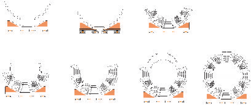
Figure 2.66: Assembling procedure of the barrel-yoke.

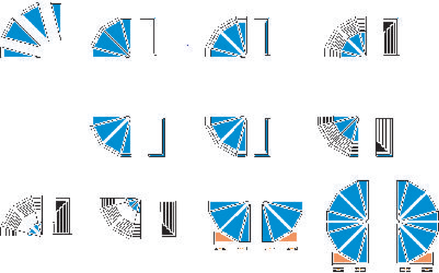
Figure 2.67: Assembling procedure of the end-yoke.

Experimental Hall

One of the request from the facility study team is that the smaller experimental hall is preferred from the viewpoint of the cost. To meat this request, a mechanism to open the end yoke is important. The way to open the end yokes at the experimental hall is to rotate the end-yoke by 90 degree like a door at first, then slide it along the beam direction about 10 m. Then, an access to the inner detector is possible. There are several kinds of moving devices available in the market, such as linear-guide system, air-pad system and so on. It is preferred to use an spherical roller table. Because the movement of the end-yoke is not only in one direction, i.e., including rotation and sliding. The spherical roller table can be used to move multi directions and air supply system is unnecessary. Figure 2.68 shows the experimental hall. The size of the hall is 72 m length, 32 m width and 40 m high. Two area, experimental area and maintenance area, are planed. The distance from the beam line and the nearest wall is 9 m.

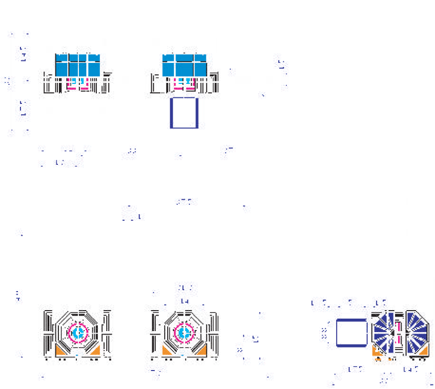
Figure 2.68: Floor plan of the experimantal hall.

Conclusion

In this magnetic field design, field uniformity and leakage field can be satisfied. Those are 0.2 mm and 40 gauss, respectively, and they are well below the criteria. To support the magnetic force on the end-yoke, 75 mm-thick of support plate is necessary even though effects of self-weight and seismic force are small. Parameters of the GLD iron yoke is summarized in Table 2.11. Based on the basic plan of the assembling procedure and the experimental hall presented here, more detail design is necessary.

Table 2.11: Parameters of the Iron Yoke.

Shape	Dedecagon
Air gap for Muon	5 cm
Uniformity(mm)	(-0.55) - (+0.05)
Leakage field	43 gauss(at 10m)
Barrel yoke	9 layers
End yoke	11 layers
Width	15.3 m
Length	16 m
Height	17 m
Barrel yoke	8250 tons
End yoke	4172x2 tons
Total	16594 tons

2.8 Data Acquisition

2.8.1 Introduction

In a first look, the data acquisition (DAQ) system for a ILC detector might be just a significant extrapolation, using more modern technologies than those used in all prior large scale, high energy physics collider experiments.

It should, a priori, be less demanding than the hadron colliders (Tevatron and LHC). ILC detector doesn’t have to cope with multiple minimum bias events per bunch crossing (BX) and high rate triggering for needles in a haystack, and radiation hardness is less critical. Hence many more detector technologies are available and better performance is possible. But, contrary to discovery machines, ILC detector does have to record all the observable information; measure jets and charged tracks with unparalleled precision, measure beam energy and its spread, differential luminosity and polarization, and tag all vertices, thus better performance and full hermiticity are needed in order to do physics with all final states.

Compared to previous lepton colliders (LEP, SLC and B-Factories) where jets and leptons are the fundamental quanta, they must be identified and measured well enough to discriminate between $Z$’s, $W$’s, $H$’s and possible new states. Challenging ILC physics goals requires to improve the jet resolution by a factor of two, and the excellent tracking capability for recoil mass measurements in the Higgs boson search, which requires 10 times better momentum resolution than LEP/SLD detectors and 1/3 better on the impact parameter resolution than SLD. To catch multi-jet final states (e.g. $t\bar{t}H$ can decay into 8 jets), the need of a real 4$\pi$ solid angle coverage with full detector capability is fundamental. Furthermore, the paradigm of “Particle Flow Algorithm (PFA)” for precision measurement of the jet energy requires an unprecedented fine-granularity calorimeter for good separation of charged and neutral particles. Such hermiticity and granularity have never been done up to now. Finally, the PFA also puts new challenge for real time analysis.

In summary, at the ILC the stringent requirements imposed by the high precision physics goals need a detector concept structure with full hermiticity, high granularity detectors with a DAQ able to select, analyze and store standard as well as rare events in a huge background environment. In addition, the high luminosity operation at the interaction point of the linear accelerator with two long independent arms needs to be optimized in real time using simultaneous information of both machine and experiment. These features put new requirements and challenges in this domain to be addressed.

From the conceptual point of view, the burst mode of the beam structure of the ILC machine (3000 BXs for a duration of roughly 1 ms at 5 Hz frequency) yields a BX rate of 3 MHz for 1 ms followed by a period of almost 200 ms without any interaction. That dictates immediately an innovative DAQ architecture with no hardware trigger.

From the technical point of view, the rapid development of computing and telecom technologies as well as the higher integration and lower power consumption of electronic components fits nicely with the requirements needed for all modern DAQ components. For such large and long-term life system, the uniformity of the various interfaces associated with standardized components is vital to achieve flexibility, maintainability, scalability at an affordable effort, requiring commodity hardware and industry standards to be used wherever possible.

Therefore, and partly because of the rather much dependence of the detector design, the DAQ system presented at this stage is only a conceptual model with some basic principles to be refined later, for example, the implementation of special non machine synchronized triggers such as Calibration, Cosmic. However, its aims is to define clearly the common and uniform interfaces between the various logical components and to show the feasibility of the system in general.

2.8.2 Event Selection System (Trigger)

The main goal of event selection system (Trigger) is to select interesting events in the presence of several orders of magnitude higher background without losing data of a possible, yet unknown, physics process. In addition the rates of the known interesting physics processes vary as well by several orders of magnitude. The ILC operation conditions are quite different from those of accelerators currently operating or being constructed. The main ILC parameters of the 500 GeV present design, relevant for the DAQ system, are:

• a long time interval between two bunch trains of 200 ms,

• a separation of two bunches inside a train by 308 ns,

• a train length of 868 $\mu$s.

These conditions drive the proposal of an event building without any hardware trigger, followed by a fully software based event selection, identification and analysis. This concept allows to analyze each event one by one without taking into account a fixed trigger latency as it is done in the standard experiments.

To achieve a dead-time free data acquisition under the ILC operation conditions, a trigger-free pipeline of 1 ms with readout of all data in the pipeline within 200 ms is proposed. The full data paths and data flow is presented in the Figure 2.69.

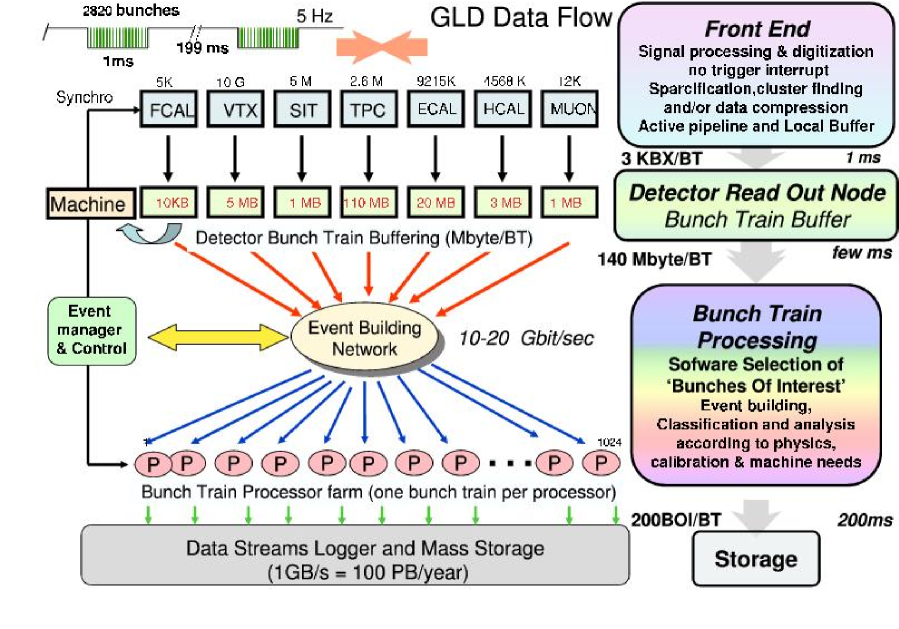
Figure 2.69: Schematic view of the data paths and data flow in the DAQ system.

In the first step, during the 1 ms bunch train of 3000 collisions, each detector channel signal is digitally processed at its front end without any trigger interrupt. During or immediately after this, 1 ms active pipeline, depending on the detector type, the raw data throughput will be reduced directly at the subdetector front end level by implementing the usual data compression tools and algorithms like zero suppression, sparcification, hit detection or cluster finding before storing the relevant data fragment in a local buffer.

In a second step, during the first part of 200 ms available with no beam, a collection of all the data in the full bunch train is performed. Each locally stored front end data fragment is digitally multiplexed in a reasonable quantity of fast read out links and then pushed to a series of Bunch Train read out Buffer (BTB) mapping each detector. After the necessary time of data collection estimated few ms, which is compatible with the power cycling of the font-end electronics, the complete collection of the full bunch train data is performed by one processing element, the Bunch Train Processor (BTP) of the online farm, prior to a software selection of Bunches Of Interest (BOI) using a specific set of raw data followed by an event classification according to physics, calibration and machine needs. The only constraint in this model is that the data collection task should be made within the $\sim$190 ms, remaining several ms before the next bunch train, in order to free all the read out buffers (BTB’s), however the rest of the treatment could be longer since the following bunch train will be analyzed in another processor. This scheme of merging all the processing tasks from the event builder and event finder in one processor unit, avoids to move data several times and makes event management and control easier.

The evolution of embedded processing power and network will allow to merge in this processor all the successive software tasks, accomplished today in large experiments like the so-called Level 2 (L2), Level 3 (L3), High Level Trigger and Filter (HLT), up to the first full reconstruction and physics analysis using the PFA of each BOI event. In addition the standard real time monitoring tasks should be performed like calibration and alignment for the detectors as well as complete analysis of sampled events. From the total hadronic cross section for $e^{+}e^{-}$-annihilation, about 0.1 for high $Q^{2}$ events per train are expected and 4 for Bhabha whereas about 200 events per train will come from $\gamma\gamma$ reactions. All these events are potentially interesting, e.g. $\gamma\gamma$ and low $\Delta M$ SUSY are very difficult to distinguish, and a systematic storage of those candidates might be necessary prior to a complex analysis carried out later on. Assuming a rate of 200 BOI selected per bunch train and processing time of 1 second per event in average to perform all these analysis tasks, a farm of 1024 processors would be necessary.

2.8.3 DAQ Boundaries and Read Out Architecture

One of the most important tasks in the development of a DAQ system for the GLD detector is the choice of a coherent architecture that meets the requirements of all subdetectors. The system cost will be minimized and the reliability and ease of debugging optimized if an architecture is chosen that is uniformly applied. The requirements for the GLD DAQ system fall into four broad categories. First are the quantitative requirements such as those on the bandwidths of data paths and the number of data sources and data volume to be accommodated. Second are the important architectural requirements that allow front end systems and event selection to be operated together or independently. Third are the requirements for initializing, controlling and monitoring the system. Last are the qualitative requirements for items such as reliability, tolerable error rates and maintainability. All these requirements can be grouped in four functional blocks and their interfaces.

Detector Front End Electronics (DFE)

The term of front end electronics is broadly used to denote the electronics that is physically located within the GLD detector. Its basic purpose is to convert sets of signals from each detector element into digital event fragment. The signal processing typically contains low-noise, high time resolution amplifiers and signal shapers. Each amplifier receives a signal, almost always an analog signal, from one sensor element such as pixel, Si strip, TPC, SiPM/MPPC. The signal is shaped in order to extract the best quality time and/or amplitude information from the input signal. Digitization or quantization occurs immediately after this stage. The provision for generating calibration signals is typically made. This feature can be used for channel time and/or amplitude calibration by inserting artificial sets of data to test all or part of the electronics chain. The signal must be preserved within the front end system for the 1 ms bunch train. The front end electronics system of the GLD detector will be implemented in various ways, depending on the sensor type.

The impact of a 1 ms active pipeline without trigger interrupt and therefore no possibility of a fast clear or buffer flushing for the different subdetector pipelines has been studied and readout technologies able to cope with this have been proposed for several detector technologies. For the vertex detector built in CCD technology, a column parallel readout at a speed of 50 MHz during the active pipeline has been proposed to handle the expected data rates. For the TPC several designs are being studied which allow the collection of signals in an ungated mode for the full time of the pipeline by limiting the ion feedback with Micro Pattern Detector read out (GEM, Micromegas), and for the scintillator devices (EM and hadron calorimeters and muon detector), built out of silicon avalanche photodiode, a continuously running pipeline with hit detection and multiplexing is foreseen. The uniform interface between the DFE and DAQ system is the Local Detector Buffer (LDB).

Machine Detector Interface (MDI)

The adjustment of the luminosity should be carried out at the beginning of each bunch train. The current thinking is to use the very forward calorimeter (BCAL) raw data of about 10 to 50 bunches to get an immediate feedback for the machine. Accordingly, the forward calorimeters have to be read out at each bunch crossing and the readout philosophy is different from the rest of the detector elements. Other complex information can be sent during the full bunch train analysis of specific background events. Another feature connected to the machine are the bunch synchronization and distribution.

Data Acquisition (DAQ)

This is the central part of the system. It is divided functionally into three main architectural components, the read out node, the network switch and the bunch train processor (BTP) farm.

The read out node associated with one detector collects all the data fragments in one bunch train into a Bunch Train Buffer (BTB). This is done by regrouping and multiplexing the various front end local buffer scattered inside and around the GLD physical structure in a minimum number of fast data links. Building the bunch train sub events as well as checking the integrity of its content requires some intelligence and fast connectivity at that level that controls all relevant tasks associated with one detector. This is a networking hub where a uniform interface across all the various detectors between the front end electronics and the DAQ should be installed. Today, it will be done using PCI mezzanines with powerful FPGA’s embedded on VME or PC boards.

The network switch with a typical capacity of 10-20 Gbit/sec will be adequate to collect and distribute the full bunch train data, estimated today at 140 MBytes, to the designated Bunch Train Processor.

The event building will be performed at 1-2 GByte/sec and the Bunch Of Interest selection can select up to 250 events including the $\gamma\gamma$ physics processes as well as additional calibration and background events for cross checks. The event size varies from 0.2 MBytes to 5 MBytes, depending on the amount of background included. Assuming background data to be suppressed, the processed event size will be on average about 1 MByte which leads to 250 MByte/sec output to be transfer to the mass storage. This results in a total data volume of roughly 1 GByte/sec or 10 PByte/year, e.g. 10 times the LHC production. This seems a little bit too much and more study is needed to reduce this data volume in an unbiased way. Considering that 90% of the data are produced by TPC, calorimeters and VTX and that most data volume is background, some reduction would be possible to clean up event by removing noise hits, using the time stamp on one bunch crossing and recording only interesting regions or tracks. A rough qualitative analysis of this issue would expect a reduction of a factor of 5 to 10.

Compared to systems built for the LHC experiments, the proposed DAQ system for GLD is less demanding and key components like the fast switching network and the computing units are available already today.

Global Detector Network (GDN)

The international worldwide structure of the ILC/GLD collaboration combined with the fantastic development of fast communication tools allows us today to imagine a new way in High Energy Physics to gain control of the experiment from the detector calibration and monitoring to the physics analysis.

With the exceptions of the detector integration and commissioning, the rest of the detector operation, in particular data taking and its associated services (ancillary controls, partitioning, databases management, …), can be distributed among several virtual control rooms. It would be possible to select from these remote stations the running modes between stand alone, cosmic test, calibration and global runs without coming to the detector site in person, as is done for many embedded satellite experiments.

From the physics analysis point of view, the boundaries between so-called online and offline will disappear and the development of GRID technologies shows that it will be possible in the future to analyze data without knowing where the processing is made.

Technologies Forecast

The fast development in the computing and network area makes it difficult to predict the technologies which will finally be used to build the DAQ system in several years from now. A short overview of possible evolution of technologies is presented below, based on past experiences, current running experiments and studies for the experiments planned at the LHC.

Concerning the Standards: this is the end of traditional parallel backplane bus paradigm (CAMAC, Fastbus, VME). It has been announced every year since $\sim$1989, but still there at LHC with VME and PCI. Recently, a new commercial standard has been emerging from the telecom industry named Advanced Telecom Computing Architecture (ATCA) designed for a very high system throughput (2 Tbit/sec) and availability (99.999%, failure rate of $\sim$5 min/year). It has the technical features well suited for all our needs particularly to host the detector bunch train read out hub as well as the basic components of the machine control. The basic software is already available under Linux.

The commercial networking products for Trigger/DAQ switches was already available in the 90’s: ATM, DS-Link, Fibre Channel, SCI, etc. Today, the Gigabit Ethernet is the most popular with the rapid bandwidth evolution from 1 Gbit/sec to 10 Gbit/sec and with the objective to reach 30 Gbit/sec in 2010.

The ideal fast processing / memory / IO bandwidth devices existed in the past: Transputers, DSP’s, and RISC processors. Today, there are powerful FPGA’s that integrate everything: the LVDS receiver links, DSP’s, large memory, as well as more general purpose processors like PowerPC.

For the point-to-point link technology, the old style used even recently at LHC was parallel copper or serial optical. The recent evolution is to go toward the serial copper and parallel optics. The link speed is $>$ 3 Gbit/sec today and 10 Gbit/sec is in demonstration.

The continuous increasing of the computing power for the processor power and clock (today 4GHz, 10 to 15 GHz foreseen in 2010) is not anymore a critical issue. Idem for the memory size which is now quasi unlimited (blocks of 256 MB today, few GB in 2010).

In conclusion, the evolution of technologies described above shows that there will be adequate components when the final decision has to be made.

2.8.4 Strategy for the Future

Previous experiences of DAQ systems demonstrate that the final technologies and their associated commercial components should be chosen as late as possible, e.g. 3–4 years before the first beam collision. However, the architectural model with its functional blocks and interfaces should be adopted as early as possible in order that the various detectors could develop the necessarily uniform interfaces at the front end electronic level. Hence, the basic idea is to organize the DAQ development around a common pilot project across the various concepts and detector R&D. This pilot project should address all the main issues and also details attached to the conceptual model described above, such as the integration and feedback of the machine and its synchronization, slow controls, non machine synchronized acquisition modes like calibration, test and cosmic trigger. It is also the place where state of the art technologies like ATCA could be practiced and evaluated. Finally, the worldwide aspect of such pilot project will be a learning process for developing and optimizing all the Global Detector Network functionalities.

2.9 Machine Detector Interface

2.9.1 Background Tolerances in GLD

Background tolerances of the vertex detector (VTX), the TPC, and the calorimeter (CAL) are estimated in terms of tracking capabilities and radiation hardness. The tolerances depends on readout time or sensitive time of detectors, which are O(1) msec, 50 $\mu$sec and 100 nsec for FPCCD VTX, TPC and CAL, respectively.

To achiveve a good efficiency in track reconstruction, the occupancy in the vertex detector are required to be less than 1%. Major background sources are $e^{\pm}$ pairs and neutrons backscattered at the extraction beam line.

The tolerable hit densities of pairs and neutrons of the vertex detector are $1\times 10^{4}$/cm²hits/train and $1\times 10^{10}$n/cm²/year, respectively, where a train have 2820 bunches with time separation of 307.7 nsec. The hit rate corresponds to 1% occupancy.

The TPC has $2.46\times 10^{9}$ voxels in total, consisting of pads and time-buckets. Tolerance of background hits is estimated to be 0.5% occupancy, that is $12.3\times 10^{6}$ voxels/50$\mu$sec, where the 50 $\mu$sec is a full drift time in the TPC. Assuming a hit has 5(pads)$\times$5(buckets), the tolerance cab be expressed by $5.02\times 10^{5}$ hits/50$\mu$sec. From this evaluation, tolerance of muons can be estimated to be $1.23\times 10^{3}$ muons/50 $\mu$sec assuming that a muon creates 2000 hits in the bucket of a single pad. Neutron tolerance can be estimated to be $4\times 10^{4}$ n/50 $\mu$sec assuming that a neutron creates 10 hits assuming 100% efficiency for neutrons to make hits which is so called neutron conversion efficiency. Since the efficiency depends on the gas content, it has been estimated to 1% with P10-gas in the TPC.

Muons can be serious background in the endcap calorimeters since they hit all the layers and mimic tracks. Signals can be read out with 100 nsec gate in the calorimeters. Only one muon can be allowed in the endcap calorimeter of 30 m² within the gate. Therefore, tolerance of muons is 0.03 $\mu$/m²/100 nsec .

The tolerances are listed in Table 2.12. They should be further investigated by the full simulation of Jupiter.

Table 2.12: Tolerances for background in VTX, TPC and CAL.

Detector	Hits	Neutrons	Muons
VTX	$1\times 10^{4}$ hits/cm2/train	$1\times 10^{10}$ n/cm2/year	-
TPC	$5.02\times 10^{5}$ hits/50$\mu$sec	$4\times 10^{4}$ n*/50 $\mu$sec	$1.23\times 10^{3}\mu$/50 $\mu$sec
CAL	1 hits/m2/100 nsec	-	0.03 $\mu$/m2/100 nsec

2.9.2 Interaction Region (IR) Design

IR geometries, especially the beam pipe and the innermost radius of VTX, depend on the machine parameters such as beam energy, intensity and sizes at the interaction point (IP) as well as crossing angle, distance from IP to the final quadrupole magnet (L*) and the detector solenoid field (B). While the accelerator can be seamlessly operated in the parameter space[6, 42], the present designs were optimized with all the parameter sets at E${}_{cm}=$500 GeV and 1 TeV, L* = 4.5 m and B = 3 Tesla for physics and background studies. As explained in the VTX section, the beam pipe inner radius has been determined from the IP to the final focus quadrupole magnet (QD0) by the envelope of pairs [43]. The configuration of beam pipe is shown in Figure 2.70. The detailed geometrical data are listed together with the extreme cases of the high luminosity parameter sets and the improved one at E${}_{cm}=$1 TeV [42] in Table 2.13 . The innermost VTX layer is located to be 0.4 or 0.5 cm from the beam pipe, e.g. its radius is 1.7 cm with the beam pipe of 1.3 cm radius at the nominal set. The standard radii of beam pipe and the innermost VTX layer are 1.5 cm and 2.0 cm, respectively, for the Jupiter simulation.

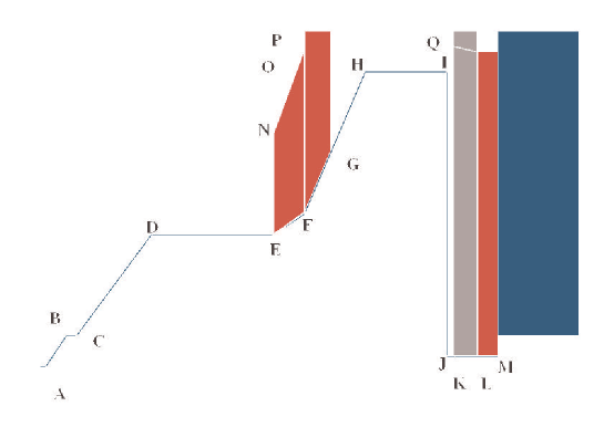
Figure 2.70: IR Geometry, where red-region is calorimeter (FCAL and BCAL), the grey one is a CH₂ (low Z) mask and the blue is the final quadrupole magnet(QD0). A pair monitor is set in front of the CH₂ mask, i.e. between J and K.

Table 2.13: IR geometrical data with 2 (20) mrad crossing angle; numbers in parentheses are those at 20 mrad crossing angle, while the others are common at the both angles.

Ecm	500 GeV				1 TeV
para.set	Nominal		High Luminosity		High Luminosity-1
position	R in cm	Z in cm	R in cm	Z in cm	R in cm	Z in cm
A	1.3	4.5	1.9	6.3	1.5	5
B	3(3.2)	25	4.2	25	3.4(3.5)	25
C	3(3.2)	35	4.2	35	3.4(3.5)	35
D	8	110	9(10)	110	8(9)	110
E	8	230	9(10)	230	8(9)	230
F	9.04	260	10.2(11.3)	260	9.04	260
G	11.94	285	12.60(13.26)	285	11.94(12.60)	285
H	16	320	16	320	16	320
I	16	400	16	400	16	400
J	2(2*)	400	2(2*)	400	2(2*)	400
K	2(2*)	405	2(2*)	405	2(2*)	405
L	2(2*)	430	2(2*)	430	2(2*)	430
M	2(2*)	450	2(2*)	450	2(2*)	450
N	13	230	14(15)	230	13(14)	230
O	17.70	260	18.83(19.96)	260	17.70(18.83)	260
P	36	260	36	260	36	260
Q	17.96	430	19.83(21.70)	430	17.96(19.83)	430

* : There are two holes with the same radius for incoming and exit beams at the 20 mrad crossing angle.

2.9.3 Collimation Aperture

Synchrotron Radiation

Since the beams are accompanied by halos, they should be sharply collimated at the collimation section at upstream in the beam delivery system. The halo particles generate synchrotron radiations in magnets and muons at the collimators. Collimation apertures have been optimized for the radiation profile to be small at IR region in order to prevent the direct hits at beam pipes and inner surfaces of the final focus magnets. We adopt the collimation scheme by A. Drozhdin [44]. The apertures are set to be $8\sigma_{x}\times 65\sigma_{y}$ . The properties of major collimators are listed in Table 2.14, where absorbers ( 30 X_o at least ) are installed behind the spoilers of SP2, SP4 and SPEX . Two masks of MSK1 and MSK2 are set to shield IR region against synchrotron radiations at downstream of the last bend magnets which are located at 96 m from IP.

Table 2.14: Major collimators’ location from IP, aperture, length and material (ILCFF9).

name	Location	Thickness	Material	Aperture
	m	Xo		x(mm)	y(mm)	x($\sigma_{x}$)	y($\sigma_{y}$)
SP2	1483.27	0.6	Copper	0.9	0.5	8	65
SP4	1286.02	0.6	Copper	0.9	0.5	8	65
SPEX	990.42	1	Titanium	0.5	0.8	10	62
MSK1	49.81	30	Tungsten	7.8	4.0	16	178
MSK2	13.02	30	Tungsten	7.4	4.5	12	151

The synchrotron radiations have been simulated by a Monte Carlo program of LCBDS [45] based on GEANT4. Transverse profiles of the radiations are shown in Figure 2.71, where beams have two components of core and halo. The beam halo were created by Gaussian distributions with standard deviations of $50\times\sigma_{x(x^{\prime})}$ and $200\times\sigma_{y(y^{\prime})}$, where $\sigma_{x(x^{\prime})}$ and $\sigma_{y(y^{\prime})}$ are those of the core distribution. No halo particles hit the beam pipe at IP, since they are collimated within radius of 1 cm.

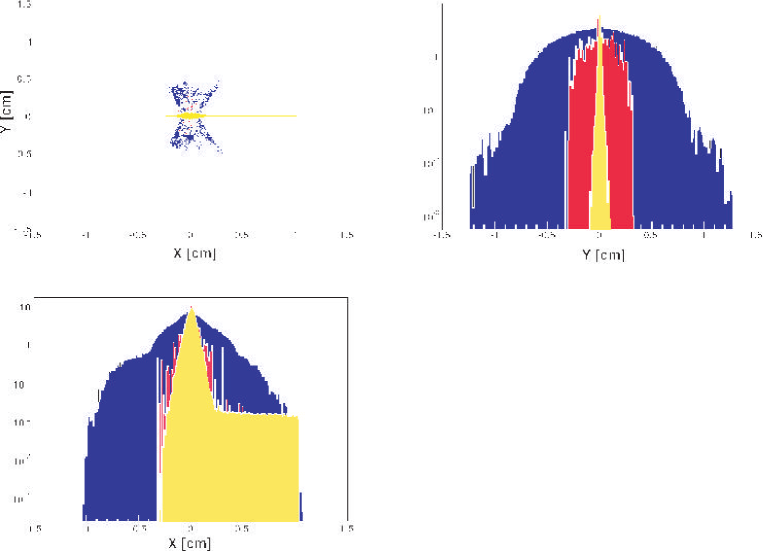
Figure 2.71: Synchrotron radiation profiles at IP, where yellow and red parts show the profiles of beam-core and -halo with the collimators, while blue part shows those without MSK1 and MSK2. Vertical scale in projected figures (right and bottom) is an arbitrary unit. The nominal parameter set has been used for this study at E_cm = 500 GeV, L* = 3.5 m and 20 mrad crossing angle.

Muons

Two muon spoilers are the baseline configuration to reduce muon flux by $1\times 10^{-4}$ in the ILC-BCD [46]. They are so-called ”tunnel fillers” of 9 and 15 m thick magnetized irons at 660 ad 350 m from IP, respectively. The rate has been estimated to be 0.8 muons/150 bunches in detectors with the beam halo of $10^{-3}$ [47].

The alternative approach of muon attenuators has been investigated in the ACFA-LC working group [2] . Since the beam delivery system in the previous study [48] is very similar to the ILC one, the major results can be borrowed in this report. All the empty beam line is covered by the attenuators which is consisted of two coaxial iron pipes of 8 cm and 78 cm diameters around the beam pipe of 2 cm diameter. The iron pipes of 244 m toal length are magnetized at 1 Tesla. As shown in Figure 2.72, the reduction factor of muon flux is close to that with the muon spoilers.

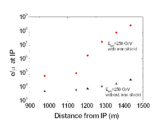
Figure 2.72: Number of electrons to produce one muon reaching the IP as a function of muon creation point, this figure is the same one in the GLC Project, p.235 [48].

We are investigating the muon background by using LCBDS.

2.9.4 Crossing Angle and Final Quadrupole Magnet

Two crossing angles have been set to be 2 and 20 mrad as the baseline configuration in the Baseline Configuration Document [46]. Also the baseline designs of final focus quadrupole magnet have been chosen to be a large bore super-conducting (SC) and a compact SC magnets at the 2 and 20 mrad angles, respectively, while permanent magnets are the alternative ones for the both angles. Their major geometries are listed in Table 2.15 which are used in the simulation studies.

Table 2.15: Various types of QD0 and the first quadrupole magnets at the extraction line, which are relevant in IR region: properties used in the simulation, where L* is the distance from IP and QX1A and QDEX1A at the extraction line.

type	Crossing angle	L*	Length	Aperture	Outer diameter
	mrad	m	m	cm	cm
Large SC	2	4.51	2.5	7	42
Permanent	2	4.51	2.5	2	18
Compact SC	20	3.51	2.2	2	6.1
Permanent	20	3.51	2.2	2	10
QX1A	20	3.51	2.2	2.6	4.78
Compact SC	14	4.51	2.2	2	7.2
QDEX1A	14	6	1.64	3.6	9.2

With small angle crossing, the most crucial issue is an energy deposit at the SC-QD0 in the extraction beam line. Sources of the energy deposit are pairs, disrupted beam and radiative Bhabha events. The pairs hit uniformly inside of the QD0 for their low energies, , while the disrupted beam hit more at the downstream for higher energies. Table 2.16 lists energy deposits due to the pairs at QD0 with 2 mrad crossing angle for the parameter sets, which were calculated by LCBDS. There should be no problem in the cryogenic power with these heat losses at any parameter sets.

Tolerance of the energy deposit in the SC magnets can be expressed in a unit weight, that is 0.5 mW/g to break the superconducting state. Since this tolerance has been estimated for the DC deposit, the ILC bunch-train structure may have more tolerable one. The simulation shows that pairs deposit energies of less than the tolerance for all the parameter sets even at E_cm = 1 TeV while the disrupted beam exceeds it in cases of the High Lum a E_cm = 500 GeV and the Low P, High Lum at E_cm=1 TeV. The High Lum-1 has the marginal deposit energy at High Lum at E_cm = 1 TeV. This issue requires further study to optimize the configuration of SC-QD0 with 2mrad crossing angle.

Table 2.16: Energy deposits in unit of mW, at QD0, 2 mrad crossing angle, where values in parentheses are those for two beams to collide with horizontal offset of 200 $\sigma_{x}$.

Ecm	Nominal	Low Q	Large Y	Low P	High Lum	High Lum-1
500 GeV	93(112)	80(76)	107(103)	158(146)	435(398)	-
1 TeV	464(513)	464(437)	769(687)	928(828)	2180(2260)	1170(1090)

With 20 mrad crossing angle, energy deposits were calculated to be 43mW due to the pairs at first extraction quadrupole magnet ( QDEX1 ) which is located at 3.5 m from IP. The QDEX1 has aperture of 2.6 cm, outer-diameter of 4.78 cm and length of 2.2 m as listed in Table 2.15. Since disrupted beam can be focused separately from incoming beam at the QDEX1, it will not deposit energy more than the tolerance with all the parameter sets.

The permanent magnet must be very robust against radiations and the energy deposit. The typical demagnification is 0.3% with $1\times 10^{13}$n/cm² [49]. In addition, it does not generate artificial vibration for no cooling water and neither electricity. Therefore, it must be a good alternative option for the QD0 [50] . Since the permanent QD0 is compact, the disrupted beam can be extracted outside of it as similar to the compact SC one at 20 mrad crossing angle, where the extraction line has the same configuration as the baseline. In case of 2 mrad crossing angle, the energy deposit is expected to be greater than the large SC because of smaller aperture for pairs and disrupted beam. However, the radiation damage must be irrelevant. Such performances will be investigated by the full simulation together with the hardware R&D.

In the case of 20 mrad crossing angle, the Detector Integrated Dipole (DID) has been proposed in order to tune the beam orbits with level collisions, i.e. zero vertical angles, at IP [51] as well as to reduce the synchrotron radiation effects on the beam sizes. After SNOWMASS 2005 the intermediate crossing angle of 14mrad has been investigated as the alternative one for less effects on the orbits and the radiations. Taking account of these improvements, anti-DID, which has opposite sign of the DID magnetic field, was proposed at the 14 mrad crossing angle. An optimization of interaction region was presented at the NANOBEAM 2005 [52].

In next section, we evaluate the DID and anti-DID in terms of backgrounds by simulations.

2.9.5 Background

Hits in VTX and TPC

The incoherent pairs and disrupted beams have been generated with the machine parameter sets by CAIN. Background hits from them have been calculated by the full detector simulation of Jupiter as well as the LCBDS . Present results are very preliminary for limited statistics of the simulation and without optimization of detailed geometries, where a single bunch collision has been simulated with the parameter sets, 2 mrad and 20 mrad crossing angles and anti-DID at E_cm = 500 GeV.

The VTX hit density in the first layer may exceed the tolerance ( $10^{4}$/cm²/ train ) at the high luminosity parameter sets, where the results have large statistical errors. There are more hits at the outer layers at 20mrad than those of the 2 mrad. The anti-DID actually reduced the hit densities at the outer layers close to the 2mrad cases .

Number of TPC hits may exceed the tolerance ($2.46\times 10^{5}$hits/50 $\mu$sec) with the high luminosity and the low P sets and the tolerance is marginal with the 20 mrad crossing cases. The anti-DID reduces the number of TPC hits below the tolerance, especially in case of the high luminosity. The low Q parameter set has less hits by more than twice than the nominal one in VTX and TPC.

Energy Deposit in BCAL, Beam Dumps and Neutrons

Neutrons are created by electromagnetic energy deposit in materials with typical rate of 130 neutrons(n)/TeV, which corresponds to $10^{9}$n/J . The pairs, disrupted beams and beamstrahlung photons hit the calorimeters (BCAL), magnets at the extraction line and the beam dumps, where they deposit energies for neutrons to be created. The neutrons are backscattered into the VTX around IP. Assuming they scatter uniformly in all solid angle, their flux density at the VTX (IP) is in inverse proportion to L², where L is distance from the creation point to IP. The tolerance is estimated to be $10^{10}$/cm²/year in the VTX. With the above consideration, tolerable energy deposit can be expressed by E = 0.13 L² with E in Watt(W) and L in m, e.g. 0.13 W and 1 KW at L = 1 m and 88 m, respectively.

Energy deposits in BCAL are listed with various conditions in Table 2.17 .

Table 2.17: Energy deposits due to the pairs in BCAL with the 2 mrad crossing angle, where the unit is Watt (W) and values in parenthesis are those at the 20 mrad crossing angle. The tolerance is also listed at BCAL, L = 4.3 m from IP, which is calculated by E = 0.13 L².

Ecm	Nominal	Low Q	High Lum	High Lum-1
500 GeV	0.05(0.10)	0.03(0.07)	0.27(0.42)	-
1000 GeV	0.12(0.22)	0.07(0.16)	0.68(0.94)	0.32
tolerance	2.4

In reality, a fraction of neutrons comes out in backward from the material. Therefore, the above estimation is the conservative limit of energy deposit from the VTX damage. For examples, it has been shown that neutrons were backscattered from the nearest quadrupole magnet in JLC detector with rates of 8.1 n/TeV and 36 n/TeV by simulations of GEANT3 and FLUKA, respectively [2]. In this case, the fractions are 0.06 and 0.28, respectively. Also the fraction from the water beam dump was estimated to be $1.67\times 10^{-4}$.

At ILC, total energy deposit is 23 MW at the beam dump. Since the dump is located at 650 m and 300 m from IP at the 2 mrad and 20 mrad crossing angles, respectively, the tolerances are estimated to be 330 MW and 70 MW, respectively, with the fraction of the water dump. Therefore, the beam dumps should not be relevant in the VTX radiation damage. Energy deposits will be investigated at the extraction line.

Chapter 3 Physics Performance

3.1 Tools for Studies of Physics Performances

The detector configuration used for physics performance studies of the GLD detector presented in this chapter is summarized in Table 3.1. A cut view of the detector is shown in Figure 3.1. The studies used the software modules QuickSim, JUPITER and SATELLITES implemented in the JSF [55] framework unless specified otherwise. These tools are described briefly in this section before describing results in the subsequent sections.

JUPITER [55] is a full detector simulator based on Geant4 [54]. For this study, we used version 7.0patch1. JUPITER provides a modular structure for easy update and installation of sub-detector components. To this end, powerful base classes have been developed including: a unified interface to facilitate easy installation of detector components, classes to help implementation of detailed hierarchical structures, automatic naming system and material management to minimize user-written source codes, and a mechanism to compose magnetic fields of many accelerator components. Detector configurations are defined by a external text file to allow easy modification of detector configuration.

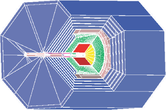
Figure 3.1: GLD Detector Cut View

Table 3.1: The standard geometry parameter used for JUPITER simulation.

Component	Specification
Beam Pipe	Inner Radius 1.5 cm, Be, 250 $\mu$mt
	Outside IP region($|Z|>5.5$ cm, Al. 2 mmt
VTX	6 layers of Si cylinders, 50 $\mu$mt each
	Inner Radius (cm) : 2.0, 2.2, 3.2, 3.4, 4.8, 5.0
	Half Z Length (cm) : 6.5, 6.5, 10.0, 10.0, 10.0, 10.0
	Resolution : $\sigma_{r\phi,z}$ = 4 $\mu$m
IT Barrel	4 layers of Si cylinders, 560 $\mu$mt
	Inner Radius (cm) : 9.0, 18.5, 28.0, 37.5
	Half Z Length (cm) : 18.58, 38.20, 57.81, 77.43
	Resolution : $\sigma_{r\phi,z}$ = 10 $\mu$ m
IT Endcap	7 layers of Si disks, 560 $\mu$mt
	Inner Radius (cm) : 2.5, 4.5, 7.0, 8.0, 10.0, 12.0, 14.0
	Outer Radius (cm) : 7.0, 14.0, 21.0, 28.0, 36.0, 38.0, 38.0
	Z position (cm) : 14.5, 29.0, 43.5, 58.0, 72.5, 87.0, 101.5
	Resolution : $\sigma_{r\phi,z}$ = 10 $\mu$m
TPC	Sensitive Region : $43.715cm<r<197.765cm$, $|z|<255cm$
	Gas: P10
	Inner TPC Support : 4.215 cmt, 0.013$X_{0}$
	Outer TPC Support : 8.235 cmt, 0.017$X_{0}$
	TPC End Plate : 5 cmt, $0.1X_{0}$
	Number of radial sampling : 200
	Resolution : $\sigma_{r\phi}$ = 150 $\mu$m, $\sigma_{z}$ = 400 mm
CAL	Tower structure,
	Inner radius of Barrel : 210 cm
	Front Z position of Endcap : 270 cm
	Coverage : $|\cos\theta|<0.98$
	Tower size EM 4 cm $\times$4 cm, HD 12 cm $\times$ 12 cm
	EM Part : 27 $X_{0}$, 38 layers of 1 mmt Scinti. and 4 mmt of Lead
	HD Part : 6.1 $\lambda$, 130 layers of 2 mmt Scinti. and 8 mmt of Lead
Solenoid	3 Tesla
	Field Radius : 157 cm
Muon Barrel	Octagonal shape, 460 cm $<$ r $<$ 780 cm
	4 Super layers, Active thickness 10 cm
Muon Endcap	430 cm $<|$ Z $|<$ 535 cm : 2 super layers, cover 45 cm $<$ r $<$ 360 cm
	535 cm $<|$ Z $|<$ 845 cm : 5 super layers, cover 45 cm $<$ r $<$ 780 cm
	Active thickness 10 cm
FCAL	30 layers in Front and Tail part with conical shape
	1 layer consists of Tungsten 0.3 cmt, Si. 0.03 cmt, Gap 0.67 cmt
	Front part : 8.2 cm $<$ $R_{front}$ $<$ 13.0 cm, 230 cm $<|$ Z $|<$ 260 cm
	Tail part : 9.2 cm $<$ $R_{front}$ $<$ 39.79 cm, 260 cm $<|$ Z $|<$ 275 cm

JSF is an analysis framework based on ROOT [56]. It provides a generic framework for event generation, simulation and analysis. Event generator modules in JSF for Pythia [63] and other generator data in various format are used in our studies. JUPITER was used within a JSF framework to create Monte Carlo simulated data in ROOT format. The analysis packages, SATELLITES and URANUS, for JUPITER data are prepared as JSF modules. The URANUS package is a collection of analysis modules which would be applicable even for real data, while the SATELLITES package are modules derived from URANUS adding functions specific to analyses of simulation data.

Modules in SATELLITES includes those for Tracking, Calorimeter clustering, particle flow analysis and jet clustering of particle flow objects. In tracking, we make Kalman filter fits of smeared hit points simulated for the Vertex detector (VTX), Intermediate Tracker(IT) and Central Tracker(TPC) detectors. For the hit point selection, Monte Carlo truth information was used. A description of a generic Kalman fitter program used for this analysis can be found in ref. [57]. The particle flow analysis is described in the subsequent section.

For high statistic estimates of physics performance, we used a fast detector simulator, QuickSim [55]. Detector components included in QuickSim are for the tracking detectors, TPC, IT and VTX, and for the calorimeter system. In QuickSim, particles are swam through VTX, IT, and TPC to CAL, taking into accounts smearing of particle direction by multiple scattering in materials. Hits in VTX and IT are created as a particle traverses them. When a particle reaches the TPC, its momentum information at the entrance is used to generate 5 element helix parameters and error matrix taking into account smearing due to multiple scattering and measurement errors, $\sigma_{r\phi}$ and $\sigma_{z}$, assuming equal-spacing hit point measurements along particle trajectory in TPC. These smeared TPC tracks and smeared hit points in VTX and IT are used later to get a combined track parameter of charged particles. When a particle reaches the calorimeter a lateral distribution of hit cells is generated as a sum of double Gaussian distribution, then the energy of each cells are smeared with given energy resolution parameter. For simplicity, electrons and gammas create signals only in the electromagnetic calorimeter, while muons and neutrinos do not generate signals in the calorimeter system. The remaining hadronic particles create signals in the hadron calorimeter only.

3.2 Performance for Single Particles

Materials for the GLD detector up to the EM calorimeter is shown in Figure 3.2 in terms of radiation lengths. The total material budget is about 0.1 to 0.2 X₀ depending on $\cos\theta$, except at $\cos\theta=0$, where thin TPC central membrane ( $<100$ $\mu m$ ) extends from radius of about 40 cm to about 200 cm resulting 5.4 X₀. In real experiment, the probability of particles goes into this membrane is small and not shown in the figure.

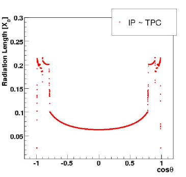
Figure 3.2: The amount of material up to the EM calorimeter in terms of radiation lengths as a function of $\cos\theta$

Materials in terms of nuclear interaction lengths are shown in Figure 3.3. The total is about 0.02 to 0.05 except at $\cos\theta=0$ where TPC central membrane has about 2.8 $\lambda$ contribution.

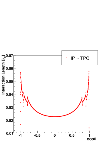
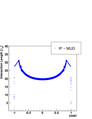
(A)	(B)

Figure 3.3: The amount of material in front of EM calorimeter in terms of nuclear interaction length (A) and to the end of Muon detector (B) as a function of $\cos\theta$

The momentum resolution for muons produced at $90^{\circ}$ is shown in Figure 3.4(A) for the cases of TPC only, TPC and IT, and TPC, IT and VTX combined [58]. To avoid particles hitting the TPC central membrane, particles are generated from a point slightly away from IP in Z direction. By combining TPC, IT and VTX, $\Delta p_{t}/p_{t}\sim 4\times 10^{-5}$ is achieved for 100 GeV muons.

Figure 3.4(B) shows the impact parameter resolution as a function of $p_{t}$ for different VTX detector configurations. The impact parameter is defined as a closest distance of tracks to the IP in the plane perpendicular to the Z axis. The cyan curve shows the performance in the case of the standard configuration. For the configuration shown by the blue curve, the inner radius of the innermost VTX layer is 1.7 cm, those of 5th and 6th layers are same as the standard, and that of 3rd and 4th layers are adjusted so that to have equal distance between 2nd and 3rd, and 4th and 5th layers. In the case of the purple curve, the inner radius of 1st layer is move to 2.4cm, while radius of remaining layers are adjusted similar to the blue curve case.

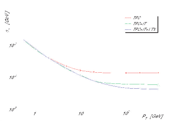
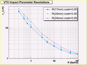
(A)	(B)

Figure 3.4: Momentum resolution(A) and impact parameter resolution of GLD as a function of Pt. Studied using a track generated at $90^{\circ}$ from IP by JUPITER.

The energy resolutions of the EM and HD calorimeters are shown in Figure 3.5 as a function of particle energies. In the study of the energy resolution of EM calorimeter, the range cut value for the Geant4 simulation was 10 $\mu m$, instead of default 1mm. This was necessary to obtain the energy resolution consistent with the beam test results. The energy resolution of the hadron calorimeter is show in Figure 3.5B, together with the beam test result with similar configuration. It is well known that results of the hadron shower program in Geant4 depends on the physics list. We compared models such as QGSP, LHEP and Jupiter physics lists (J4PhysicsList), but none of them reproduced the beam data resolution at high energies. In the Jupiter simulation, the Jupiter physics list derived from a Geant4 novice example is used as a default.

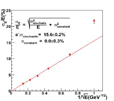
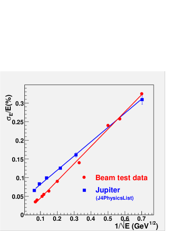
(A)	(B)

Figure 3.5: Energy resolution of EM (A) and HD(B) Calorimeter. Resolutions obtained by Jupiter simulation are compared with the beam test result in Figure (B)

3.3 Jet Energy Resolution

To achieve good resolution for jet energy measurements particle flow analysis (PFA) is crucial. In the PFA analysis, energies of charged particles are measured by trackers and neutral particle energies are measured by the calorimeter system. Since the calorimeter is sensitive to charged particles, removal of charged particle energy depositions in the calorimeter is essential. We used two methods for the PFA, cheated method [59] and realistic method [61], which will be discussed in the following subsections.

3.3.1 Resolution by cheated PFA

In the cheated method, cluster reconstruction and linking of charged track and calorimeter cluster for removal of charged track signals is pursued based on the Monte Carlo information. This gives optimistic estimates of the jet energy resolution, but still includes effects such as shower fluctuation in calorimeter, signal overlaps in readout cells of calorimeter, particle decays in tracker, etc.

In this study, we generated $e^{+}e^{-}\rightarrow q\bar{q}$ events at center of mass energies of 91.17 GeV, 350 GeV and 500 GeV. Only $u$, $d$, $s$ quarks were generated by Pythia [63] without initial state radiation. Generated events were simulated by JUPITER and reconstructed by the SATELLITES analysis modules . In this analysis charged particles measured by the TPC were fitted and connected to IT and VTX hits by the Kalman track fitter to make a combined track parameter, called hybrid track parameter. Hit points of candidate tracks were selected based on the Monte Carlo truth information.

In the JUPITER simulation, we kept an ID of tracks at the exit of the TPC sensitive volume and the ID is attached to each Calorimeter cells. This ID information was used to form a calorimeter cluster. If a track with the same ID is found in the TPC, the cluster in the calorimeter is deleted. If a track kinks in the TPC sensitive volume, we are left with a track before the kink (kink mother), a track after the kink (kink daughter) with a connected neutral cluster in the calorimeter, and the neutral cluster(neutral daughter) which might be produced at the kink. In this case, we used the track information of the kink mother and the neutral daughters for the PFO(kink mother scheme), instead of using the kink daughter and neutral daughters(kink daughter scheme). The kink mother scheme double counts the energies of neutral daughters, but the energy resolution was about 3% better than the link daughter scheme according to our study.

The jet energy resolution obtained by the cheated PFA algorithm is shown in Figure 3.6. In this study, we selected events where quarks were produced in the range $|\cos\theta_{q}|<0.8$. The invariant mass of the sum of all particle flow objects is plotted in the Figure. The curves shown in the figure are gaussian fits in the two $\sigma$ range from mean values. Fits were repeated until the conversion of $\sigma$.

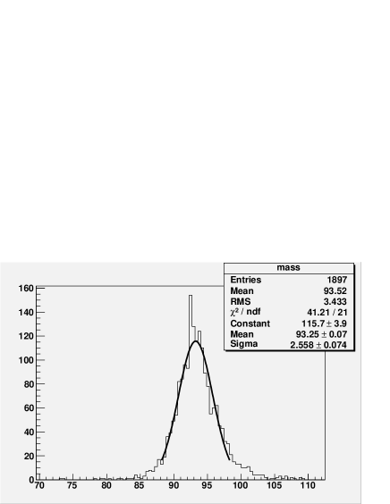
(A)
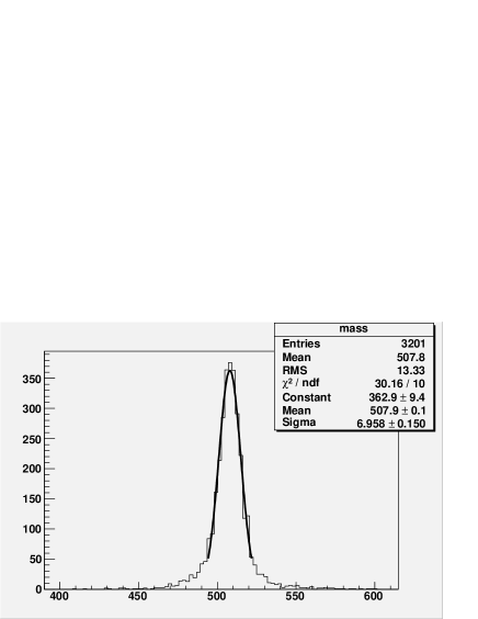
(B)	(C)

Figure 3.6: The reconstructed jet energy distribution of the process, $e^{+}e^{-}\rightarrow u\bar{u}$, $d\bar{d}$, or $s\bar{s}$ at $\sqrt{s}=91.17$(A), $300$(B), and $500$ GeV(C), respectively.

The widths of the jet energy distribution obtained from the fits are summarized in the Table.3.2. As seen in the table, the energy resolution for jets at the Z pole is about $26\%/\sqrt{E}$ and worsens slightly to about $30\%/\sqrt{E}$ at 500 GeV. In the table, the resolution for the case of QuickSim are shown in the same table for comparison. For QuickSim, we prepared two parameter sets, the good one for performance similar to the cheated PFA performance and the bad one corresponding to the realistic PFA resolution which will be discussed in the next subsection. The performance by the cheated PFA is the ultimate jet energy resolution with the current detector configuration which could be achieved by a clever PFA algorithm. The performance of the realistic PFA is limited by the performance of the PFA algorithm which will be improved in future developments. Final performance would be somewhere between two performances, thus, we will prepared two sets of QuickSim parameters to give optimistic and pessimistic estimates of physics performances.

Table 3.2: Summary of the jet energy resolution by the cheated PFA method of the process shown in Figure 3.6. 4th and 5th column shows the $\sigma$ in the case of QuickSim for good and bad parameter sets, respectively.

	Cheated PFA		Realistic PFA		QuickSim
$\sqrt{s}$(GeV)	$\sigma_{E}$ (GeV)	${\sigma_{E}\over\sqrt{E}}(\%)$	$\sigma_{E}$ (GeV)	${\sigma_{E}\over\sqrt{E}}(\%)$	$\sigma_{good}$(GeV)	$\sigma_{bad}$(GeV)
91.2	$2.56\pm 0.07$	$26.5\pm 0.7$	$3.65\pm 0.07$	$38.4\pm 0.7$	$2.35\pm 0.04$	$3.30\pm 0.05$
350	$5.66\pm 0.10$	$30.0\pm 0.5$	-	-	$5.75\pm 0.09$	$8.75\pm 0.14$
500	$6.96\pm 0.15$	$30.9\pm 0.7$	$19.8\pm 0.65$	$88.7\pm 2.9$	$7.21\pm 0.11$	$10.62\pm 0.17$

Factors which affect the performance of the cheated PFA are summarized in Table.3.3. In the table, the neutrino column shows the contribution of undetected-neutrino energies to the resolution of jet energies. The angle cut column shows those due to particles produced within 200 mrad from the beam pipe, and the $p_{t}$ cut column shows those due to particles with $p_{t}$ less than 230 MeV. These contributions were studied based on generator data of Z pole events. In the GLD, particles with $p_{t}$ less than 230 MeV is not reconstructed by TPC. If this cut off is reduced to 100 MeV by utilizing the track finding by IT, the contribution to the jet mass resolution from $p_{t}$ cut off is reduced to 0.4 GeV. On the other hand, it increases to 1.2 GeV, if a 5 Tesla solenoid field is used instead of 3 Tesla and only TPC track finder is used. Major contributions to the jet energy resolution are those by a fluctuation of measurement energies in EM Calorimeter and Hadron Calorimeter, which are indicated by EM CAL and HD CAL in the Table.3.3. These contributions were estimated by using particle energies at the entrance of the calorimeter, instead of energies measured by the scintillators.

Table 3.3: Breakdown of factors which affect the jet energy resolution. The meanings of each column are described in the text

Items	Total	neutrino	$p_{t}$ cut	angle cut	EM CAL	HD CAL	TPC
$\sigma$(GeV)	2.48	0.30	0.83	0.62	1.36	1.70	0.0

3.3.2 Realistic PFA

The GLD-PFA mainly consists of three parts: photon finding, charged hadron finding and neutral hadron finding. The photon finding is based on a calorimeter hit cluster. A small cluster is formed by the so called nearest-neighbor clustering method. Further clustering is performed by collecting the small clusters within a certain tube region. A cluster due to photon is then identified by using the cluster information such as longitudinal energy profile. Details of the photon finding can be found in [60]. After the photon finding, the charged hadron finding is performed. A charged track is extrapolated to the calorimeter, and distance between a calorimeter hit cell and the extrapolated track is calculated. The distance is calculated for any track/calorimeter cell combination. The calorimeter hit cells within a certain tube radius are connected to form a charged hadron cluster. Note that the tube radius for the ECAL and HCAL can be changed separately. Details of the charged hadron finding can be found in [61, 62]. After the charged hadron finding, the remaining calorimeter hits are classified into a hit due to a neutral hadron or a “satellite” hit due to a charged hadron. This is done by using a velocity and energy density information. The calculated velocity and energy density distribution can be found in Fig. 3.7.

Performance of the GLD-PFA is studied by using $Z\to q\bar{q}$ events at the center of mass energy of 91.2GeV. Note that the calorimeter configuration in the Jupiter is tower geometry and cell size for ECAL and HCAL is 4 cm $\times$ 4 cm and 12 cm $\times$ 12 cm, respectively. Performance of each tool described above is summarized in Table 3.4. The left most column shows a particle type identified by the GLD-PFA. The energy weighted efficiency ($E_{XXX}$) for the photon finding, charged hadron finding and neutral hadron finding are 85.2%, 84.4% and 60.5%, respectively. The energy weighted purity ($P_{XXX}$) for the photon finding, charged hadron finding and neutral hadron finding are 92.2%, 91.9% and 62.2%, respectively. Note that if satellites hits are included in the charged hadron, we gain 10% efficiency at a cost of 3% purity loss for the charged hadron finding. Figure 3.8 shows the energy sum for the Z pole events when the GLD-PFA is applied. 38%$/\sqrt{E}$ energy resolution is achieved by using the PFA while that of energy sum in the calorimeter is 60%$/\sqrt{E}$.

Table 3.4: Energy weighted efficiency ($E_{XXX}$) and purity ($P_{XXX}$) for each particle type identified by the GLD-PFA. CHD and NHD represents charged hadron and neutral hadron, respectively.

	$E_{Photon}$(%)	$E_{CHD}$(%)	$E_{NHD}$(%)	$P_{Photon}$(%)	$P_{CHD}$(%)	$P_{NHD}$(%)
Photon	85.2	0.626	8.19	92.2	2.03	5.11
CHD	4.59	84.4	16.4	1.67	91.9	3.44
NHD	6.27	4.51	60.5	11.2	24.1	62.2
Satellite	3.94	10.5	14.9	8.90	70.9	19.4
CHD + Satellite	8.53	94.9	31.3	2.67	89.0	5.64

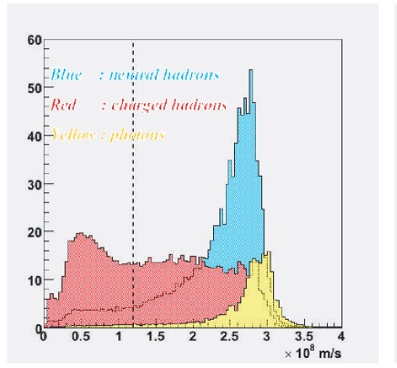
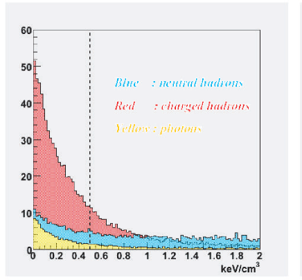
Figure 3.7: Velocity (left) and energy density (right) distribution for the remaining clusters. Current cut positions are indicated by the dotted line in the figures.

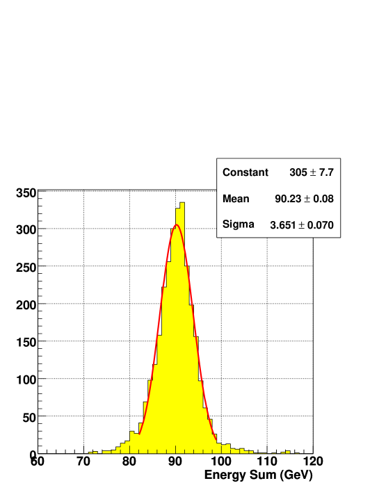
Figure 3.8: Energy sum for the Z pole events when the GLD-PFA is applied. 38%$/\sqrt{E}$ energy resolution is achieved by using the PFA.

3.4 Performance by physics benchmark process

3.4.1 $e^{+}e^{-}\rightarrow Zh$

The Higgsstrahlung ($e^{+}e^{-}\rightarrow Zh$) process which is one of the benchmark process is studied by using the QuickSim. Data equivalent to $500fb^{-1}$ have been generated for both signal and background processes ($e^{+}e^{-}\to ZZ,WW,$ and $e\nu W$). The center of mass energy ($E_{CM}$) and the Higgs mass ($M_{h}$) are set to be 350 GeV and 120 GeV, respectively. The remaining part of this section is subdivided according to the different final state of the Higgsstrahlung process. Events are generated by Pythia6.3[63] including beamstrahlung spectrum generated by the BSGEN package[55].

$\bullet~{}Zh\to\nu\bar{\nu}b\bar{b}$ and $Zh\to q\bar{q}b\bar{b}$

For $Zh\to\nu\bar{\nu}b\bar{b}$ mode, there are two jets in the final state. In the event selection, it is required that the missing mass calculated from the two jets is consistent with the $Z$ boson mass. It is also required that the visible energy ($E_{vis}$) is grater than 90 GeV and less than 200 GeV, and transverse momentum ($p_{t}$) is greater than 20 GeV/c. In addition to the above selection criteria, cut on number of off vertex track ($N_{\rm OffVertex}$) is imposed for b tag. The $N_{\rm OffVertex}$ is required to be greater than 6. For $Zh\to q\bar{q}b\bar{b}$ mode, there are four jets in the final state and therefore six jet-pair combinations are exist in an event. In order to select a correct jet pairing, both invariant mass of a jet-pair and missing mass calculated from the other jet-pair are required to be consistent with the $Z$ boson mass. The event thrust is also calculated and required to be less than 0.9. In addition, $E_{vis}>240$GeV and $N_{\rm OffVertex}>6$ are imposed in the 4-jet event selection. The distribution of invariant mass of two jets which are considered to come from the Higgs decay is shown in Fig. 3.9 after imposing all the above selection criteria. As described in the previous sections, current jet energy resolution is achieved to be $38\%/\sqrt{E}$ while the target resolution is $30\%/\sqrt{E}$. Two different parameter sets that reproduce $30\%/\sqrt{E}$ and $40\%/\sqrt{E}$ jet energy resolution are therefore prepared. Left (right) plot is for 2-jet (4-jet) event and top (bottom) plot is for jet energy resolution of $30\%/\sqrt{E}$ ($40\%/\sqrt{E}$). The blue area is signal events and gray area is all background events. In order to obtain accuracy for product of cross section ($\sigma$) and $h\to b\bar{b}$ branching ratio ($Br(h\to b\bar{b})$), the Higgs mass ($M_{h}$) and its accuracy ($\delta M_{h}$), the histograms are fitted by a combined function of the Lorenzian and exponential. The results are summarized in Table 3.5.

$\bullet~{}Zh\to l\bar{l}X$

For $Zh\to l\bar{l}X$ event selection, $e^{+}e^{-}$ pair or $\mu^{+}\mu^{-}$ pair is firstly identified. A particle whose energy deposit in the ECAL is consistent with that of the TPC is identified with an electron or positron. A charged particle which does not deposit energy in calorimeters in QuickSim is identified as a muon The invariant mass of the $e^{+}e^{-}$ pair and $\mu^{+}\mu-$ pair ($M_{Z}$) is then calculated and required to be consistent with the Z boson mass. For $Zh\to l\bar{l}X$ mode, performances between different beam condition and between different TPC spatial resolution are compared. The recoil mass distributions from the di-lepton pair after imposing all selection criteria for different beam condition and different TPC spatial resolution are shown in Figure 3.10 and Figure 3.11, respectively. Each selection criteria together with the number of signal events after imposing the cut and efficiency of the cut is summarized in Table 3.6 and Table 3.7. Note that $cos\theta_{i}$ is dip angle of an $i-th$ lepton. The histograms are fitted by the convoluted function of gaussian and the one inspired from the bremsstrahlung spectrum defined as follows;

$$F(m)=N_{H}\int F_{H}(m,t)e^{-\frac{t^{2}}{2\sigma^{2}}}dt+F_{Z}(m)$$

where $F_{H}(m,t)=\left(\frac{m+t-M_{h}}{\sqrt{s}-M_{h}}\right)^{\beta-1}$. In the case of bremsstrahlung spectrum, $\beta=\frac{2\alpha}{2\pi\log{\sqrt{s}/m_{e}}-1}$. When fitting spectrums including beamstrahlung effects, $\beta$ is determined by fits. $\alpha$ is fine structure constant and $m_{e}$ is the electron mass. $N_{H}$ is a normalization factor for signal events. The $F_{Z}(m)$ is a sum of an exponential function and a constant multiplied by a normalization factor, whose parameters are determined by fitting the background spectrum in the fit range.

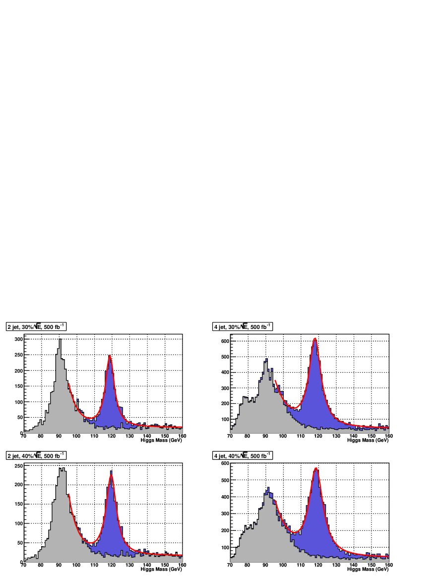
Figure 3.9: Higgs mass distribution for 2-jet (left) and 4-jet (right) in the final state. Top (bottom) plot is for jet energy resolution of $30\%/\sqrt{E}$ ($40\%/\sqrt{E}$).

Table 3.5: Summary of expected performance for 2-jet and 4-jet mode with different parameter set ($30\%/\sqrt{E}$ and $40\%/\sqrt{E}$). Kinematical constraint is not included yet.

Mode	$\nu\bar{\nu}b\bar{b}$		$q\bar{q}b\bar{b}$
Jet Energy Resolution	$30\%/\sqrt{E}$	$40\%/\sqrt{E}$	$30\%/\sqrt{E}$	$40\%/\sqrt{E}$
$\delta(\sigma\times Br(h\to b\bar{b}))$	2.74%	2.85%	1.59%	1.67%
$M_{h}$ (GeV)	118.7	119.5	117.9	118.5
$\delta M_{h}$ (MeV)	109.2	127.7	87.7	103.6

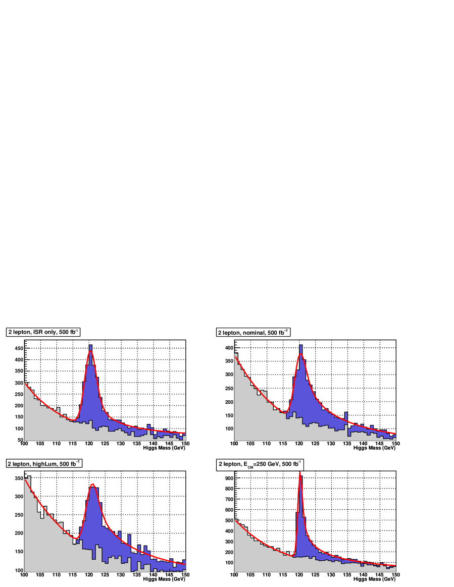
Figure 3.10: Comparison of higgs mass distribution between different machine parameters. The upper left, upper right, bottom left and bottom right histogram show the case of ISR only, nominal, highLum , respectively at $E_{CM}=350$ GeV. The right left histogram shows the case of nominal spectrum at $E_{CM}$=250 GeV. Notice that cut value for visible energy ($E_{vis}$) is 150 GeV for $E_{CM}$=250 GeV case.

Table 3.6: Breakdown of efficiency for each selection criteria together with an expected accuracy for the Higgsstrahlung cross-section ($\delta\sigma$) with and without b-tag, the Higgs mass width ($M_{h}$) and accuracy for the Higgs mass width ($\delta M_{h}$) for different machine parameters.

Machine Parameter	ISR only	Nominal	HighLum	$E_{CM}=250$ GeV
No Cut	3299 (1.0000)	3339 (1.0000)	3170 (1.0000)	4319 (1.0000)
$80.<M_{Z}<100.$ GeV	2889 (0.8757)	2907 (0.8706)	2755 (0.8691)	3745 (0.8671)
$|\cos\theta_{1,2}|<0.9$	2571 (0.8899)	2528 (0.8696)	2415 (0.8766)	3073 (0.8206)
$E_{vis}>250.$ GeV	2450 (0.9529)	2411 (0.9537)	2316 (0.9590)	3032 (0.9867)
$N_{OffVertex}>4.$	1552 (0.6335)	1524 (0.6321)	1459 (0.6300)	1876 (0.6187)
Total Efficiency	0.4704 $\pm$ 0.0087	0.4564 $\pm$ 0.0086	0.4603 $\pm$ 0.0089	0.4344 $\pm$ 0.0075
$\delta\sigma$	2.86%	2.88%	2.94%	2.57%
$\delta(\sigma\times Br(h\to b\bar{b}))$	3.03%	3.15%	3.35%	2.74%
$M_{h}$ (GeV)	120.0	119.5	119.9	120.0
$\delta M_{h}$ (MeV)	79.6	109.4	163.8	27.1

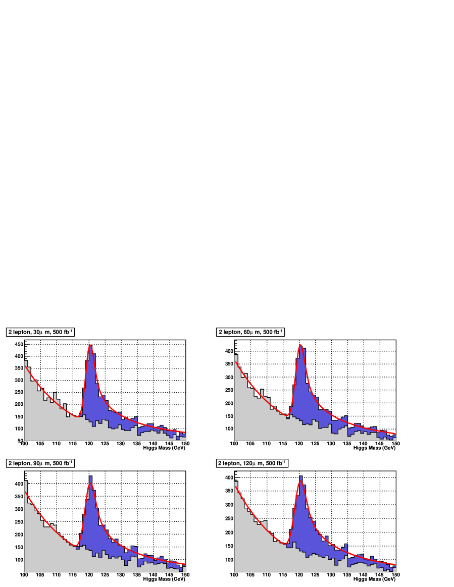
Figure 3.11: Comparison of higgs mass distribution between different TPC point resolution. The upper left, upper right, bottom left and bottom right histogram show the case of $30\mu m$, $60\mu m$, $90\mu m$ and $120\mu m$, respectively. Notice that default resolution is $150\mu m$.

Table 3.7: Breakdown of efficiency for each selection criteria together with an expected accuracy for the Higgsstrahlung cross-section ($\delta\sigma$) with and without b-tag, the Higgs mass width ($M_{h}$ ) and accuracy for the Higgs mass width ($M_{h}$) for different TPC point resolution.

TPC point resolution	30 $\mu m$	60 $\mu m$	90 $\mu m$	120 $\mu m$
No Cut	3382 (1.0000)	3375 (1.0000)	3361 (1.0000)	3349 (1.0000)
$80.<M_{Z}<100.$ GeV	2942 (0.8699)	2932 (0.8687)	2920 (0.8688)	2915 (0.8704)
$|\cos\theta_{1,2}|<0.9$	2540 (0.8634)	2538 (0.8656)	2533 (0.8675)	2530 (0.8679)
$E_{vis}>250.$ GeV	2422 (0.9535)	2421 (0.9539)	2417 (0.9542)	2414 (0.9542)
$N_{OffVertex}>4.$	1533 (0.6329)	1531 (0.6324)	1526 (0.6314)	1526 (0.6321)
Total Efficiency	0.4533 $\pm$ 0.0086	0.4536 $\pm$ 0.0086	0.4540 $\pm$ 0.0086	0.4557 $\pm$ 0.0086
$\delta\sigma$	2.87%	2.87%	2.88%	2.88%
$\delta(\sigma\times Br(h\to b\bar{b}))$	3.14%	3.14%	3.15%	3.15%
$M_{h}$ (GeV)	119.7	119.7	119.6	119.5
$\delta M_{h}$ (MeV)	77.7	86.3	96.4	105.0

Beam parameters compared in Figures 3.10 and 3.11 and Tables 3.6 and 3.7 are the case without the beamstrahlung effect ( ISR only), with the ”Nominal” pararameter and ”HighLum” parameter at $E_{CM}=350$ GeV, and the ”Nominal” parameter case at $E_{CM}=250$ GeV. Beamstrahlung spectrum ”Nominal”and ”HighLum” at 350 GeV and 250 GeV are calculated by the program, CAIN, using the parameters defined in ref.[6], except the center of mass energy. The difference of the specific luminosity at different energy is not considered and all results based on the integrated luminosity of 500 fb^-1. The width of Higgs distribution at 350 GeV in Table 3.6 and Figure 3.10 show that the beamstralung effect increase the width significantly, but it is small at 250 GeV thanks to the higher cross section and better momentum resolution due to lower lepton energies near threshold.

3.4.2 Vertex Charge Reconstruction

Quark charge sign selection is an essential tool for a number of physics analyses allowing e.g. the unfolding of cross-sections, measurement of spin correlations or angular analysis [64]. It is among the benchmarks for vertex detector performance [65]. For $b$-flavour jets, the sign of quark charge for the 40% of jets can be obtained by reconstructing the vertex charge, i.e. the sum of the charges of all tracks assigned to the $B$-hadron decay chain, as described in detail elsewhere [66]. Depending on all tracks in the decay chain being correctly distinguished from $IP$ tracks, an efficiency of vertex charge reconstruction is sensitive to the radius of the inner vertex detector layer and to multiple scattering effects [67].

Vertex charge reconstruction was studied using jets from $e^{+}e^{-}\rightarrow b\bar{b}$ events generated using the fast simulation SGV [68], interfaced to PYTHIA version 6.1.52 [69]. The vertex finder ZVTOP [70] was run on all tracks assigned to a jet by the JADE algorithm [71].

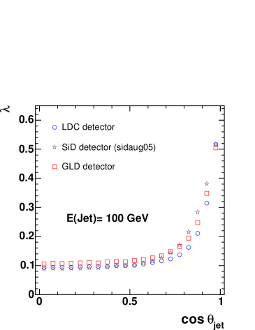
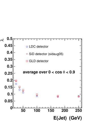
Figure 3.12: Comparison of the current vertex detector designs of the LDC, SiD and GLD concept studies in terms of the probability for reconstructing a neutral $B$ decay vertex as charged. The left figure shows the polar angle dependence for $50\,\mathrm{GeV}$ jets, and the right figure the energy dependence obtained when averaging over the polar angle range $0<|\mathrm{cos}\,\theta|<0.9$.

The performance of the GLD baseline vertex detector in terms of vertex charge reconstruction was studied as function of polar angle and jet energy. The leakage rate $\lambda$, defined as probability of reconstructing a neutral $B$ hadron as charged, was used to characterise detector performance. Figure 3.12 shows the angular and jet energy dependence for the GLD vertex detector compared to the vertex detectors of the SiD and LDC concept studies. All three vertex detectors were embedded in the same ’global detector geometry’, corresponding to the TESLA detector design [3]. At a jet energy of $50\,\mathrm{GeV}$, typical in multi-jet processes at the ILC, one finds a leakage rate of $\lambda\approx 10\,\%$ in the central region of the detector, degrading to $25\,\%$ for $0.85<|\mathrm{cos}\,\theta|<0.9$ due to increased lever arm from the IP and multiple scattering effects. When averaging over $0<|\mathrm{cos}\,\theta|<0.9$, values range from $\lambda\approx 8\,\%$ at the highest jet energy considered, $E_{\mathrm{jet}}=250\,\mathrm{GeV}$, to $\approx 20\,\%$ for $25\,\mathrm{GeV}$ jets. Those low energy jets contain more low-momentum tracks, which are more easily lost from the $B$ decay chain; also those jets are broader and hence more often contain tracks outside the angular acceptance of the detector.

Compared to the LDC vertex detector the current GLD detector design performs less well. The main reason for this is the larger inner layer radius of the GLD detector, which is needed because of its lower $B$ field of $3\,\mathrm{T}$. Performance of the GLD and the SiD, averaged over polar angle, is similar, with the GLD being worse than the SiD in the central region due to its larger radius, but better as one moves to the detector edge, where SiD performance is given by measurements in the vertex detector disks, which is impaired by the amount of material at the end of the short SiD barrel staves. While this study clearly shows some trends that ought to be taken into account in the further design, it should be noted that it is currently based on a fast simulation, and that differences between the global detectors were not considered. Furthermore, the differences are important only for events with high jet multiplicity. For two-jet processes such as $e^{+}e^{-}\rightarrow b\bar{b}$ at high energy, the measurement of vertex charge is insensitive to the different vertex detector options.

Acknowledgements

This work is supported in part by the following organizations and programs: Japan Society for the Promotion of Science (JSPS); JSPS-CAS-KOSEF Multilateral Cooperative program under the Core University Program; JSPS Japanese-German Cooerative Program; Japan-US Cooperative Program in High Energy Physics; Grant-in-Aid for Scientific Research No.17540282 from JSPS; Grant-in-Aid for Scientific Research No.17043010 from Ministry of Education and Science in Japan; U.S. Department of Energy; Deutsches Elektronen Synchrotron, Hamburg; Max-Planck-Institut fuer Physik, Munich; International Cooperative Research Program; Basic Atomic Energy Research Institute Program and the CHEP SRC program of the Korean Science and Engineering Foundation.

Bibliography

- [1]
- [2] K. Abe, et al., “Particle Physics Experiments at JLC”, KEK-Report-2001-11, hep-ph/0109166 (2001).
- [3] ”TESLA Technical Design Report”, DESY 2001-011, ECFA 2001-209, March 2001.
- [4] T. Abe, et al., “Linear Collider Physics Resource Book for Snowmass 2001”, BNL-52627, CLNS01/1279, FERMILAB-Pub-01/058-E, LBNL-47813, SLAC-R-570, UCRL-ID-143810-DR (2001).
- [5] J. Brau, et al., “Linear Collider Detector R&D”, Proceedings of LCWS2002 at Jeju, Korea, p.787.
-
[6]
T. Raubenheimer, “Suggested ILC Beam Parameter Range”,
http://www-project.slac.stanford.edu/ilc/acceldev/beamparameters.html - [7] Y. Sugimoto, talk at LCWS2005, Stanford, Mar. 2005.
- [8] Y. Giomataris, et al., ”Micromegas: A High Granularity Position Sensitive Gaseous Detector for High Particle Flux Environments”, Nucl. Instr. and Meth. A376 (1996) 29.
- [9] F. Sauli, ”GEM: A New Concept for Electron Amplification in Gas Detectors”, Nucl. Instr. and Meth. A386 (1997) 531.
- [10] J.L. Hewett, “Indirect Collider Signals for Extra Dimensions”, Phys. Rev. Lett. 82 (1999) 4765.
- [11] Y. Sugimoto, “Fine Pixel CCD Option for the ILC Vertex Detector”, talk at LCWS2005 at Stanford.
- [12] Y. Sugimoto and T. Nagamine, “Fine Pixel CCD R&D in Japan”, talk at Snowmass Workshop, 2005.
-
[13]
A. Seryi, “Discussion of ILC high luminosity parameters”,
http://www-project.slac.stanford.edu/lc/bdir/Meetings/beamdelivery/2005-07-26/
high_lumi_pars.ppt - [14] ATLAS Pixel Detector Technical Design Report, CERN/LHCC 98-13.
- [15] G. Lutz, “Semiconductor radiation detectors” New York: Springer-Verlag, 1999,
- [16] Hamamatsu Photonics, K.K. 1126-Ichino Cho, Hamamatsu City, Japan.
- [17] A.S. Schwarz, “Silicon strip vertex detectors at LEP”, Nucl. Instr. and Meth. A342, 218, 1994.
- [18] Electronic and Telecommunications Research Institute, Gajeong-Dong, Yuseong-gu, Daejeon, Korea.
- [19] Bruce A. Schumm, ”General Thoughts about Tracking for a Linear Collider Detector”, physics/0511038.
- [20] http://gdd.web.cern.ch/GDD/
- [21] LC-DET-2002-001, (LC Note available at http://www-flc.desy.de/lcnotes). See also http://mppmu.mpg.de/settles/tpc/prc for developments.
- [22] http://www.eudet.org/
- [23] http://www.physics.carleton.ca/research/ilc/tpc.html
- [24] M. Campbell, et al., ”Detection of single electrons by means of a Micromegas-covered MediPix2 pixel CMOS readout circuit”, Nucl. Instr. and Meth. A540 (2005) 295-304.
-
[25]
A. Bamberger, et al., ”Pixel Readout of GEMs”,
presentation by K. Desch at ECFA Linear Collider Workshop,
Vienna, Nov. 2005.
https://ilcsupport.desy.de/cdsagenda/fullAgenda.php?ida=a0575 - [26] M. Chefdeville, et al., ”An electron-multiplying ‘Micromegas’ grid made in silicon wafer post-processing technology”, Nucl. Instr. and Meth. A556 (2006) 490-494.
- [27] http://www.star.bnl.gov/
-
[28]
See http://alephwww.cern.ch for general information and
http://wisconsin.cern.ch/wiedenma/TPC/Distortions/CERN_LC.pdf - [29] R. Settles and W. Wiedenmann, LC Note in preparation.
-
[30]
America
Carleton U, U Cornell, Indiana U, LBNL, MIT, U Montreal, Purdue U, U Victoria, Yale U
Asia
Tsinghua U, XCDC: Hiroshima U, Minadamo SU-IIT, Kinki U, U Osaka, Saga U, Tokyo UAT, U Tokyo, Kogakuin U Tokyo, KEK Tsukuba, U Tsukuba
Europe
RWTH Aachen, CERN, DESY, U Hamburg, U Karlsruhe, UMM Kraków, MPI-Munich, NIKHEF, BINP Novosibirsk, LAL Orsay, IPN Orsay, U Rostock, CEA Saclay, PNPI StPetersburg, U Siegen - [31] TDR for the STAR TPC[27] (unpublished).
- [32] W. Wiedenmann, ”Alignment of the Aleph Tracking Devices”, 1992 Wire Chamber Conference, Vienna, 17-21 February 1992.
- [33] R. Settles, ”Backgrounds-in-the-detector Session”, Extended Joint Ecfa/Desy LC Workshop at St.Malo, France, 12-15 April 2002.
- [34] T. Suzuki, et al., Nucl. Instr. and Meth. A432 (1999) 48.
- [35] S. Uozumi, et al., Nucl. Instr. and Meth. A487 (2002) 291.
- [36] A. Nagano, et al., Nucl. Instr. and Meth. A557 (2006) 460.
- [37] T. Tauchi, K. Yokoya and P. Chen, Particle Accelerators 41 (1993) 29.
- [38] T. Tauchi and K. Yokoya, Phys. Rev. E 51 (1995) 6119.
- [39] P. Bambade, et al., hep-ph/0406010.
- [40] C.L. Bennett, et al., Astrophys. J. Suppl. 148 (2003) 1.
- [41] T. Tauchi, talk given at the second ACFA workshop on Linear Collider, 1999, Seoul, Korea.
-
[42]
A. Seryi, ”BDS Considerations”. presented at the Snowmass ILC Workshop 2005, Snowmass, CO, USA (2005), ILCAW0805,
http://www-conf.slac.stanford.edu/snowmass05/proceedings/proceedings.html -
[43]
Y. Sugimoto and T. Tauchi, ”VTX for GLD, Detector Magnet Field B and Machine Parameter Dependence
of RVTX”, ALCPG1413
( http://www-conf.slac.stanford.edu/snowmass05/proceedings/proc/papers/ALCPG1413.PDF ), proceedings of 2005 ALCPG & ILC Workshop, Snowmass, USA, August 14-27, 2005. - [44] A. Drozhdin, ”STRUCT Modeling of Collimation and Extraction System Performance”, presentation at the BDIR05 workshop, 21 June 2005, RHUL, UK.
- [45] K. Tanabe and T. Abe, the home URL is http://hep.phys.s.u-tokyo.ac.jp/lc/LCindex.html. Specific geometries can be seen in p.234 of ref.[48].
-
[46]
Beam deliver section in the BCD can be found at,
http://www.linearcollider.org/wiki/doku.php?id=bcd:beam_delivery:beam_delivery_home . - [47] N.V. Mokhov, ”MARS Modeling of Energy Deposition and Backgrounds in ILC BDIR”, presentation at the BDIR05 workshop, 21 June 2005, RHUL, UK.
- [48] ”GLC Project”, KEK Report 2003-7, see also http://lcdev.kek.jp/ProjReport/
- [49] T. Kawakubo, et al., ”Permanent Magnet Generating High and Variable Septum Magnetic Field and Its Deterioration by Radiation” , in proceedings of EPAC 2004, Lucerne, Switzerland, http://accelconf.web.cern.ch/AccelConf/e04/DEFAULT.HTM
- [50] T. Mihara, ”Development of Final Focus Permanent Magnet”, in proceedings of NANOBEAM 2005, KEK Proceedings 2005-20.
- [51] B. Parker, A. Seryi, Phys. Rev. ST Accel. Beams 8, 041001 (2005)
- [52] A. Seryi, T. Maruyama, B. Parker, ”IR Optimization, DID and Anti-DID”, in proceedings of NANOBEAM 2005, KEK Proceedings 2005-20.
- [53] W. Kozanecki, ”Normalized Backgrounds in ILC Tracking Detectors”, presented at the Snowmass ILC Workshop 2005, Snowmass, CO, USA (2005), ILCAW0546 .
- [54] S. Agostinelli, et al., Nucl. Instr. and Meth. A 506(2003)250.
- [55] available from http://acfahep.kek.jp/subg/sim/simtools/index.html and links therein.
- [56] Rene Brun and Fons Rademakers, ”ROOT - An Object Oriented Data Analysis Framework”, Proceedings AIHENP’96 Workshop, Lausanne, Sep. 1996, Nucl. Inst. and Meth. A 389 (1997) 81-86. See also http://root.cern.ch/.
- [57] See http://www-jlc.kek.jp/subg/offl/kaltest/ and references therein.
- [58] Atsushi Yamaguchi, Master Thesis, Tsukuba University, 2006 ( in Japanese ).
- [59] S. Yamamoto, et al., in preparation.
-
[60]
T. Fujikawa, “Photon Finding Procedure for GLD-PFA”, Proceedings of 2005 ALCPG & ILC Workshops, Snowmass, U.S.A., available at
http://www-conf.slac.stanford.edu/snowmass05/proceedings/proc/papers/ALCPG1109.PDF -
[61]
T. Yoshioka, “Particle Flow Algorithm for GLD”, Proceedings of 2005 ALCPG & ILC Workshops, Snowmass, U.S.A.,
available at
http://www-conf.slac.stanford.edu/snowmass05/proceedings/proc/papers/ALCPG1102.PDF -
[62]
T. Yoshioka, “PFA Algorithm”, Proceedings of 2005 ALCPG & ILC Workshops, Snowmass, U.S.A.,
available at
http://www-conf.slac.stanford.edu/snowmass05/proceedings/proc/papers/ALCPG1711.PDF - [63] ”Pythia 6.3”, T. Sjöstrand, L.Lönnblad, S. Mrenna, P. Skands, hep-ph/0308153.
- [64] C.J.S. Damerell, “Vertex Detectors and the Linear Collider”, Proceedings of the International Conference on Linear Colliders, LCWS 2005, Stanford, 18-22 March 2005.
- [65] M. Battaglia, Benchmark Panel Report sent to WWS and detector concept contacts; to appear in the proceedings of the International Conference on Linear Colliders, LCWS 2005, Stanford, 18-22 March 2005.
- [66] S. Hillert on behalf of the LCFI coll., “Quark charge measurement with an ILC vertex detector”, Proceedings of the International Conference on Linear Colliders, LCWS 2005, Stanford, 18-22 March 2005.
-
[67]
S. Hillert, C.J.S. Damerell on behalf of the LCFI coll., “Physics
potential of vertex detector as function of beam pipe radius”,
Proceedings of 2005 ALCPG & ILC Workshops, Snowmass, U.S.A.,
available at
http://www-conf.slac.stanford.edu/snowmass05/proceedings/proc/papers/ALCPG1403.PDF - [68] available from http://berggren.home.cern.ch/berggren/sgv.html .
- [69] T. Sjöstrand, et al., Comp. Phys. Comm. 135 (2001) 238.
- [70] D.J. Jackson, Nucl. Instr. and Meth. A 388 (1997) 660.
- [71] JADE Coll., S. Bethke, et al., Phys. Lett. B 213 (1988) 235.