Magnetic domain-walls and the relaxation method

Abstract

The relaxation method used to solve boundary value problems is applied to study the variation of the magnetization orientation in several types of domain walls that occur in ferromagnetic materials. The algorithm is explained and applied to several cases: the Bloch wall in bulk magnetic systems, the radial wall in cylindrical wires and the Néel wall in thin films.

I Introduction

A domain is a region in a ferromagnetic material with the magnetization along a given direction. A magnetic material contains many domains with different magnetizations pointing in different directions in order to minimize the total magnetostatic energy. Regions with different orientations of their magnetization can be close to one another albeit with a boundary called a domain wall (containing typically about 10² – 10³ atoms).
Saturation occurs when all these regions align along some common direction imposed an external applied field, the total magnetization reaching its largest value $M_{s}$.
The width of a domain wall is equal to $\pi\sqrt{A/K}$ where $A$ is the typical nearest neighbor Heisenberg exchange interaction and $K$ the typical anisotropy constant (see Table 1). Hence, a magnetic wall results from exchange and anisotropy, being thinner for higher anisotropy or smaller exchange (In Fe it is about 30 nanometers whereas in a hard material like Nd₂Fe₁₄B it is about 5 nanometers, only). Domain wall energy is given by $4\sqrt{AK}$ illustrating once again the competing role of exchange and anisotropy.
For bulk materials, walls of the Bloch type occur whereas in thin films Néel type walls are encountered when the film thickness is close to the exchange length (defined by $\ell_{ex}=\sqrt{A/K}$, which is a few nanometers for ferromagnetic materials like Ni, Fe or Co, see Table 1). In the case of soft or amorphous materials characterised by a vanishing anisotropy constant $K$, one uses rather the magnetostatic exchange length defined by $\ell_{ex}=\sqrt{A/M_{s}^{2}}$. In all cases, the wall width $\delta$ is obtained from the exchange length via $\delta=\pi\ell_{ex}$.
A single parameter $Q=2K/M_{s}^{2}$ allows to discriminate between simple ($Q<1$) and complex wall profiles $(Q>1)$ (see Malozemoff and Slonczewski malo ). For example, in fig. 1 a Bloch wall, belonging to the class ($Q<1$) is depicted with the magnetization rotating in a vertical plane.
Mathematically, a domain wall appears as a result of a non-linear two-point boundary value problem (TPBVP) since it separates two distinct regions with a well defined value of the magnetization. The TPBVP originates from a minimization of the total magnetic energy that contains in general a competition between the anisotropy and exchange energies.
In this work, a general numerical approach based on the relaxation method is applied to the study of domain profiles in several geometries: bulk, wires and thin films.
This report is organised as follows: In section 2, the numerical relaxation method is described; in section 3 we discuss Bloch walls, whereas radial walls in cylindrical wires are described in section 4. In section 5 Néel walls are described and finally section 6 contains a discussion and a conclusion.

II The relaxation Method

Traditionally, TPBVP are typically tackled with the shooting method. The shooting method typically progresses from one boundary point to another using, for instance, Runga-Kutta integration recipes with a set of initial conditions attempting at reaching the end boundary.
For regular Ordinary Differential Equations (ODE), simple shooting is enough to reach the solution. In more complicated ODE, one has to rely on double shooting also called shooting to a fitting point. The algorithm consists of shooting from both boundaries to a middle point (fitting point) where continuity of the solution and derivative are required. In certain cases, one even has to perform multiple shooting in order to converge toward the solution stoer .
In the case of presence of singularities (within the domain or at the boundaries) the shooting method in all its versions: simple, double or multiple does not usually converge. We find that it is the case also with domain walls because of a rapid drop of the solution somewhere in the integration interval (due to the rapid change of the magnetization orientation in the wall). In this work, we develop, a new method to tackle the domain wall problem based on the relaxation method and find it quite suitable to handle relatively fast changes in the solution.

The basic idea of the relaxation method is to convert the differential equation into a finite difference equation (FDE). When the problem involves a system of $N$ coupled first-order ODE’s represented by FDE’s on a mesh of $M$ points, a solution consists of values for $N$ dependent functions given at each of the $M$ mesh points, that is $N\times M$ variables in all. The relaxation method determines the solution by starting with a guess and improving it, iteratively. The iteration scheme is very efficient since it is based on the multidimensional Newton’s method (see Numerical recipes recipes ). The matrix equation that must be solved, takes a special, block diagonal form, that can be inverted far more economically both in time and storage than would be possible for a general matrix of size $(MN)\times(MN)$. The solution is based on error functions for the boundary conditions and the interior points.
Given a set of $N$ first-order ODE’s depending on a single spatial variable $x$:

$$\frac{\bm{dy}_{j}}{dx}=\bm{g}_{j}(x,\bm{y}_{1},\dots,\bm{y}_{N}),j=1,2,\dots N$$ (1)

we approximate them by the algebraic set:

$$0=\bm{E}_{k}=\bm{y}_{k}-\bm{y}_{k-1}-(x_{k}-x_{k-1})\bm{g}_{k}(x_{k},x_{k-1},\bm{y}_{k},\bm{y}_{k-1}),k=2,3,\dots M$$ (2)

over a set of $M-1$ mesh points defining $[x_{k-1},x_{k}]$ intervals with $k=2,3,\dots M$.
The FDE $\bm{E}_{k}$ provide $N$ equations coupling $2N$ variables at the mesh points of indices $k-1,k$. The FDE’s provide a total of $M(N-1)$ equations for the $MN$ unknowns. The remaining equations come from the boundary conditions recipes :
At the first boundary $x_{1}$ we have: $0=\bm{E}_{1}=\bm{B}(x_{1},\bm{y}_{1})$
At the second boundary $x_{2}$, we have: $0=\bm{E}_{M+1}=\bm{C}(x_{M},\bm{y}_{M})$
The vectors $\bm{E}_{1}$ and $\bm{B}$ have $n_{1}$ non-zero components corresponding to the $n_{1}$ boundary conditions at $x_{1}$. The vectors $\bm{E}_{M+1}$ and $\bm{C}$ have $n_{2}$ non-zero components corresponding to the $n_{2}$ boundary conditions at $x_{2}$, with $n_{1}+n_{2}=N$ the total number of ODE’s.

The main idea of the relaxation method is to begin with initial guesses of $\bm{y}_{j}$ and relax them to the approximately true values by calculating the errors $\bm{E}_{i}$ to correct the value of $\bm{y}_{j}$ iteratively. Relaxation might be viewed as a rotation of the initial vector (representing the solution) under the constraints defined by $\bm{E}_{i}$. The evolution of the relaxation process, is obtained from solution-improving increments $\Delta\bm{y}_{k}$ that can be evaluated from a first-order Taylor expansion of the error functions $\bm{E}_{k}$.
It is that expansion that results in the matrix equation possessing a special block diagonal form, allowing inversion economically in terms of time and storage (see ref. recipes ).

III Bloch walls

The energy of an uniaxial ferromagnetic material comprises anisotropy and exchange terms. An infinite volume is considered to exclude any shape related demagnetization energy. Exchange energy density is given by landau :

$$\frac{A_{ik}}{2}(\frac{\partial M_{l}}{\partial x_{i}})(\frac{\partial M_{l}}{\partial x_{k}})$$ (3)

where Einstein summation convention is used for repeated indices $i,k,l=1...3$. The uniaxial anisotropy energy is given by $K_{ij}M_{i}M_{j}$ with $i,j=1...3$. For simplicity, we assume a single uniform exchange constant $A$ (see Table 1) and a sole dependence on the $x$ coordinate of all components of the magnetization $\bm{M}$. We have $\bm{M}=(0,M_{s}\sin\theta(x),M_{s}\cos\theta(x))$ (see fig. 1). $\theta(x)$, the angle the magnetization makes with the $z$ axis considered as the anisotropy axis. The sought profile is the function $\theta(x)$. $M_{s}$ is the saturation magnetization when all individual magnetic moments in the material are aligned along the same direction.

Integrating over all the volume, the total energy is given by:

$$E=\int_{-\infty}^{\infty}\{\frac{A}{2}{(\frac{\partial\bm{M}}{\partial x})}^{2}+\frac{K}{2}M_{y}^{2}\}dx$$ (4)

This can be rewritten as:

$$E=\frac{M_{s}^{2}}{2}\int_{-\infty}^{\infty}[A{(\frac{d\theta}{dx})}^{2}+K\sin^{2}\theta]dx$$ (5)

The energy minimum is found by nulling the variational derivative of $E$ with respect to $\theta$. We find:

$$\frac{d^{2}\theta}{dx^{2}}-\xi\sin\theta\cos\theta=0$$ (6)

with $\xi=\frac{K}{A}$. The Bloch wall profile is given by the solution to the above second-order ODE written as a system of two first-order equations:

$$\frac{dy_{1}}{dx} = y_{2}$$ (7)

$$\frac{dy_{2}}{dx} = \xi\sin\theta\cos y_{1}$$ (8)

where $y_{1}=\theta(x)$ satisfies the boundary conditions:

$$\lim_{x\rightarrow-\infty}y_{1}(x)=\pi;\hskip 28.45274pt\lim_{x\rightarrow\infty}y_{1}(x)=0$$ (9)

It is understood that the sharp transition between the $\theta=0$ phase and the $\theta=\pi$ is behind the failure of all shooting methods.

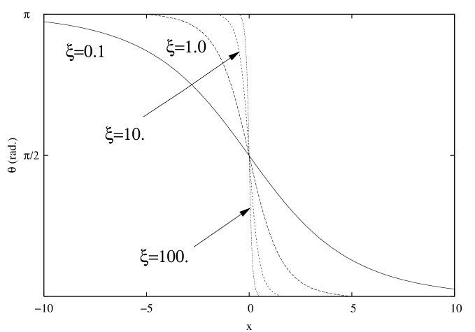
Figure 2: Variation of the magnetization angle with distance for a Bloch wall for various values of the exchange anisotropy ratio $\xi$. The analytical result $\theta(x)=2\tan^{-1}(e^{-x})$, for $\xi=1$, is indistinguishable from the relaxation method result.

Using the relaxation method, we easily obtain the wall profiles for any value of $\xi$ as displayed in fig. 2.

Actually, the Bloch wall problem is single scale and we can without performing the calculation for every $\xi$ value, do it for one value and then change the scale accordingly. This is done as follows: The width of the domain wall is given by $\delta=1/\sqrt{\xi}$ as explained previously. We perform a scaling transformation to the $x$ coordinate as: $\tilde{x}=x/\delta$ turning the ODE into:

$$\frac{d^{2}\theta}{d\tilde{x}^{2}}-\sin\theta\cos\theta=0$$ (10)

The exact analytical solution of the above equation given by: $\theta(\tilde{x})=2\tan^{-1}(e^{-\tilde{x}})$ is indistinguishable from the relaxation method results displayed in fig. 2.

Numerically, this means one can do the calculation for $\xi=1$ and later on rescale the $x$ variable in order to get the solution for any value (arbitrarily large or small) of $\xi$. Despite the power of the relaxation method, we noticed that when $\xi\leq 10^{-5}$ or when $\xi\geq 10^{4}$, convergence becomes difficult due to rounding and conditioning errors.

That rescaling works for many types of walls except Néel wall where we have an additional scale controlling the profile (see section V).

IV Radial walls

The energy density of an infinite cylindrical (see fig.3) uniaxial ferromagnetic material comprising uniaxial anisotropy and exchange terms is given by:

$$\frac{A}{2}[{(\frac{\partial\bm{M}}{\partial r})}^{2}+{(\frac{\partial\bm{M}}{r\partial\phi})}^{2}+{(\frac{\partial\bm{M}}{\partial z})}^{2}]$$ (11)

For simplicity, we assume a single uniform exchange constant $A$ and a sole dependence on the radial coordinate $r$ of all the magnetization components of $\bm{M}$. Integrating over all a cylindrical volume of radius $R$, the total energy is given by:

$$E=\frac{1}{\pi R^{2}}\int_{a/2}^{R}\{\frac{A}{2}[{(\frac{d\theta}{dr})}^{2}+\frac{\sin^{2}\theta}{r^{2}}]+K\cos^{2}\theta\}2\pi rdr$$ (12)

where $\theta$ is the angle the magnetization makes with the $z$ axis (see fig. 3). $a$ plays the role of a lattice parameter, the minimal core radius, regularising the integral (see for instance frei ). As in the Bloch wall case, we consider that $\theta$ is a function of one spatial coordinate only ($r$ in this case). Since the anisotropy energy is given by: $K\cos^{2}\theta$ with $K$ positive, the base plane (perpendicular to the $z$ axis) is easy, meaning the minimum of anisotropy energy is obtained when $\theta=\pi/2$ (see fig.3).

The total energy minimum is found by nulling the variational derivative of $E$ with respect to $\theta(r)$. We find:

$$\frac{d^{2}\theta}{dr^{2}}+\frac{1}{r}\frac{d\theta}{dr}+\frac{\sin 2\theta}{2}[\xi-\frac{1}{r^{2}}]=0$$ (13)

with $\xi=\frac{2K}{A}$. The radial wall profile is given by the solution to the above second-order ODE (equivalent to system of two first-order ODE’s like the Bloch case) with the boundary conditions:

$$\lim_{r\rightarrow a}\theta(r)=0;\hskip 28.45274pt\lim_{r\rightarrow R}\theta(r)=\pi/2$$ (14)

The limits: $a\rightarrow 0;R\rightarrow\infty$ are taken afterwards.

Using several values of $\xi$ we obtain the radial wall profile in fig.4. Again, like in the Bloch case, there is a single length involved and it suffices in fact to solve the TPBVP for a single case $\xi=1$ and rescale all variables accordingly. This is not the case of Néel walls as decribed in the next section.

V Néel walls

Néel realized that in a regime where the thickness of a ferromagnetic film becomes comparable to the Bloch wall width, a transition mode within the plane can lower the total energy decisively. Unlike the Bloch wall problem where only two energy components (exchange and anisotropy) exist balanced by a single length scale, the Néel wall problem incorporates two characteristic length scales. The new length arises from the competition with an additional energy component, the internal field energy. This has important physical, mathematical and numerical consequences. On the physical side, a very rich behaviour of Néel walls in thin films was shown recently in ref. garcia .
Domain structures in thin inhomogeneous ferromagnetic films with smooth and small inhomogeneities in the exchange and anisotropy parameters yield very complex domain structures garcia . Domain walls are fixed near certain inhomogeneities but do not repeat their spatial distribution. In addition there are metastable chaotic domain patterns in periodically inhomogeneous films.
The mathematical description of Néel walls entails the introduction of an internal magnetic field $\bm{H}$ created by $\rho$ the induced pole density induced by the rotation of $\bm{M}$. Mathematically we have div$\bm{H}$=-div$\bm{M}$=$\rho$. The magnetization is expressed as $\bm{M}=(M_{s}\sin\theta(x),M_{s}\cos\theta(x),0)$ in the $xyz$ coordinates defined in fig. 5. Since the divergence of $\bm{M}$ is not zero, we have an induced pole density $\rho$. In contrast, $\rho=0$ in the Bloch wall case since we recall in this case (see section III), $\bm{M}=(0,M_{s}\sin\theta(x),M_{s}\cos\theta(x)$). Assuming as done previously, that the components of $\bm{H}$ depend solely on the spatial variable $x$ (see fig. 5), we obtain:

$$\rho=-{\rm div}\bm{M}=-\frac{\partial M_{x}}{\partial x}=-M_{s}\frac{d(\sin\theta)}{dx}$$ (15)

The ODE that controls the wall profile $\theta(x)$ is derived exactly as before (taking account of the exchange and anisotropy terms) with the addition of the Zeeman term accounting for the presence of the internal field $H(x)$:

$$2A\frac{d^{2}\theta}{dx^{2}}-K\sin 2\theta+M_{s}H(x)\cos\theta=0$$ (16)

The uniaxial anisotropy term is $K\sin 2\theta$ with $\theta$, the angle the magnetization makes with the $y$ axis (the anisotropy axis).

Note that the demagnetization energy (due to the finite thickness of the film along the $z$ direction) is zero, since it is given by $2\pi N_{ij}M_{i}M_{j}$ with $N_{xx}=N_{yy}=0,N_{zz}=1$, and $M_{z}=0$.

The difference between this equation and the previous ones (Bloch and Radial cases) is that the internal field term $\bm{H}$ depends on the profile $\theta(x)$. Writing $H(x)$ instead of $H(\theta(x))$ makes the wall-profile equations non-autonomous because of the explicit $x$ dependence in $H(x)$. Additionally these equations are integro-differential because of the dependence of $H(x)$ on $\theta(x)$ (see for instance cervera ).
In this work we consider the thin film approximation and retrieve a system of three ODE’s by introducing a third function $y_{3}=H(x)/H_{K}$ with $H_{K}=2K/M_{s}$ the anisotropy field. The ODE system to solve is written with respect to normalised coordinates $\tilde{x}=x/\delta$ where $\delta$ is the wall thickness ($\delta=1/\sqrt{\xi}$ where, as before, $\xi=\frac{K}{A}$):

$$\frac{dy_{1}}{d\tilde{x}} = y_{2}$$ (17)

$$\frac{dy_{2}}{d\tilde{x}} = \sin y_{1}\cos y_{1}-y_{3}\cos y_{1}$$ (18)

$$\frac{dy_{3}}{d\tilde{x}} = -\pi Cy_{2}\cos y_{1}$$ (19)

The magnitude of the coupling constant $C=\frac{M_{s}}{\pi H_{K}}$ has a strong effect on the solution of the system. In the limit $C=0$ we recover the simple case with no internal field $H(x)=0$ like the Bloch wall case. As the magnitude of $C$ increases, we get a greater variation in the spatial dependence of $y_{3}(\tilde{x})$ and the system might become unstable and display numerical oscillations in spite of a drastic reduction of the integration step.

We convert the boundary conditions from the $]-\infty,+\infty[$ interval to the $[0,+\infty[$ interval:

$$\lim_{\tilde{x}\rightarrow 0}y_{1}(\tilde{x})=\pi/2;\hskip 28.45274pt\lim_{\tilde{x}\rightarrow\infty}y_{1}(\tilde{x})=0\hskip 28.45274pt\lim_{\tilde{x}\rightarrow\infty}y_{3}(\tilde{x})=0$$ (20)

We describe below a special algorithm, that we developed, based on the relaxation method coupled to an iterative procedure. The pseudo-code follows:

1. Initially, we introduce a guess profile (say $\theta_{0}(x)$), extract from it the pole density $\rho_{0}(x)$ using eq. 15 and determine from it the field derivative using the divergence equation: $\frac{dH(x)}{dx}=\rho(x)$.

2. The ODE system is solved and that allows us to extract a new profile (say $\theta_{1}(x)$) that yields a new pole density $\rho_{1}(x)$ (using eq. 15).

3. We repeat this procedure to the $n$-th step with a profile $\theta_{n}(x)$ yielding a pole density $\rho_{n+1}(x)$ that provides a profile $\theta_{n+1}(x)$. The procedure stops when the difference between the two profiles $\theta_{n}(x)$ and $\theta_{n+1}(x)$ in the mean-square sense becomes smaller than an error criterion.

The latter profile will have then relaxed self-consistently to the sought optimal profile that minimises the total energy (see ref. cervera and references within).

The results we obtain with various values of $C$ for $\theta(\tilde{x})$ and the internal field $H(\tilde{x})/H_{K}$ are displayed in fig. 7 and fig. 6. The analytical result obtained for $C=0$ (Bloch case), given by: $\theta(\tilde{x})=2\tan^{-1}(e^{-\tilde{x}})$ is displayed in fig. 6 and is indistinguishable from the numerical results we obtain with the relaxation method on the system 19.
The results obtained for the internal field displayed in fig. 7 show, as expected (see for instance ref. cervera ), that when $C$ increases, the field (absolute) amplitude becomes larger close to the origin. In addition, as $C$ increases the field extends to larger distances farther from the origin. That, in fact, points to the origin of the integro-differential nature of the problem. Inspection of eq. 16 shows that in addition to the usual length scale (wall width) $\delta=1/\sqrt{\xi}$, we have another length given by: $\delta_{N}=\sqrt{A/(KC)}=\delta/\sqrt{C}$ arising from the internal field whose strength is given by the coupling constant $C$. As $C$ increases, non-local effects increase, the length ratio $\delta_{N}/\delta=1/\sqrt{C}$ decreases (making the competition between the two lengths harder to deal with because of the disparity of the two lengths) and it becomes more and more difficult for the relaxation method to find an optimum result satisfying the TPBVP.

VI Discussion and Conclusion

The magnetic domain profile is a challenging mathematical and numerical problem. In this work, we treated with the relaxation method, in the simple domain structure case ($Q<1$), wall configurations in several interesting physical cases: Bloch walls in ferromagnetic bulk systems, radial walls in cylindrical ferromagnetic wires and the Neel walls in thin ferromagnetic films assuming in all cases uniaxial anisotropy.
In the Néel case, we showed than in the thin film approximation (in present technology, thin means $\sim 10-100\AA$) one is able to solve the wall problem with the relaxation method with a proper selection of the variables. Nevertheless, a major difficulty appears at higher value of the thickness $t$ along the $z$ direction (see fig. 5).
When the thickness of the film increases the system becomes a full integro-differential system whereas in the thin film approximation, we get a set of coupled non-linear ODE’s that we have to treat with a special self-consistent algorithm. The non-locality of the internal field is responsible for the appearance of logarithmic tails in the spatial variation of the magnetization angle. That means the TPBVP must be solved over an ever increasing interval size. The algorithm we have developed still applies but one has to use the finite thickness formulas for the field $H(x)$ (eq. 24) and its derivative $\frac{dH(x)}{dx}$ (eq. 25) as shown in the Appendix. The extension of this work to other types of walls (originating from other types of anisotropy for instance, or the complex wall shape case $Q>1$) or wall dynamics is challenging since the wall profile rapid change imposes a constraint on the time integration step.
Previously, Smith treated domain wall dynamics in small patterned magnetic soft thin ($\sim 100\mu$m) films and turned the dynamic Landau-Lifshitz equations into a set of coupled non-linear ODE’s. It turns out that the system of equations, he found is stiff (see for instance ref. ascher ), imposing a very small integration timestep slowing down considerably the integration process on top of the difficulties of the TPBVP.

The extension of this work to domain structures in inhomogeneous media (see ref. garcia ) is also quite interesting, particularly to the case of thin magnetic films that are of high technological interest such as recording, memories (Magnetic RAM’s and Tunnel Junctions) and Quantum computing and communication.

VII Acknowledgements

The authors wish to acknowledge friendly discussions with M. Cormier (Orsay) regarding dynamic effects in ferromagnetic materials and N. Bertram (San Diego) for sending some of his papers prior to publication.

APPENDIX

We derive, in this Appendix, the formula for the internal field from the induced pole density. The magnetization is expressed as $\bm{M}=(M_{s}\sin\theta(x),M_{s}\cos\theta(x),0)$ in the $xyz$ coordinates defined in fig. 5. Since the divergence of $\bm{M}$ is not zero, we have an induced pole density $\rho(x)$. The internal field is obtained from the pole density by integration accounting for the finite thickness of the film.
Using div$\bm{H}=-\rho$ we infer from general theorems of electromagnetism that:

$$\bm{H(r)}=-\frac{1}{4\pi}\int d\bm{r^{\prime}}\rho(\bm{r^{\prime}})\frac{(\bm{r-r^{\prime}})}{{|\bm{r-r^{\prime}}|}^{3}}$$ (21)

with $\bm{r}=(x,y,z),\bm{r^{\prime}}=(x^{\prime},y^{\prime},z^{\prime})$.
By symmetry we have $H_{y}=H_{z}=0$ and the $x$ component $H(x)$ in the plane $z=0$ is written as:

$$H(x)=-\frac{1}{4\pi}\int_{-\infty}^{+\infty}dx^{\prime}\int_{-\infty}^{+\infty}dy^{\prime}\int_{-t/2}^{t/2}dz^{\prime}\rho(x^{\prime})\frac{(x-x^{\prime})}{{[{(x-x^{\prime})}^{2}+{(y-y^{\prime})}^{2}+{(z^{\prime})}^{2}]}^{3/2}}$$ (22)

A first integration over $y^{\prime}$ gives:

$$H(x)=-\frac{1}{2\pi}\int_{-\infty}^{+\infty}dx^{\prime}\int_{-t/2}^{t/2}dz^{\prime}\rho(x^{\prime})\frac{(x-x^{\prime})}{[{(x-x^{\prime})}^{2}+{(z^{\prime})}^{2}]}$$ (23)

A second integration over $z^{\prime}$ yields the result:

$$H(x)=\frac{1}{\pi}\int_{-\infty}^{\infty}\rho(x^{\prime})\tan^{-1}[\frac{t}{2(x-x^{\prime})}]dx^{\prime}$$ (24)

The relation div$\bm{H}=\rho$ gives the integral expression of $\frac{dH(x)}{dx}$ needed in the integration of system of ODE’s eq. 19:

$$\frac{dH(x)}{dx}=\frac{2t}{\pi}\int_{-\infty}^{\infty}\rho(x^{\prime})\frac{1}{4{(x-x^{\prime})}^{2}+t^{2}}dx^{\prime}$$ (25)

In the finite thickness case, one needs the solve an integro-differential system of equations defined by the system of ODE’s 19 and the integral eq. 25. In the case of thin films $t\rightarrow 0$, we recover from eq. 25 the previous definition $\frac{dH(x)}{dx}=\rho(x)$ by using the $\delta$ function definition:

$$\delta(x-x^{\prime})=\frac{1}{\pi}\lim_{t\rightarrow 0}\frac{2t}{4{(x-x^{\prime})}^{2}+t^{2}}$$ (26)

TABLES AND FIGURES

Material	$T_{c}$	$\mu_{0}M_{s}$	$A$	$K$	$\ell_{ex}$
Unit	[K]	[T]	10-11[J/m]	105 [J/m3]	[nm]
Fe	1044	2.16	1.5	0.48	2.8
Co	1398	1.82	1.5	5	3.4
Ni	627	0.62	1.5	-0.057	9.9
Permalloy	720	1.0	1.3	0	5.7
CrO2	393	0.5	0.1	0.22	3.2
SmCo5	993	1.05	2.4	170	7.4

Table 1: Properties of Ferromagnetic Materials: $T_{c}$ is Curie temperature, $\mu_{0}$ is vacuum permeability, $M_{s}$ is saturation magnetization, $A$ is exchange constant, $K$ is magneto-crystalline anisotropy constant and $\ell_{ex}$ is exchange length. Note that in the case of Permalloy (Ni_xFe_100-x alloys with $x\sim 80$), one uses the magnetostatic exchange length defined as $\ell_{ex}=\sqrt{A/M_{s}^{2}}$ since $K\sim 0$.

Figure 1: Behaviour of the magnetization direction for a Bloch wall. For an arbitrary point along the $x$ axis, the magnetization $\bm{M}$ whose rotation is entirely confined within the vertical $zOy$ plane makes the angle $\theta$ with the vertical $z$ axis, the anisotropy axis.

Figure 3: Cylindrical coordinates displaying the spatial variation of the magnetization angle with radial distance from the wire axis. The base plane perpendicular to the wire axis $z$ is an easy plane.

Figure 4: Variation of the magnetization angle $\theta$ with radial distance $r$ from the wire axis for various values of the exchange anisotropy ratio $\xi$. As we increase $\xi$ the angle increases faster from 0 (Easy axis along $z$) to $\pi/2$ (Easy plane $\bot z$)

Figure 5: Variation of the magnetization angle with distance for a Néel wall in a thin film. The angular variation is in the $xOy$ plane. The film is of infinite dimensions along the $x$ and $y$ directions and a finite thickness $t$ along the $z$ direction. The anisotropy axis is along $y$.

Figure 6: Variation of the magnetization angle with distance for a Néel wall for various values of the coupling constant $C$. Uppermost curve is for $C=0$, whereas lower curves correspond respectively to $C$=1, 10, 50 and finally 100. The exact result corresponding to zero thickness along the $z$ direction is indistinguishable from the $C=0$ curve.

Figure 7: Variation of the normalised internal field $H(x)/H_{k}$ with normalised distance for a Néel wall for various values of the coupling constant $C$. Uppermost curve is for $C=0$, whereas lower curves correspond respectively to $C$=1, 10, 50 and finally 100.

References

- [1] L. D. Landau and E. M. Lifshitz, Electrodynamics of Continuous Media, Pergamon, Oxford, p.195 (1975).
- [2] A.P. Malozemoff and J. C. Slonczewski, Magnetic domains in Bubble-like materials, Academic Press, New-York (1979).
- [3] J. Stoer R. and Bulirsch, Introduction to Numerical Analysis, Second Edition, Springer-Verlag, (New York, 1992).
- [4] Numerical Recipes in C: The Art of Scientific Computing, W. H. Press, W. T. Vetterling, S. A. Teukolsky and B. P. Flannery, Second Edition, page 389, Cambridge University Press (New-York, 1992).
- [5] E.H. Frei S. Shtrikman and D. Treves Phys. Rev. 22, 445 (1957).
- [6] J.J Freijo, A. Hernando, M.Vazquez, A. Méndez and V. R. Ramanan, Appl. Phys. Lett, 74, 1305 (1999).
- [7] C.J. García-Cervera, Eur. J. App. Math. 15, 451 (2004).
- [8] N. García, V.V. Osipov, E.V. Ponizovskaya and A. del Moral, Phys. Rev. Lett. 86, 4926 (2001).
- [9] N. Smith, IEEE Trans. Mag. 27, 729 (1991).
- [10] U.M. Ascher, R.M. Mattheij and R. D. Russel: ”Numerical Solution of Boundary Value Problems for Ordinary Differential Equations”, Prentice-Hall (Englewood Cliffs).