Turbulence characteristics of the Bödewadt layer in a large enclosed rotor-stator system

Abstract

A three-dimensional direct numerical simulation ($3D$ DNS) is combined with a laboratory study to describe the turbulent flow in an enclosed annular rotor-stator cavity characterized by a large aspect ratio $G=(b-a)/h=18.32$ and a small radius ratio $a/b=0.152$, where $a$ and $b$ are the inner and outer radii of the rotating disk and $h$ is the interdisk spacing. The rotation rate $\Omega$ under consideration is equivalent to the rotational Reynolds number $Re=\Omega b^{2}/\nu=9.5\times 10^{4}$, where $\nu$ is the kinematic viscosity of the fluid. This corresponds to a value at which an experiment carried out at the laboratory has shown that the stator boundary layer is turbulent, whereas the rotor boundary layer is still laminar. Comparisons of the 3D computed solution with velocity measurements have given good agreement for the mean and turbulent fields. The results enhance evidence of weak turbulence at this Reynolds number, by comparing the turbulence properties with available data in the literature lygr01 . An approximately self-similar boundary layer behavior is observed along the stator side. The reduction of the structural parameter $a_{1}$ under the typical value $0.15$ and the variation in the wall-normal direction of the different characteristic angles show that this boundary layer is three-dimensional. A quadrant analysis Kang98 of conditionally averaged velocities is performed to identify the contributions of different events (ejections and sweeps) on the Reynolds shear stress producing vortical structures. The asymmetries observed in the conditionally averaged quadrant analysis are dominated by Reynolds stress-producing events in this Bödewadt layer. Moreover, Case 1 vortices (with a positive wall induced velocity) are found to be the major source of generation of special strong events, in agreement with the conclusions of Lygren and Andersson lygr01 .

Keywords: rotor-stator flow, direct numerical simulation, LDA, three-dimensional turbulent boundary layer.

I Introduction

An increasing interest in rotating disk flows has motivated many studies over more than a century. They are indeed among few examples of three-dimensional flows that in the laminar case are described by exact solutions to the Navier-Stokes equations. Moreover, besides its primary concern to many industrial applications such as turbomachinery, the rotor-stator problem has proved a fruitful means of studying turbulence in confined rotating flows. This specific configuration is one of the simplest case where rotation brings significant modifications to the turbulent field. Rotating disk flows are also among the simplest flows where the boundary layers are three-dimensional and they are therefore well suited for studying the effects of mean-flow three-dimensionality on the turbulence and its structure.

I.1 Rotating disk flows

Batchelor batc51 solved the system of differential equations relative to the stationary axisymmetric flow between two infinite disks. He specified the formation of a non-viscous core in solid body rotation, confined between the two boundary layers which develop on the disks. In contrast, Stewartson Stew53 claimed that the tangential velocity of the fluid can be zero everywhere apart from the rotor boundary layer. Mellor et $al.$ Mel68 discovered numerically the existence of a multiple class of solutions showing that the two solutions advocated by Batchelor batc51 and Stewartson Stew53 can be found from the similarity solutions. Daily and Nece dail60 have carried out a comprehensive theoretical and experimental study of sealed rotor-stator disk flows. They pointed out the existence of four flow regimes depending upon combination of the rotation speed and the interdisk spacing. These correspond respectively to two laminar regimes, denoted I and II, and two turbulent regimes, III and IV, each characterized by either merged (I and III) or separated (II and IV) boundary layers. In the latter, an inviscid rotating core develops between the two boundary layers and rotates with a constant angular velocity and a quasi zero radial velocity, following the findings of Batchelor batc51 . They provided also an estimated value for the local rotational Reynolds number at which turbulence originates with separated boundary layers, $Re_{r}=\Omega r^{2}/\nu=1.5\times 10^{5}$ ($r$ is the radial location) for aspect ratios $G\leq 25$ owen89 . However, experiments have revealed that transition to turbulence can appear at a lower value of the Reynolds number within the stationary disk boundary layer (the Bödewadt layer), even though the flow remains laminar in the rotor boundary layer (the Ekman or Von Kármán layer). Itoh et $al.$ itoh92 have provided detailed measurements of the flow characteristics within the turbulent boundary layers for an enclosed rotor-stator system with an aspect ratio $G=12.5$. They reported a turbulent regime occurring earlier along the stator side at $Re_{r}\simeq 8.\times 10^{3}$, while along the rotor side, turbulent flow develops later for $3.6\times 10^{5}<Re_{r}<6.4\times 10^{5}$. They concluded that the mean velocity distributions inside the respective boundary layers were determined only by the local Reynolds number $Re_{r}$. Cheah et $al.$ chea94 performed detailed measurements of the turbulent flow field inside a rotor-stator system enclosed by a stationary outer shroud with an aspect ratio $G=7.87$ and for a rotational Reynolds number varying within the range $0.3\times 10^{6}\leq Re\leq 1.6\times 10^{6}$. At the highest value of $Re$, they found a laminar behavior of the Ekman boundary layer over the inner half of the cavity and a turbulent behavior towards the outer radial locations, which corresponds to $Re_{r}=4.\times 10^{5}$ for the occurrence of turbulent flow along the rotor side. A different behavior was reported for the Bödewadt boundary layer, which is turbulent at the lowest rotation rate considered. Differences in turbulence characteristics were observed between the rotor and stator sides and attributed to the effects of the radial convective transport of turbulence. In stability experiments over a free rotating disk, Wilkinson and Malik WILK85 found the transition to turbulent flow to occur at the range $2.9\times 10^{5}\leq Re_{r}\leq 3.1\times 10^{5}$. In his review of the laminar-to-turbulent transition, Kobayashi koba94 reported that the flow over a rotating disk remains laminar for values of the local Reynolds number $Re_{r}\leq 4.5\times 10^{4}$ and is fully turbulent for $Re_{r}$ greater than about $3.9\times 10^{5}$. Later, Gauthier et $al.$ gaut99 have noticed for $G=20.92$ that turbulence appears progressively toward the centre with spirals at the periphery for $Re>8.73\times 10^{4}$. Even though their geometry does not include any shaft, these values are close to the ones used in the present study, assuming that the effect of the shaft is less important for the occurrence of turbulence since the flow remains always laminar near the axis. Schouveiler et $al.$ scho01 have identified two main routes for the transition to turbulence according to the aspect ratio. For $G\leq 14.01$, the boundary layers are separated and the transition was found to occur through a sequence of supercritical bifurcations leading to wave turbulence, resulting from the interaction between circular and spiral rolls. For $G\geq 55.87$, the boundary layers are merged. They observed the formation of localized turbulent structures in the form of turbulent spots through subcritical transitions and spatio-temporal intermittency.
Major experiments concerning the fully turbulent flow in a shrouded rotor-stator cavity have been performed by Itoh et $al.$ IYIG90 ; itoh92 and recently by Poncet et $al.$ Pon04 ; PON05 . In the case of a closed cavity, Itoh et $al.$ IYIG90 measured the mean flow and all the Reynolds stress components, and brought out the existence of a relaminarized region towards the axis even at high rotation rates. When an inward throughflow is superimposed, Poncet et $al.$ Pon04 showed, analytically, that the entrainment coefficient $K$ of the fluid, defined as the ratio between the tangential velocity in the core and that of the disk at the same radius, can be linked to a local flow rate coefficient according to a $5/7$ power-law, whose two coefficients are determined experimentally. This law, which depends only on the prerotation level of the fluid, is still valid as long as the flow remains turbulent with separated boundary layers. Poncet et $al.$ PON05 compared extensive pressure and velocity measurements with numerical predictions based on an improved version of the Reynolds stress modeling of Elena and Schiestel ES96 for an enclosed cavity and also when an axial throughflow is superimposed. In the case of an outward throughflow, they characterized the transition between the Batchelor batc51 and Stewartson Stew53 flow structures in function of the radial location and of a modified Rossby number. All the comparisons between measurements and predictions were found to be in excellent agreement for the mean and turbulent fields.
Besides the theoretical or industrial aspects, turbulent rotating disk flows are considered also as useful benchmarks for numerical simulations because of the numerous complexities embodied in this flow including wall effects, transition zone and relaminarization. Most of the studies have been dedicated to instability analyses in a shrouded cavity serr01 ; JAC02 ; serr04 . Main contributions concerning turbulent rotor-stator flows have been carried out by Lygren and Andersson using DNS lygr01 and Large Eddy Simulation LES LYAN04 . They have simulated the turbulent flow at $Re=4.6\times 10^{5}$ in an infinite disk configuration, using a restricted calculation domain: ($3.5h$, $7h$, $h$) according to the radial, tangential and axial directions respectively. They have provided a detailed set of data to analyse the coherent structures near the two disks lygr01 . They also compared the results obtained from three LES models with their DNS calculation LYAN04 and showed that the “no model” approach is the most effective. It suggests that improved subgrid models have to be implemented to get closer agreement. A large review of the main works concerning turbulent rotor-stator flows has been performed by Owen and Rogers owen89 and Poncet PONTHE .

I.2 Three-dimensional turbulent boundary layer

A three-dimensional turbulent boundary layer (3DTBL) is a boundary layer where the mean velocity vector changes direction with the distance from the wall, while the direction of the mean velocity remains constant in a two-dimensional turbulent boundary layer (2DTBL). Although the turbulence statistics and structures are similar for 3DTBLs and 2DTBLs, there are some differences: the vector formed by the turbulence stress is not aligned with the mean strain rate in a 3DTBL. Another noticeable difference caused by the three-dimensionality of the mean flow is the reduction of the Townsend structural parameter $a_{1}$ (the ratio of the shear stress vector magnitude to twice the turbulent kinetic energy $k$) below the generally accepted value $0.15$ for conventional 2DTBLs JOHN96 . The reader is referred to the work of Saric et $al.$ saric03 for a large review of the stability and transition of three-dimensional boundary layers, in particular on swept wings and rotating disks and to the one of Johnston and Flack JOHN96 for a review of experimental studies and DNS of 3DTBLs (see also Robinson ROB91 ). 3DTBLs are usually found in engineering flows such swept bumps WEBS96 , curved ducts, submarine hulls or rotating systems. A particularly interesting feature in rotating disk flows is that the boundary layer is three-dimensional from its inception and leads to the appearance of characteristic strong events. Indeed, the underlying structure does not result from perturbing an initially two-dimensional flow but is inherent to a boundary layer with a continuously applied crossflow.
From experimental investigations of turbulent pipe flow, Corino and Brodkey cori69 observed the occurrence of bursting events in the wall region. The burst begins with the acceleration of a low-speed zone of fluid in both the sublayer and the buffer region by a larger mass of fluid arriving from upstream. This is followed by small-scale outward ejections of fluid from the low-speed region, which interacts with the higher speed fluid to produce, at higher distance from the wall, a chaotic motion bringing an increase in turbulent mixing. Kim et $al.$ kim71 confirmed that nearly all turbulence production occurs during the bursting process. Eaton EAT95 showed in his review on experimental works of coherent structures in 3DTBLs, that much attention has been focused on the strength and symmetry of the vortices of opposite sign. Shizawa and Eaton SHI92 used a generator vortex to embed a vortex in the boundary layer approaching a wedge. The vortices decayed faster in the three-dimensional boundary layer than in an equivalent two-dimensional flow. Moreover, they found that Case 1 vortices (having induced near-wall velocity in the direction of the crossflow positive) produced weak ejections while the ejections from Case 2 vortices (with a negative wall induced velocity) were very strong.
Similar events have been observed later by Littell and Eaton litte94 and Kang et $al.$ Kang98 from experimental studies and by Wu and Squires wu2000 from LES of the turbulent flow over a free rotating disk. The major experimental work of the structural features of the 3DTBL over a rotating disk is the one of Littell and Eaton litte94 , who investigated the modification by the crossflow of the production of the shear stress. Using the model of Robinson ROB91 , they found that the crossflow leads to stronger ejections and weaker sweeps, and that Case 1 vortices are the primary sources of generation of strong ejections, while Case 2 vortices are responsible for most of the strong sweeps. This is inferred from the presence of distinct asymmetries of the vortices producing sweeps and ejections. It has been confirmed numerically by Wu and Squires wu2000 . Chiang and Eaton CHIA96 refined the previous work of Littell and Eaton litte94 by hydrogen bubble visualizations. They observed that Case 1 and Case 2 vortices were equally likely to produce ejections but Case 1 vortices produce stronger ejections than Case 2 vortices. Flack FLAC97 showed that stress-producing events near the vortices in a curved bend were not influenced by the sign of rotation of the vortices. Kang et $al.$ Kang98 revealed that Case 1 and Case 2 vortices were nearly symmetric. They attributed the asymmetries to the changes in the negative-Reynolds-shear-stress-producing events, which have less relation to the streamwise vortical structures. More recently, Le et $al.$ LE00 performed a simulation of two-dimensional flow where the flow is suddenly set in motion and found that the imposed three-dimensionality breaks up the symmetry and alignment of near-wall structures. The results support some conclusions of Littell and Eaton litte94 , when considering different values of the wall-normal coordinate.
Compared to 3DTBLs over a rotating disk, where there are no complicating effects arising from variations in geometry, 3DTBLs in enclosed rotor-stator systems are more complex essentially because of the confinement, which yields a dependance with the radial location of all turbulence quantities. To avoid this difficulty, Lygren and Andersson lygr01 ; LYAN04 considered using DNS lygr01 and LES LYAN04 the fully turbulent flow in an ”infinite” rotor-stator system. They ascribed also the asymmetries observed by Littell and Eaton litte94 to the coherent structures but they concluded that Case 1 vortices are the primary sources of generation of both strong ejections and strong sweeps.
The purpose of the present study is to shed light on the turbulence characteristics of the three-dimensional boundary layer developing along the stator wall in an actual configuration, where complex effects from system parameters may influence the near-wall structures caused by the mean three-dimensionality. An enclosed rotor-stator cavity of large aspect ratio, which models a part of the liquid hydrogen turbopump of the Vulcain engine (Ariane V), is considered. The results are discussed in the context of the idealized system proposed by Lygren and Andersson lygr01 ; LYAN04 , who provided detailed data set for all interesting quantities. Three main different aspects are to be noted between the two studies: Lygren and Andersson lygr01 have considered an infinite system with fully turbulent flow in merged layers, while in the present case, the system is enclosed, with separate boundary layers and laminar Ekman layer along the rotor wall. The basic flow belongs to the Batchelor type family: the two boundary layers are separated by a central inviscid rotating core (regime IV dail60 ). DNS calculations are compared with velocity measurements to bring a better insight on the mean and turbulent fields and to provide detailed data of the turbulent boundary layer along the stator side as the boundary layer along the rotor is laminar. The Bödewadt layer is three-dimensional from its inception with a continuously applied crossflow. In particular, a quadrant analysis of the Reynolds shear stresses is performed to show the contributions of various events occurring in the flow to the turbulence production of vortical structures.

II Details of the experimental set-up

The cavity sketched in figure 1 is composed of a smooth stationary disk (the stator) and a smooth rotating disk (the rotor) delimited by an inner rotating cylinder (the hub) and an outer stationary casing (the shroud). The rotor and the central hub attached to it rotate at the same uniform angular velocity $\Omega$.
The mean flow is governed by three main control parameters: the aspect ratio of the cavity $G$, the rotational Reynolds number $Re$ based on the outer radius $b$ of the rotating disk and the radius ratio defined as follows:

$$G=\frac{b-a}{h}=18.32\qquad Re=\frac{\Omega b^{2}}{\nu}=9.5\times 10^{4}\qquad a/b=0.152$$

where $\nu$ is the kinematic viscosity of water, $a=0.038$ m, $b=0.25$ m the inner and outer radii of the rotating disk, $h=0.0116$ m the interdisk spacing and $\Omega$ the rotation rate of the rotating disk. A small radial clearance $\delta=0.003$ m exists between the rotor and the shroud ($\delta/b=0.012$).
A variable speed numerical controller drives the angular velocity $\Omega$. The accuracy on the measurement of the angular velocity is better than $1\%$. In order to avoid cavitation effects, the cavity is maintained at rest at a pressure of $2$ bars. Pressurization is ensured by a tank-buffer and is controlled by two pressure gauges. The temperature is maintained constant using a heat exchanger, which allows the removal of the heat produced by friction in order to keep the kinematic viscosity $\nu$ of water constant.
The measurements are performed using a two component laser Doppler anemometer (LDA). The LDA technique is used to measure from above the stator the mean radial $V_{r}^{*}=V_{r}/(\Omega r)$ and tangential $V_{\theta}^{*}=V_{\theta}/(\Omega r)$ velocities and the associated Reynolds stress tensor components $R_{rr}^{*}=\overline{v_{r}^{{}^{\prime}2}}/(\Omega r)^{2}$, $R_{r\theta}^{*}=\overline{v_{r}^{{}^{\prime}}v_{\theta}^{{}^{\prime}}}/(\Omega r)^{2}$, $R_{\theta\theta}^{*}=\overline{v_{\theta}^{{}^{\prime}2}}/(\Omega r)^{2}$ in a vertical plane $(r,z)$. This method is based on the accurate measurement of the Doppler shift of laser light scattered by small particles (Optimage PIV Seeding Powder, $30$ $\mu$m) carried along with the fluid. Its main qualities are its non intrusive nature and its robustness. About $5000$ validated data are necessary to obtain the statistical convergence of the velocity fluctuations BAT76 .

III The numerical approach

III.1 Governing equations

The motion is governed by the incompressible Navier-Stokes equations. In a fixed stationary frame of reference, the dimensionless momentum equations are:

$$\frac{{\mathbf{D}}{\mathbf{V}}}{{\mathbf{D}}t}=\frac{\partial{\mathbf{V}}}{\partial t}+\frac{1}{2}({\mathbf{V}}\nabla{\mathbf{V}}+\nabla({\mathbf{V}}{\mathbf{V}}))=-\nabla{p}+\frac{G(R_{c}+1)}{Re}\nabla^{2}{\mathbf{V}}$$ (1)

$$\nabla.{\mathbf{V}}=0$$ (2)

where $\mathbf{V}$ is the velocity vector, $p$ the pressure and $\nabla$ the nabla operator. We recall also that $Re$, $G$ and $R_{c}$ are respectively the rotational Reynolds number, the aspect ratio of the cavity and the curvature parameter defined by $R_{c}=(a+b)/(b-a)=1.36$. The velocity and time scalings correspond to $\Omega b$ and $h/(2b\Omega)$ respectively. In the meridional plane, the space variables $(\overline{r},\overline{z})$ $\in$ $[a,b]\times[0,h]$ have been normalized into the square $[-1,1]\times[-1,1]$, a prerequisite for the use of Chebyshev polynomials:

$$r=\frac{2\overline{r}}{b-a}-R_{c},\,\,\,\,\,\,\,\,\,\,\,z=\frac{2\overline{z}}{h}-1.$$ (3)

The ‘skew-symmetric’ form proposed by Zang zang90 was chosen for the convective terms in the momentum equations (1) to ensure the conservation of kinetic energy, a necessary condition for a simulation to be numerically stable in time.
The inner cylinder is attached to the rotor and so rotates at the same angular velocity $\Omega$, while the other disk and the outer cylinder are fixed. In order to maintain the spectral accuracy of the solution, a regularization is introduced for the tangential velocity component at the discontinuity between the rotating disk and the stationary casing tave91 ; rand97 ; rand01 . In Taylor-Couette flow problems, Tavener et $al.$ tave91 mentioned that the effects of a clearance $\delta$ between the rotating disk and the stationary casing on the flow patterns away from the corners are negligible if $\delta$ remains sufficiently small: $\delta/b<0.02$. In the present case, the regularization used in the numerical code is weak as well as in the experiment $\delta/b=0.012$.

III.2 Solution method

A pseudospectral collocation-Chebyshev and Fourier method is implemented. In the meridional $(r,z)$ plane, each dependent variable is expanded in the approximation space $\mathcal{P}_{NM}$, composed of Chebyshev polynomials of degrees less or equal than $N$ and $M$ respectively in the $r$ and $z$ directions, while Fourier series are introduced in the azimuthal direction.

Thus, we have for each dependent variable $f$ :

$$f_{NMK}(r,\theta,z,t)=\sum_{n=0}^{N}\,\sum_{m=0}^{M}\,\sum_{k=-K/2}^{K/2-1}\,\;{\hat{f}}_{nmk}(t)T_{n}(r)T_{m}(z)exp(ik\theta)$$ (4)

where $T_{n}$ and $T_{m}$ are Chebyshev polynomials of degrees $n$ and $m$.

This approximation is applied at the collocation points, where the differential equations are assumed to be satisfied exactly canu87 . Since boundary layers are expected to develop along the walls, we have considered the Chebyshev-Gauss-Lobatto distribution, $r_{i}=cos(\frac{i\pi}{N})$ for $i\in[0,N]$ and $z_{j}=cos(\frac{j\pi}{M})$ for $j\in[0,M]$, and an uniform distribution in the azimuthal direction: $\theta_{k}=2k\pi/K$ for $k\in[0,K[$.
The time integration used is second order accurate and is based on a combination of Adams-Bashforth and Backward Differentiation Formula schemes, chosen for its good stability properties vane86 . The solution method is the one developed and described in hugth ; rasp02 . It is based on an efficient projection scheme to solve the coupling between velocity and pressure. This algorithm ensures a divergence-free velocity field at each time step, maintains the order of accuracy of the time scheme for each dependent variable and does not require the use of staggered grids hugu98 . A complete diagonalization of operators yields simple matrix products for the solution of successive Helmholtz and Poisson equations in Fourier space at each time step hald84 . The computations of eigenvalues, eigenvectors and inversion of corresponding matrices are done once during a preprocessing step.

III.3 Computational details

The spatial resolution corresponds to $N\times M\times K=300\times 80\times 100$ in the radial, axial and azimuthal directions respectively. The dimensionless time step was taken at $\delta t=2.75\times 10^{-3}$. The three-dimensional solution is obtained by integrating the momentum equations, using an axisymmetric solution as the initial condition into which a finite random perturbation is introduced for the tangential velocity in each azimuthal plane. After a statistically steady state was reached, turbulence statistics were gathered during $15.09$ global time units in terms of rotation period $\Omega^{-1}$. This is to be compared with the time $2.9$ used by Lygren and Andersson lygr01 for fully turbulent flows in both rotor and stator sides.

IV Mean field and turbulence statistics

We study the turbulent flow in a closed rotor-stator system of large aspect ratio $G=18.32$. For the rotational Reynolds number $Re=9.5\times 10^{4}$ considered here, the basic flow belongs to the regime IV as defined by Daily and Nece dail60 : turbulent with separated boundary layers known as a Batchelor flow structure. The Ekman boundary layer on the rotor side and the Bödewadt boundary layer on the stator side are indeed separated by a central inviscid rotating core. Note that the computed statistical data reported were averaged in both time and in the homogeneous azimuthal direction.

IV.1 Mean field

The figure 2 shows the axial profiles of the mean radial $V_{r}^{*}=V_{r}/(\Omega r)$ and tangential $V_{\theta}^{*}=V_{\theta}/(\Omega r)$ dimensionless velocities. The flow exhibits clearly a typical Batchelor behavior batc51 , similar to the regime IV defined in dail60 : two developed boundary layers on each disk, separated by a central rotating inviscid core. The Bödewadt layer (towards $z^{*}=z/h=0$) along the stator side is centripetal ($V_{r}^{*}<0$). Its thickness, denoted $\delta_{B}$, is given by the axial coordinate at which $V_{\theta}^{*}$ reaches $0.99\times K$. Note that $K$ is the entrainment coefficient of the rotating fluid, defined as the ratio between the tangential velocity in the core and that of the disk at the same radius. Then, the tangential velocity $V_{\theta}^{*}$ ranges between $0$ and $0.99\times K$ in that layer. It is clearly shown in figures 2a to 2d that $\delta_{B}$ decreases with the radius $r^{*}=r/b$. The Ekman layer (towards $z^{*}=1$) is centrifugal ($V_{r}^{*}>0$) whatever the radial location. Its thickness, denoted $\delta_{E}$, remains constant independently of $r^{*}$, that is characteristic of laminar flows. In that layer, the tangential velocity $V_{\theta}^{*}$ ranges between $1$ and $1.1\times K$. The rotating core is characterized by a quasi zero radial velocity and by a constant tangential velocity. The entrainment coefficient $K$ varies between $0.375$ and $0.418$ for the radial locations considered $0.44\leq r^{*}\leq 0.8$, to be compared with the theoretical value $0.431$ of Owen and Rogers owen89 and to the semi-empirical value of $0.438$ for fully turbulent flows proposed by Poncet et $al.$ Pon04 .
We report, in figure 3, a polar plot of the mean radial and tangential velocity components. The profile resembles very well the ones reported by Itoh et $al.$ itoh92 from their measurements. The polar profile in the Bödewadt layer falls between the typical fully turbulent behavior presented by Lygren and Andersson lygr01 , which exhibits the characteristic triangular form found in a three-dimensional turbulent boundary layer, and the laminar solution obtained from the Von Kármán VKT21 similarity equations. The polar profile in the Ekman layer is closer to the laminar solution. This suggets that the flow corresponds to a weakly turbulent flow, with turbulence mainly prevailing along the stator side.
The 3D computed results are found here to be in close agreement with the experimental data for the mean field.

IV.2 Turbulence field

Comparisons between measurements and computations of the axial variations of three components of the Reynolds stresses are presented in figure 4 at four radial locations. Note that, for the same flow control parameters, Poncet et Randriamampianina Pon05cras provided the corresponding axisymmetric calculation and a laminar behavior of the flow is obtained in the whole cavity. The 3D simulation presents behaviors in good agreement with the measured data, even if the turbulence intensities are rather weak. The axial profiles of $R_{r\theta}^{*}$ show that this Reynolds shear stress component is close to zero everywhere except close to the stator wall. That means that there is practically no turbulent shear stress at this rotation rate. The turbulence intensities are mostly concentrated within the Bödewadt boundary layer, whereas the Ekman layer remains laminar. It is noticeable that the flow along the stator becomes more turbulent when one approaches the periphery of the cavity (for increasing values of the local Reynolds number $Re_{r}$) considering the experimental data. According to Cheah et $al.$ chea94 , on the rotor side, the fluid is arriving from smaller radii where the flow is laminar, while on the stator side, the fluid comes from larger radii where turbulence prevails. In contrast, Itoh et $al.$ itoh92 mentioned that the turbulent flow in the stator boundary layers is attributed to the unstable flow due to the deceleration of the fluid.
Although the profiles from the simulation resemble the behavior obtained from velocity measurements for $R_{rr}^{*}$ and $R_{\theta\theta}^{*}$ until $r^{*}=0.68$, the DNS underestimates these two orthogonal Reynolds stress tensor components towards the periphery of the cavity. This discrepancy may result from the different closures at the junction between the rotating disk and the stationary outer casing. A small clearance equal to $\delta/b=0.012$ is present in the experimental rig which may generate some ingress of fluid, while a regularized profile is imposed in the numerical approach.
With the aim of providing a complete data set for the enclosed system similar to the results reported in lygr01 , we present in figure 5 the axial variation of the six Reynolds stress tensor components near the stator wall as a function of the wall coordinate $z^{+}=zv_{\tau}/\nu$. To show the levels of the present turbulence intensities compared to the fully turbulent flow reported in lygr01 , the Reynolds stresses have been normalized with the total friction velocity $v_{\tau}$, defined as $v_{\tau}=(v^{4}_{\theta\tau}+v^{4}_{r\tau})^{1/4}$ with $v_{\theta\tau}=(\nu\partial V_{\theta}/\partial z)^{1/2}$ the tangential friction velocity and $v_{r\tau}=(\nu\partial V_{r}/\partial z)^{1/2}$ the radial friction velocity. We recall that in lygr01 , the geometry corresponds to two infinite disks, while in the present case, confinement leads to radial variations of the turbulent quantities, in particular $z^{+}$, as well as the Bödewadt layer thickness. Moreover, Lygren and Andersson lygr01 have carried out computations for a fully turbulent flow in both the rotor and stator sides, while turbulent behavior is only observed along the stator wall with laminar flow towards the rotor wall in our configuration. We note similar behaviors of the Reynolds stress tensor components near the stationary disk between the two simulations but with different levels. In particular, the normal stress component along the axial direction $\overline{v^{\prime 2}_{z}}$ is very weak, as well as the cross component $\overline{v^{\prime}_{r}v^{\prime}_{z}}$ in the $(r,z)$ plane. As mentioned earlier, the boundary layer thickness decreases with increasing radius towards the outer stationary casing. It is noteworthy to recall that $v_{\tau}$ is an increasing function of the radius as turbulence intensities become higher towards the periphery. The variations obtained at different radial locations fall more or less within the same profile, suggesting an approximately self-similar boundary layer behavior for this range of radial locations $0.56\leq r^{*}\leq 0.8$.
The variation with the wall coordinate $z^{+}=zv_{\tau}/\nu$ of the magnitude $\tau=(\overline{v^{\prime}_{\theta}v^{\prime}_{z}}^{2}+\overline{v^{\prime}_{r}v^{\prime}_{z}}^{2})^{1/2}$ of the shear stress vector in planes parallel to the disks is displayed in figure 6 at three radial locations along the stator side. Also shown is the variation of the magnitude $\tau_{tot}$ of the total shear stress vector $(\nu\partial{V_{\theta}}/\partial z-\overline{v^{\prime}_{\theta}v^{\prime}_{z}},\nu\partial{V_{r}}/\partial z-\overline{v^{\prime}_{r}v^{\prime}_{z}})$. These shear stresses have been normalized by the total friction velocity $v_{\tau}$, which varies with the radius. Unlike the findings of lygr01 for infinite disk flow, after reaching a maximum, $\tau$ decreases outside the boundary layer, while $\tau_{tot}$ decreases from its maximum value of $1$ within the boundary layer. We can notice the low levels of the turbulent shear stress $\tau$, with the main contribution from $\overline{v^{\prime}_{\theta}v^{\prime}_{z}}$ as seen from the Reynolds shear stress components presented in figure 5. However, the profiles suggest again an approximately self-similar boundary layer.
We display the isocontours of the turbulent Reynolds number $Re_{t}=k^{2}/(\nu\epsilon)$ in figure 7a. As expected, high levels of turbulence intensity are localized along the stator wall with a maximum towards the junction between the stationary disk and the outer casing. The presence of iso-contours close to the junction between the rotating disk and the stationary outer casing suggests that turbulence may start to develop at this zone. However, as already observed from the Reynolds stress components, the low value of the maximum of $Re_{t}=20.52$ confirms the weakly turbulent nature of this flow. This maximum is to be compared with the maximum value $Re_{t}=352$ obtained by Poncet et $al.$ PON05 for $Re=10^{6}$ and $G=23.89$. This weak level of turbulence is also confirmed by the map of the turbulent kinetic energy (fig.7b), which is confined within the Bödewadt boundary layer.
One characteristics of the three-dimensional turbulent boundary layer is the reduction of the Townsend structural parameter $a_{1}=\tau/2k$, defined as the ratio of the shear stress vector magnitude to twice the turbulent kinetic energy $k$. We have reported in figure 8 the variation at four radial locations of $a_{1}$ versus $z/\delta_{B}$ at the stator side, where $\delta_{B}$ is the Bödewadt layer thickness (also function of radius). We can see clearly a significant reduction below the limiting value $0.15$ for a two-dimensional turbulent boundary layer, with behaviors similar to those reported by Itoh et $al.$ itoh92 and Littell and Eaton litte94 from their measurements. It confirms the three-dimensional turbulent nature of the flow along the stator wall lygr01 ; litte94 . This reduction of $a_{1}$ indicates that the shear stress in this type of flow is less efficient in extracting turbulence energy from the mean field. Moreover, it suggests that irrotational inviscid motions dominate the outer region of the Bödewadt layer. However, even though this parameter is small, a quadrant analysis will show that conditionally averaged velocities can lead to a very strong contribution of the resulting shear stress to the turbulence production, as detailed in the following sections.
To fix the three-dimensional nature of the Bödewadt layer, we display in figure 9 the axial variation of the three characteristic angles: the mean velocity angle $\gamma_{m}=arctan(V_{r}/V_{\theta})$, the mean gradient velocity angle $\gamma_{g}=arctan\left(\frac{\partial V_{r}/\partial z}{\partial V_{\theta}/\partial z}\right)$ and the turbulent shear stress angle $\gamma_{\tau}=arctan(\overline{v^{\prime}_{r}v^{\prime}_{z}}/\overline{v^{\prime}_{\theta}v^{\prime}_{z}})$. The profile of $\gamma_{m}$ clearly shows the continuous change of direction of the mean velocity vector with the distance from the wall, one of the major characteristics of three-dimensional turbulent boundary layer. The angle remains in the range $-45^{\circ}<\gamma_{m}\leq 0^{\circ}$ within the boundary layer. Another feature of 3DTBL is that the direction of the Reynolds shear stress vector in planes parallel with the wall is not aligned with the mean velocity gradient vector. Such a misalignment is observed in the present simulation, with $\gamma_{g}$ smaller than $\gamma_{\tau}$ near the disk and larger for $z/\delta_{B}\geq 0.55$, as also mentioned by Lygren and Andersson lygr01 . However, the lag between $\gamma_{\tau}$ and $\gamma_{g}$ is large towards the extremities of the boundary layer with a maximum value about $60^{\circ}$ to be compared with the value $18^{\circ}$ reported by Lygren and Andersson lygr01 in infinite disk system. In their numerical study of non-stationary 3DTBL, Coleman et $al.$ cole2000 obtained large values of the lag especially near the wall, and inferred it from the slow growth of the ’spanwise’ component of the shear stress. These authors observed also the change of the sign of the gradient angle. Such large values of this lag make the assumption of eddy-viscosity isotropy to fail for the prediction of such flows. In the present case, this feature indicates a strong three-dimensionality with highly distorted flow field resulting from the shear induced by rotation over the stator wall, adding another complexity in comparison with the idealized configuration in Lygren and Andersson lygr01 .

IV.3 Turbulence kinetic energy budgets

The balance equation for the turbulent kinetic energy writes:

$$A=P+D^{T}+D^{\nu}+\Pi-\epsilon$$ (5)

with the advection term $A=\overline{V_{j}}k_{,j}$, the production term $P=-R_{ij}\overline{V_{i,j}}$, the diffusion due to turbulent transport $D^{T}=-\frac{1}{2}\overline{(v^{\prime}_{m}v^{\prime}_{j}v^{\prime}_{j})_{,m}}$, the viscous diffusion $D^{\nu}=\nu k_{,jj}$, the velocity-pressure-gradient correlation $\Pi=-\frac{1}{\rho}\overline{(v^{\prime}_{j}p^{\prime})_{,j}}$ and the dissipation term $\epsilon=\nu\overline{v^{\prime}_{j,m}v^{\prime}_{j,m}}$. These different terms are detailed in the Appendix.
Figures 10a to 10c show the axial variations of the different terms involved in the transport equation (5) at three radial locations. It is clearly seen that all these terms vanish towards the rotor side, confirming the laminar nature of this zone up to the stator boundary layer. At the stator wall, the viscous diffusion balances the dissipation. Within the Bödewadt layer, even though some interaction between the different terms involved is observed, the major contributions come from the production, the dissipation and the viscous diffusion terms. The production is balanced by the dissipation and the viscous diffusion, which level increases at high radius in association with the thickening of the boundary layer towards the periphery. The production increases with increasing radius as already observed with the levels of the normal Reynolds stresses (fig.4). The maximum of the production term is obtained at $z^{+}=12$ for $r^{*}=0.56$ and at $z^{+}=12.5$ for the two other radial locations, which confirms the approximately self-similar behavior of the Bödewadt layer. These values are close to the value $z^{+}\simeq 10$ reported by Willmarth and Lu WILL72 from experimental studies in turbulent plane flow. The levels of the viscous diffusion increase when moving towards the outer casing, where the highest turbulence intensities prevail. At $r^{*}=0.8$ (fig.10c), this increase is associated with a decrease of the dissipation term and indicates that viscous effects still play an important role in the turbulence towards these regions, which does not allow for a distinct delineation of the viscous sublayer. This confirms also the weak nature of the turbulence obtained at this rotational Reynolds number. This is consistent with previous observations, in particular from the iso-contours of $Re_{t}$ and the axial variations of the magnitude of the two stress vectors $\tau_{tot}$ and $\tau$.

IV.4 Conditional-averaged quadrant analysis

Different experimental studies of the flow field near the wall in a turbulent boundary layer have revealed the occurrence of intense intermittent bursting events. These have been detected within the sublayer, and are found to be associated with maximum levels of the production of turbulence kinetic energy. To gain a better insight on the near-wall structure of the turbulent boundary layer along the stator side, a conditional-averaged quadrant analysis is performed. This provides detailed information on the Reynolds shear stress producing vortical structures. It corresponds to four subdivisions of the fluctuations field according to the combination of the tangential velocity $v^{\prime}_{\theta}$ and the axial velocity $v^{\prime}_{z}$ litte94 ; Kang98 . Following the definitions given in lygr01 in a fixed frame, a strong sweep is associated with $-v^{\prime}_{\theta}v^{\prime}_{z}>\beta\sqrt{\overline{v^{\prime 2}_{\theta}}}\sqrt{\overline{v^{\prime 2}_{z}}}$ and $v^{\prime}_{z}<0$ (quadrant Q4), and a strong ejection with $-v^{\prime}_{\theta}v^{\prime}_{z}>\beta\sqrt{\overline{v^{\prime 2}_{\theta}}}\sqrt{\overline{v^{\prime 2}_{z}}}$ and $v^{\prime}_{z}>0$ (quadrant Q2). In the first quadrant Q1, $v^{\prime}_{\theta}>0$ and $v^{\prime}_{z}>0$, while in the third quadrant Q3, $v^{\prime}_{\theta}<0$ and $v^{\prime}_{z}<0$. As stated by Littell and Eaton litte94 , ‘an ejection is defined as wall fluid moving outward and a sweep as outer-layer fluid moving down’ (see also Robinson ROB91 ). Different criterion levels $\beta$ have been used in the literature for the conditions imposed to detect strong ejection and strong sweep Kang98 ; lygr01 . Unlike the geometry considered by Lygren and Andersson lygr01 , the main difficulty in the present configuration stems from the confinement, which yields a dependence with the radial location of all turbulence quantities, in particular of the wall coordinate $z^{+}$, as well as the boundary layer thicknesses. However, we have chosen to fix it in the present quadrant analysis at the value $z^{+}=17$ corresponding to the location of the maximum value of the turbulent shear stress as seen in figure 6. Note that this value of $z^{+}$ is close to the one $z^{+}=20$ used by Lygren and Andersson lygr01 .
In their experimental study of a fully developed channel flow, Wallace et $al.$ wall72 identified the different events occurring in the wall region from their simultaneous recording of streamwise and normal velocity components with their product. We present in figure 11 the space-time maps along the axial direction of the fluctuating parts of the tangential $v^{\prime}_{\theta}$ and axial $v^{\prime}_{z}$ velocity components and their product $-v^{\prime}_{\theta}v^{\prime}_{z}$ at the radial location $r^{*}=0.8$. The figure shows alternation between positive and negative fluctuations but with very different strengthes and sizes. The maximum of fluctuations of the streamwise velocity $v^{\prime}_{\theta}$ reaches $8\%$ of the mean velocity for the positive part and $10\%$ for the negative part at this radial location. As expected, the maximum of the shear stress occurs at about $z^{+}=17$ (corresponding to $z^{*}=0.15$ at $r^{*}=0.8$), where the magnitude of the shear stress vector reaches a maximum as observed in figure 6.
We display in figures 12a and 12b the percentages of respectively strong ejections (Q2) and strong sweeps (Q4) obtained for three different condition levels in function of the radial locations $0.56\leq r^{*}\leq 0.85$. Note that levels 1 to 3 corresponds respectively to $\beta$ equal to 1 to 3. These samplings have been taken independently of the following quadrant analysis, but are just used to emphasize the levels of the different quadrants on the total production of turbulence. As reported by Kang et $al.$ Kang98 , the percentage of strong ejection events is higher than that of strong sweep events, and decreases for increasing values of the criterion level $\beta$. With $\beta=1$, the percentage of strong ejection events reaches between $1$ to $7\%$ of the total events for increasing values of $r^{*}$, while for the sweep these values fall between $0.5$ to $2\%$. With $\beta=3$, the percentage for strong ejections event is about 1$\%$, while it corresponds to less than 0.1$\%$ for strong sweeps, to be compared with the values obtained by Kang et $al.$ Kang98 of $2.4$ and $0.4$ respectively, for the fully turbulent flow over a free rotating disk. These values confirm the weakness of turbulence obtained in the present study. Figure 12c shows the percentages of the events in the quadrants Q1 and Q3 at condition level 2 ($\beta=2$). The most relevant contributions are from the quadrant Q1 (more than $50\%$ of total events), which contains motions formed by ejections of high-speed fluids away from the wall, and the quadrant Q3, which contains inward rushes associated with sweeps of low-speed fluids. The contributions of the two other quadrants Q2 and Q4 are very weak (fig.12a and 12b). We have verified that the contributions of the four quadrants sum up to $1$. According to this analysis, we have considered the value $\beta=2$ to determine strong events, as used in litte94 ; Kang98 ; LE00 . Littell and Eaton litte94 have also mentioned other conditions, called ’rising’ and ’sinking’, based on the sign of the streamwise velocity $v^{\prime}_{\theta}$, $\mid v^{\prime}_{\theta}\mid\leq\sqrt{2\overline{v^{\prime 2}_{\theta}}}$. However, these events do not directly act on the shear stress producing vortical structures.
We display in figures 13 the variation with $-\Delta r^{+}$ ($r^{+}=rv_{\tau}/\nu$) of the conditionally averaged Reynolds shear stress normalized by the unconditionally ensemble averaged Reynolds shear stress $<v^{\prime}_{\theta}v^{\prime}_{z}>$ near a strong ejection (fig.13a) or a strong sweep (fig.13b). The contributions of each quadrant are also presented. The choice of the separation distance $-\Delta r^{+}$ in the radial direction is motivated by the works of Lygren and Andersson lygr01 to allow direct comparisons of the two results. On the other hand, for the range of radial locations where the analysis is performed, $0.56\leq r^{*}\leq 0.8$, the angle of the mean velocity $\gamma_{m}=tan^{-1}(V_{r}/V_{\theta})$ remains small: $\gamma_{m}\sim-18^{\circ}$ at the wall distance chosen $z^{+}=17$ corresponding to $z/\delta_{B}=0.365$ at $r^{*}=0.68$ (fig.9). Thus very similar behaviors are expected when using the local spanwise direction.
The profiles in figures 13-15 exhibit the main features reported in previous related works from experiments on a rotating free disk litte94 ; Kang98 and from simulations on infinite rotor-stator systems lygr01 ; LYAN04 . The center peak in each plot, concerning a strong sweep or ejection, is associated with two secondary peaks generated by the opposite event. Kang et $al.$ Kang98 reported that these peaks represent a pair of streamwise vortices generating a strong event. The center peak contains the combined effect of both vortices, while the secondary peaks contain the effect of one single vortex. Thus the asymmetries observed by Littell and Eaton litte94 or Lygren and Andersson lygr01 can be discerned by comparing the secondary peaks LE00 .
Beyond the confinement of the geometry, another specific characteristics of the present study comes from the weakness of the turbulence obtained. This leads to differences on levels compared with the cited references. However, it is worth to mention that individual contributions to the shear stress as large as $50\hskip 5.69046pt\overline{v^{\prime}_{\theta}v^{\prime}_{z}}$ have been identified during the present simulation. As observed by Kang98 from their experimental study on a free rotating disk, the conditionally shear stress matches the unconditionally shear stress at large values of $\mid\Delta r^{+}\mid$, giving a ratio 1.0 in the figures, as the conditionally shear stress at these spanwise distances becomes independent of the event produced at $\Delta r^{+}=0$. Strong ejection and sweep are directly associated with the near-wall vortical motion. An ejection event (at $\Delta r^{+}=0$) produced by a near-wall streamwise vortex is associated with two sweeps located symmetrically at $\Delta r^{+}\simeq\pm 20$. Such a combination can be seen from the space-time maps of the instantaneous shear stress in figure 11, which show alternation between positive and negative parts of different strengthes. Kang et $al.$ Kang98 concluded that clockwise and counter-clockwise vortices presented the same characteristics according to the behaviors of conditionally averaged streamwise and wall-normal velocities, in contrast with the conclusions of Littell and Eaton litte94 and Lygren and Andersson lygr01 . In the present case, the asymmetries on strengthes of neighbouring events are observed similarly to the findings of Lygren and Andersson lygr01 , who concluded that clockwise vortices contribute much more to the Reynolds shear stress than counter-clockwise vortices. The same behavior applies in the presence of a sweep event. In this case, the levels of the surrounding ejections approach the strong sweep level and are even slightly beyond the fixed criterion condition $\beta=2$, as seen in figure 13b, while the levels of sweeps around a strong ejection are less important (fig.13a), in agreement with the results reported by Lygren and Andersson lygr01 from simulation of fully turbulent rotor-stator flows. In particular, these authors also obtained a level of an ejection close to the condition criterion $\beta=2$ in the case of a strong sweep event. These give an indication on the size and the strength of the vortical structures in the vicinity of a strong event. The figures clearly show that the ejection (Q2) and sweep (Q4) quadrants contribute much more to the Reynolds shear stress production than the two other quadrants: the total averaged profiles follow practically the same profiles as the contributions from quadrants Q2 and Q4 during the different events. On the other hand, it seems that the weakness of the turbulence in the present simulation accentuates the features observed in previous works.
To fix the effects of the contributions of each quadrant on the presence of these asymmetries in the vicinity of a strong event, we present in figures 14-15 the variation with $-\Delta r^{+}$ of the conditionally averaged streamwise and wall-normal velocity components. These have been normalized by the corresponding root-mean-square of the unconditioned velocity fluctuations. As expected the extrema occur at $\Delta r^{+}\simeq\pm 20$. Asymmetries are observed from the contributions of each quadrant, but the contributions from quadrants Q2 and Q4, responsible for generating the ejection and sweep events, are clearly larger than the two others, which have less relation to the streamwise vortical structures. Even though in the vicinity of a strong sweep (fig.15b) the quadrant Q1 contributes in addition to quadrant Q2 to give two nearly symmetric ejections of same strength for the wall-normal velocity component, the corresponding streamwise velocity profile shows that asymmetries mainly result from the ejection quadrant Q2. These behaviors are reflected in the conditionally averaged shear stresses, where the contributions of quadrants Q1 and Q3 are significantly less important on the total averaged components. Therefore, the present results support the conclusions proposed by Lygren and Andersson lygr01 : Case 1 vortices generate more special events than Case 2 vortices. Although the Bödewadt boundary layer is known to possess its own charateristics compared with the Ekman boundary layer studied by Kang et $al.$ Kang98 , the present behaviors can not be only attributed to such differences. It is worth to recall the weakness of the turbulence obtained with the rotation rate considered, and confinement may also play a role in this analysis, with variation of turbulence quantities with radius.

V Conclusions

Experimental investigations have been performed and compared to DNS calculations to describe the turbulent flow in an enclosed rotor-stator cavity of very large aspect ratio $G=18.32$. The rotational Reynolds number under consideration in the present work is fixed to $Re=9.5\times 10^{4}$.
The flow belongs to the Batchelor family. It is divided into three distinct zones: two boundary layers separated by a central rotating core. The entrainment coefficient $K$ of the fluid ranges from $0.375$ to $0.418$ close to the theoretical value 0.431 owen89 and the empirical value of $0.438$ for fully turbulent flows proposed by Poncet et $al.$ Pon04 . The polar profile falls between the typical fully turbulent flow lygr01 and the laminar solution of Von Kármán VKT21 and indicates that the Ekman layer is laminar, whereas the Bödewadt layer is turbulent. The computed results are found here in excellent agreement with the velocity measurements for the mean field.
The study includes also turbulence measurements, which were seldom possible in previous works of the literature. It appears that the turbulence intensities $R_{rr}^{*}$ and $R_{\theta\theta}^{*}$ in the Bödewadt layer decrease from the periphery to the center of the cavity, whereas the Ekman layer remains laminar. The $R_{r\theta}^{*}$ component is close to zero, indicating that there is practically no turbulent shear stress in the whole cavity. Although the profiles from the simulation resemble the behavior obtained from measurements, a slight discrepancy observed towards the periphery results from the different closures at the junction between the rotating disk and the stationary outer casing, where turbulence prevails according to the isocontours of the turbulent Reynolds number. An approximately self-similar behavior is obtained in the Bödewadt layer for $0.56\leq r^{*}\leq 0.8$. The reduction of the Townsend structural parameter $a_{1}$ below the limiting value $0.15$ and the variation in the wall-normal direction of the different characteristic angles confirm the three-dimensional turbulent nature of the flow along the stator wall.
The turbulence kinetic energy budgets reveal that production is the major contribution with a maximum obtained for $z^{+}\simeq 12$ independently of the radial location, confirming the self-similar behavior of the Bödewadt layer. Towards the outer stationary casing, an increasing level of the viscous diffusion is observed, in complement of the dissipation, to balance the production, which shows the weak level of turbulence obtained at the rotation rate considered.
Finally, a quadrant analysis is performed. The asymmetries observed by different authors in 3DTBLs with rotation (litte94 ,Kang98 ,LE00 ,lygr01 ) have been clearly detected and the analysis of conditionally averaged streamwise and wall-normal velocity components confirms that these asymmetries mainly arise from the contributions of quadrants Q2 and Q4, responsible for the generation of ejection and sweep events. Moreover, Case 1 vortices are found to be the major source of generation of special strong events, in the present study characterized by a weak turbulence level and confinement. This result is in agreement with the conclusions of Lygren and Andersson lygr01 in an ”infinite” rotor-stator system, unlike the case reported for three-dimensional turbulent Ekman boundary layers litte94 ; LE00 .

• Fig.1: Schematic diagram of the experimental rig with relevant notations.

• Fig.2: Axial variations of the mean radial $V_{r}^{*}$ and tangential $V_{\theta}^{*}$ velocity components at four radial locations : (a) $r^{*}=0.44$, (b) $r^{*}=0.56$, (c) $r^{*}=0.68$, (d) $r^{*}=0.8$. Comparisons between the 3D simulation (solid lines) and the LDA measurements (symbols).

• Fig.3: Polar plot of the velocity distribution in the whole gap between the disks.

• Fig.4: Computed ($-$) and measured ($\circ$) axial variations of two normal Reynolds stress tensor components $R_{rr}^{*}$ and $R_{\theta\theta}^{*}$ and one shear Reynolds stress tensor component $R_{r\theta}^{*}$ at four radial locations : (a) $r^{*}=0.44$, (b) $r^{*}=0.56$, (c) $r^{*}=0.68$, (d) $r^{*}=0.8$.

• Fig.5: Reynolds stresses near the stator wall at three radial locations in function of the wall coordinate $z^{+}$. Normalized with $v_{\tau}$ at the wall with $v_{\tau}/(\Omega b)=2.14\times 10^{-2}$ at $r^{*}=0.56$, $v_{\tau}/(\Omega b)=2.44\times 10^{-2}$ at $r^{*}=0.68$, and $v_{\tau}/(\Omega b)=2.95\times 10^{-2}$ at $r^{*}=0.80$.

• Fig.6: Magnitude of the turbulent shear stress vector $\tau$ (dashed) and magnitude of the total shear stress vector $\tau_{tot}$ (solid), normalized with $v_{\tau}$ at the wall, at three radial locations: (a) $r^{*}=0.56$ with $v^{2}_{\tau}/(\Omega b)^{2}=4.58\times 10^{-4}$, (b) $r^{*}=0.68$ with $v^{2}_{\tau}/(\Omega b)^{2}=5.93\times 10^{-4}$, (c) $r^{*}=0.8$ with $v^{2}_{\tau}/(\Omega b)^{2}=8.68\times 10^{-4}$.

• Fig.7: $23$ regularly spaced isocontours (a) of the turbulent Reynolds number $0\leq Re_{t}=k^{2}/(\nu\epsilon)\leq 20.52$ and (b) of the turbulent kinetic energy $0\leq k^{*}=k/(\Omega b)^{2}\leq 1.377\times 10^{-2}$ (apparent aspect ratio equal to $5$).

• Fig.8: Axial variation of the Townsend structural parameter $a_{1}$ in the stator side boundary layer at four radial locations.

• Fig.9: Axial variation at $r^{*}=0.68$ of the mean velocity angle $\gamma_{m}$ (solid line), the mean gradient angle $\gamma_{g}$ (dotted line) and the Reynolds shear stress angle $\gamma_{\tau}$ ($\bullet$).

• Fig.10: Budgets for the turbulence kinetic energy normalized by $2\Omega^{3}h^{2}$ at three radial locations: (a) $r^{*}=0.56$, (b) $r^{*}=0.68$, (c) $r^{*}=0.8$.

• Fig.11: Space-time maps of the fluctuations of the tangential $v^{\prime}_{\theta}$ and axial $v^{\prime}_{z}$ velocity components and $-v^{\prime}_{\theta}v^{\prime}_{z}$ at $r^{*}=0.8$: positive (solid) and negative (dashed) values.

• Fig.12: Percentages in function of the radial locations of the strong events at different condition levels: (a) strong ejections (Q2), (b) strong sweeps (Q4) and (c) percentages of the events in quadrants Q1 and Q3 at condition level 2 ($\beta=2$).

• Fig.13: Conditionally averaged Reynolds shear stress at $z^{+}=17$ in the vicinity of a strong ejection event $(a)$ and of a strong sweep event $(b)$. $\bullet$ sum of all quadrant quantitities.

• Fig.14: Conditionally averaged velocity components at $z^{+}=17$ in the vicinity of a strong ejection event $(a)$ streamwise velocity and $(b)$ wall-normal velocity. $\bullet$ sum of all quadrant quantitities.

• Fig.15: Conditionally averaged velocity components at $z^{+}=17$ in the vicinity of a strong sweep event $(a)$ streamwise velocity and $(b)$ wall-normal velocity. $\bullet$ sum of all quadrant quantitities.

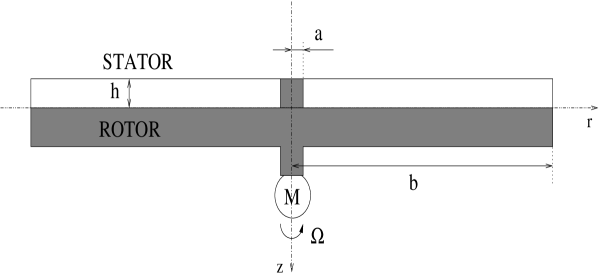
Figure 1: Randriamampianina et Poncet, Phys. Fluids.

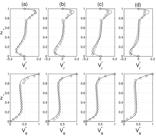
Figure 2: Randriamampianina et Poncet, Phys. Fluids.

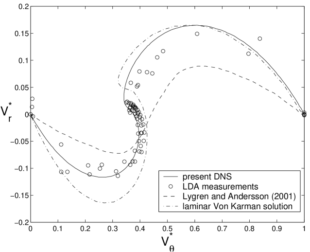
Figure 3: Randriamampianina et Poncet, Phys. Fluids.

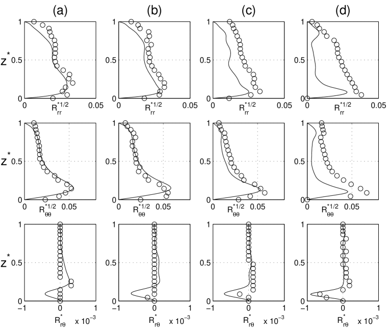
Figure 4: Randriamampianina et Poncet, Phys. Fluids.

Figure 5: Randriamampianina et Poncet, Phys. Fluids.

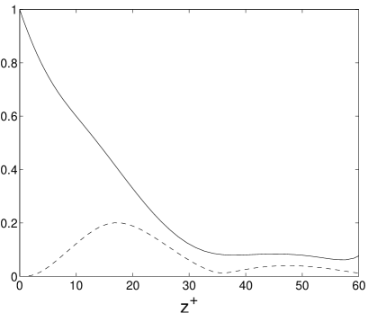
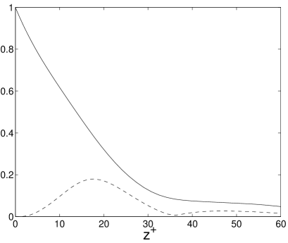
(a)	(b)

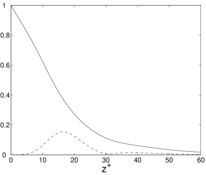
(c)

Figure 6: Randriamampianina et Poncet, Phys. Fluids.

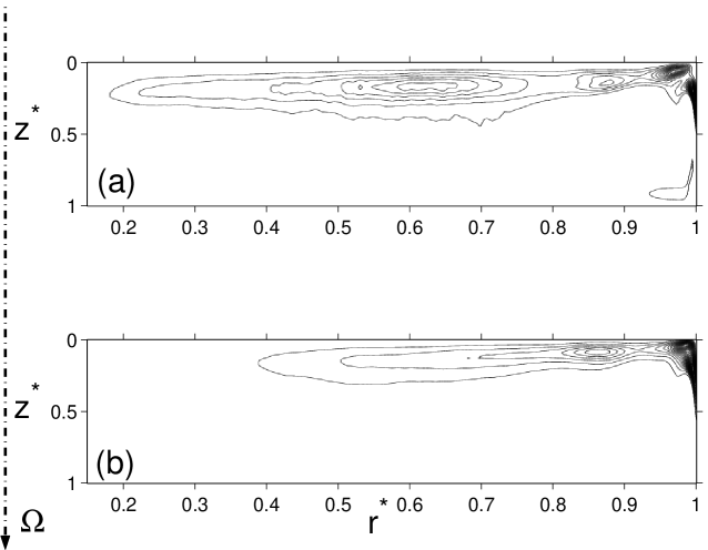
Figure 7: Randriamampianina et Poncet, Phys. Fluids.

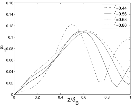
Figure 8: Randriamampianina et Poncet, Phys. Fluids.

Figure 9: Randriamampianina et Poncet, Phys. Fluids.

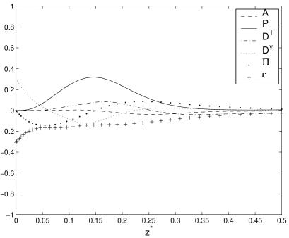
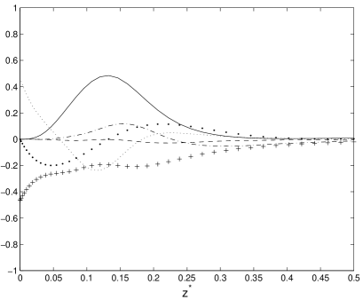
(a)	(b)

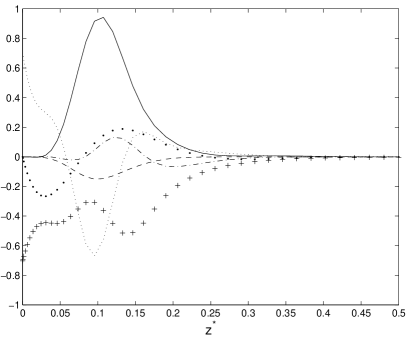
(c)

Figure 10: Randriamampianina et Poncet, Phys. Fluids.

Figure 11: Randriamampianina et Poncet, Phys. Fluids.

(a)	(b)

(c)

Figure 12: Randriamampianina et Poncet, Phys. Fluids.

$(a)$

$(b)$

Figure 13: Randriamampianina et Poncet, Phys. Fluids.

$(a)$

$(b)$

Figure 14: Randriamampianina et Poncet, Phys. Fluids.

$(a)$

$(b)$

Figure 15: Randriamampianina et Poncet, Phys. Fluids.

Appendix A Balance equations for the kinetic energy budgets in cylindrical coordinates

$$\overline{V_{j}}k_{,j}=-R_{ij}\overline{V_{i,j}}-\frac{1}{2}\overline{(v^{\prime}_{m}v^{\prime}_{j}v^{\prime}_{j})_{,m}}-\frac{1}{\rho}\overline{(v^{\prime}_{j}p^{\prime})_{,j}}-\nu\overline{v^{\prime}_{j,m}v^{\prime}_{j,m}}+\nu k_{,jj}$$ (6)

$$(a)\qquad\qquad(b)\qquad\qquad(c)\qquad\qquad(d)\qquad\qquad(e)\qquad\qquad(f)$$

Each instantaneous variable is decomposed in the following form:

$$f=\overline{f}+f^{\prime}$$

where $\overline{f}$ is the time averaged component and $f^{\prime}$ the fluctuating part. Using the normalizing scale $2\Omega^{3}h^{2}$ leads to the following dimensionless terms:

$$(a)\equiv G\overline{V}_{r}\partial_{r}k+\frac{G}{(r+R_{c})}\overline{V}_{\theta}\partial_{\theta}k+\overline{V}_{z}\partial_{z}k$$ (7)

$$(b)\equiv GR_{rr}\partial_{r}{\overline{V}_{r}}+R_{zz}\partial_{z}{\overline{V}_{z}}+GR_{rz}(\partial_{r}{\overline{V}_{z}}+\partial_{z}{\overline{V}_{r}})+$$

$$GR_{r\theta}(\partial_{r}\overline{V}_{\theta}+\frac{1}{(r+R_{c})}\partial_{\theta}\overline{V}_{r}-\frac{\overline{V}_{\theta}}{r+R_{c}})+$$

$$R_{z\theta}(\partial_{z}\overline{V}_{\theta}+\frac{\partial_{\theta}\overline{V}_{z}}{r+R_{c}})+GR_{\theta\theta}(\frac{\overline{V}_{r}}{r+R_{c}}+\frac{\partial_{\theta}\overline{V}_{\theta}}{r+R_{c}})$$ (8)

$$(c)\equiv G\partial_{r}\overline{(v^{\prime}_{r}k^{\prime})}+\partial_{z}\overline{(v^{\prime}_{z}k^{\prime})}+G\frac{\overline{v^{\prime}_{r}k^{\prime}}}{r+R_{c}}+\frac{G}{r+R_{c}}\partial_{\theta}\overline{(v^{\prime}_{\theta}k^{\prime})}$$ (9)

$$(d)\equiv G\partial_{r}\overline{(v^{\prime}_{r}p^{\prime})}+\partial_{z}\overline{(v^{\prime}_{z}p^{\prime})}+G\frac{\overline{v^{\prime}_{r}p^{\prime}}}{r+R_{c}}+\frac{G}{r+R_{c}}\partial_{\theta}\overline{(v^{\prime}_{\theta}p^{\prime})}$$ (10)

$$(e)\equiv\frac{R_{c}+1}{GRe}[G^{2}\overline{\partial_{r}v^{\prime}_{r}\partial_{r}v^{\prime}_{r}}+\overline{\partial_{z}v^{\prime}_{z}\partial_{z}v^{\prime}_{z}}+G^{2}\overline{\partial_{r}u^{\prime}_{z}\partial_{r}v^{\prime}_{z}}+\overline{\partial_{z}v^{\prime}_{r}\partial_{z}v^{\prime}_{r}}+$$

$$G^{2}\overline{\partial_{r}v^{\prime}_{\theta}\partial_{r}v^{\prime}_{\theta}}+\overline{\partial_{z}v^{\prime}_{\theta}\partial_{z}v^{\prime}_{\theta}}+G^{2}\overline{(\frac{1}{r+R_{c}}\partial_{\theta}v^{\prime}_{\theta}+\frac{v^{\prime}_{r}}{r+R_{c}})^{2}}+$$

$$G^{2}\overline{(\frac{1}{r+R_{c}}\partial_{\theta}v^{\prime}_{r}-\frac{v^{\prime}_{\theta}}{r+R_{c}})^{2}}+G^{2}\overline{\frac{\partial_{\theta}v^{\prime}_{\theta}\partial_{\theta}v^{\prime}_{\theta}}{(r+R_{c})^{2}}}]$$ (11)

$$(f)\equiv\frac{R_{c}+1}{GRe}(G^{2}\partial_{rr}k+\partial_{zz}k+G^{2}\frac{\partial_{r}k}{r+R_{c}}+\frac{G^{2}}{(r+R_{c})^{2}}\partial_{{\theta}{\theta}}k)$$ (12)

where

$$k^{\prime}=\frac{v^{\prime 2}_{r}+v^{\prime 2}_{\theta}+v^{\prime 2}_{z}}{2},\qquad k=\overline{\frac{v^{\prime 2}_{r}+v^{\prime 2}_{\theta}+v^{\prime 2}_{z}}{2}}=\overline{k^{\prime}},\qquad R_{ij}=\overline{v^{\prime}_{i}v^{\prime}_{j}}.$$