A New Approach To The Evaluation Of The $S$-Matrix In Atom-Diatom Quantum Reactive Scattering Theory

Ashot S. Gevorkyan gΛ™ashot@sci.am Institute for Informatics and Automation Problems, NAS of Armenia, P. Sevak St. 1, Yerevan 375014, Institute of Applied Problems in Physics, NAS Armenia, Nersisian St. 25, Yerevan 375014,    Gabriel G.Β Balint-Kurti Gabriel.Balint-Kurti@Bristol.ac.uk Center for Computational Chemistry, School of Chemistry, University of Bristol, Bristol BS8 1TS, UK    Gunnar Nyman nyman@chem.gu.se GΓΆteborg University, Department of Chemistry, SE-412 96, GΓΆteborg, Sweden
Abstract

A new approach is described to the evaluation of the S-matrix in three-dimensional atom-diatom reactive quantum scattering theory. The theory is developed based on natural collision coordinates where progress along the reaction coordinate can be viewed as fulfilling the same role as time in a time-dependent formulation. By writing the full wavefunction in coupled-channel form it is proved that the $3D$ quantum reactive scattering problem can be treated in the same way as an inelastic single-arrangement problem. In particularly, two types of coupled-channel representations, which are reduced to two different systems of coupled first order ordinary differential equations describing the inelastic scattering, are used. The first system of coupled differential equations is constructed on a set of points (grid) of the coordinate reaction curve after solution of many $1D$ SchrΓΆdinger problems in the directions normal to the reaction coordinate. The second expression for inelastic scattering is found using exactly solvable nonstationary $1D$ SchrΓΆdinger equation (etalon equation method), which is introduced for describing the localization properties of the full wavefunction along the curve of coordinate reaction. In this case we avoid a large amount of computation involved in solving the $1D$ SchrΓΆdinger problem along the reaction coordinate by using a slightly difficult initial conditions for the inelastic scattering equations. In both cases by solving the system of coupled first order ordinary differential equations, the full wavefunction and all S-matrix elements are obtained simultaneously without further calculations. Our analysis shows that the methods we have developed constitute the simplest algorithms for computing the reactive scattering S-matrices.

Quantum Scattering, Natural Collision Coordinate, Etalon Equation Method, S-matrix Elements, Coupled-Channel Differential Equations, Quantum Theory of Chemical Reactions

I Introduction

Accurate quantum dynamics approaches have made an immense impact on the theory of elementary atom-molecule collisions Schatz76 ; Kuppermann81 ; Manolopoulos . Recent advances in accurate quantum mechanical calculations on simple few atom systems have demonstrated the possibility of obtaining detailed information concerning chemical reactions from first principles Launay02 ; AJCP01 ; GBKSLLHYJCP00 . Tremendous progress has occurred in developing and applying both time-independent and time-dependent quantum dynamics approaches the last few years.

At present there are three common approaches used in the quantum reactive scattering field:

  1. 1.

    The hyperspherical coordinate methods Delves ; Schatz ,

  2. 2.

    The variational methods based on the simultaneous use of mass-scaled Jacobi coordinates in each of the chemical arrangements involved Miller ; BaerKouri ; MBaer and

  3. 3.

    Wavepacket methods Kosloff ; Kurti (many references can be found in the review Nyman ).

Both time-dependent and time-independent approaches have been successfully applied to three- and four-atom reactions. For detailed information at low energy the time-independent hyperspherical coordinate approach has proven the most useful Launay02 ; Manolopoulos2 . The time-dependent wavepacket method has also proved to be very useful, particularly for photodissociation and laser-molecule interaction problems. To go beyond four-atom systems, the Multi-Configurational Time-Dependent Hartree method has been applied in full-dimensionality to calculate thermal rate constants for the H + CH4 MZS and O + CH4 HNyman reactions.

Despite the successful applications to polyatomic systems mentioned above, general applications still appear to be extremely difficult. Quantum mechanics is nonlocal in character and numerical efforts to solve the SchrΓΆdinger equation increase exponentially with the number of degrees of freedom. State resolved accurate quantum dynamical calculations are presently limited to at most seven-dimensional problems MZS . Thus, the development of new conceptual approaches permitting improved computational algorithms for accurate quantum simulations is of great interest.

Earlier natural collision coordinates NCC allowing an analytical investigation of chemical reactivity in collinear collisions were introduced by Marcus Marcus and further explored by Light Light ; WLAJCP76 . Light and coworkers LightW ; SWL generalized the NCC approach to three-dimensional atom-diatom reactive scattering and on this basis they studied H + H2 system and its isotopomers in $3D$ for total angular momentum $J=0$ LightAl . Related developments have been the formulation and later use of the reaction-path hamiltonian formalism by Miller, Handy and Adams MHAJCP80 and the reaction path and reaction volume approaches advocated by Billing BMP96 ; KBJCP97 ; CBPCCP99 ; BCP02 .

Due to difficulties in applying the NCC approach, attention turned to other coordinate systems. Nevertheless, it seems to us that the primary idea of NCC, namely to simplify $3D$ quantum reactive scattering calculations, can be realized. Particularly, one of the authors has shown that for collinear three-body collisions, it is possible to constructed the S-matrix exactly, in simple form using the approach Ash ; Ash1 . Seven reactive systems, N2 + N, N2 + O, O2 + O, Li + FH, O2 + N etc have been studied successfully within this framework Ash2 .

The aim of the current article is to generalize our previous collinear NCC quantum scattering approach to a full three dimensional treatment.

II Quantum multi-channel scattering problem in different coordinate systems

The reactive scattering process in a three-body system can be described by the scheme:

$$A+(BC)_{n}\longrightarrow\begin{cases}A+(BC)_{m},\\ (AB)_{m}+C,\\ (AC)_{p}+B,\\ A+B+C,\\ \quad\quad\qquad(ABC)^{*}\longrightarrow\begin{cases}A+(BC)_{m},\\ (AB)_{m}+C,\\ (AC)_{p}+B,\\ A+B+C,\end{cases}\end{cases}$$
$$Sch.\,\,1.$$

where $A,B,$ and $C$ are atoms, $n$ and $m,p$ characterize quantum numbers of diatomic states corresponding to initial $(in)$ and final $(out)$ scattering channels, $(ABC)^{*}$ denotes an activated complex which may or may not be present as an intermediary species.

\arc705.1602.72554.6911\arc630.4021.53513.7494\blacken\ellipse254254\ellipse254254\blacken\ellipse254254\ellipse254254\blacken\ellipse254254\ellipse254254\blacken\ellipse254254\ellipse254254\blacken\ellipse254254\ellipse254254\blacken\ellipse254254\ellipse2542541620,4230)1620,945) 405,270)3600,2070) 6345,4185)8820,2970) 7110,3825)6570,720) A$\vec{R}_{\alpha}$ $\theta_{\alpha}$ $\vec{r}_{\alpha}$BCCAC$\vec{R}_{\beta}$ $\theta_{\beta}$ $\vec{r}_{\beta}$a)b)
Figure 1: Jacobi coordinates for the reaction $A+(BC)_{n}\rightarrow(AB)_{m}+C$ corresponding to the reactant (a) and to the product (b) channels.

II.1 The coordinate systems

We denote the masses of the particles by $m_{A},m_{B}$ and $m_{C}$ and the coordinates of the particles are denoted by the column vectors ${\bf{r_{A}}},{\bf{r_{B}}}$ and ${\bf{r_{C}}}$ describing their positions relative to an origin fixed in the laboratory system. The initial $9D$ problem can be reduced to a $6D$ one by elimination of the center-of-mass coordinates.

Below we consider the reaction $A+(BC)_{n}\rightarrow(ABC)^{\ast}\rightarrow(AB)_{m}+C$, i.e. there are two open arrangements.

For this reaction reactant and product Jacobi coordinates are illustrated in Fig.1. The following equations define the Jacobi coordinates $\bf{R}_{\alpha}$ and $\bf{r}_{\alpha}$ (note that index $\alpha$ corresponds to $(in)$ or reactant asymptotic channel):

$\displaystyle{\bf{R}}_{\alpha}={\bf{r}}_{A}-\frac{m_{B}{\bf{r_{B}}}+m_{C}{\bf{r_{C}}}}{m_{B}+m_{C}},\qquad{\bf{r}}_{\alpha}={\bf{r_{C}}}-{\bf{r_{B}}},\qquad\qquad$
$\displaystyle\Bigl{(}{\bf{R}}_{\alpha}\equiv{\bf{R}}_{\alpha}(R_{x},R_{y},R_{z}),\,\,\,{\bf{r}}_{\alpha}\equiv{\bf{r}}_{\alpha}(r_{x},r_{y},r_{z})\Bigr{)}.$ (1)

We now apply the Delves-Smith scale transformation Delves ; Smith ; MBaer to obtain the new scaled coordinates $\bf{q}_{0}$ and $\bf{q}_{1}$;

$\displaystyle{\bf{q}_{0}}\equiv{\bf{q}_{0\alpha}}=\lambda\,{\bf{R}}_{\alpha},\qquad{\bf{q}_{1}}\equiv{\bf{q}_{1\alpha}}=\lambda^{-1}\,{\bf{r}}_{\alpha}.\qquad$ (2)

where

$\displaystyle\lambda=\Bigl{[}\frac{m_{A}}{\mu}\Bigl{(}1-\frac{m_{A}}{M}\Bigr{)}\Bigr{]}^{1/2},\qquad\mu=\Bigl{[}\frac{m_{A}m_{B}m_{C}}{M}\Bigr{]}^{1/2},\qquad M=m_{A}+m_{B}+m_{C}.$ (3)

In these coordinates the Hamiltonian of a three-body system takes the following diagonal form:

$\displaystyle H\bigl{(}{\bf{q}};{\bf{P_{{\bf{q}}}}}\bigr{)}=\frac{1}{2\mu}{\bf{P}}_{\bf{q}}^{2}+V\bigl{(}q_{0},q_{1},\theta\bigr{)},\qquad\qquad\qquad$ (4)

where

$${\bf{q}}=\bigl{(}{\bf{q}_{0}},{\bf{q}_{1}})=\{q_{k}\},\quad k=0,...,5;\quad\{q_{k}\}=\bigl{(}q_{0}=|{\bf{q_{0}}}|,\,\,q_{1}=|{\bf{q_{1}}}|,\,\,q_{2},\,\,q_{3},\,\,q_{4},\,\,q_{5}\bigr{)}.$$

Note that here and in the following we omit the $\alpha$ channel index for simplicity. In Eq. (4) $\mu$ is the reduced mass defined in Eq. (3), ${\bf{P}_{\bf{q}}}$ is the moment vector conjugate to ${\bf{q}}$, in the body-fixed system and $\theta$ is the angle between vectors ${\bf{\bf{q_{0}}}}$ and ${\bf{q}_{1}}$ (see FIG. 1 and FIG. 2). An alternative coordinate system $(q_{0},q_{1},q_{2})$ is illustrated in FIG. 2. Either of the coordinate systems $(q_{0},q_{1},q_{2})$ and $(q_{0},q_{1},\theta)$ can be used to describe the motion of body-fixed system in the plane of the vectors $({\bf{q}_{0}},{\bf{q}_{1}})$ and they will be called intrinsic coordinates. The interaction potential between all atoms depends only on the intrinsic coordinates.

The coordinates $(q_{3},q_{4},q_{5})$ are taken to be the Euler angles $\Omega(\equiv\zeta_{1},\zeta_{2},\zeta_{3})$, which orient the three-body system in the space-fixed frame (see for example refs. Kurti , Edmonds and Zare ).

The optimal coordinate systems for reactants and products are different Miller ; PackPark . This fact creates certain mathematical and computational complexities in the investigation of the reactive scattering problem. One way to proceed is to turn to a special type of curvilinear coordinates which continuously leads from reactant channel to product channel. The possibility of introducing the coordinate system which is simultaneously suitable for description of $(in)$ and $(out)$ asymptotic states was first time discussed in the work Hof . At last corrected version for collinear collision was presented in the work Marcus and named natural collision coordinate (NCC) system.

In order to define the NCC appropriately, we connect the $(in)$ and $(out)$ asymptotic channels by a smooth curve $\Im_{if}$. The curve depends on two parameters, one of which can be chosen arbitrary and the other is system dependent. As progress along the curve represent the passage from reactant to product during this it will be called reaction coordinate Marcus ; Light .

\arc636.6712.97034.4301\blacken\ellipse284284\ellipse284284\arc636.6710.152.1\blacken\ellipse9090\ellipse9090\dottedline[.]100(1162,2497)(4425,2250) \blacken\ellipse202202\ellipse202202\blacken\ellipse284284\ellipse284284\blacken\ellipse9090\ellipse90902175,4590)1725,1080) 150,405)4425,2250) 150,405)2175,4635) AO$\theta^{\prime}$CBO$q_{1}$ $q_{0}$ $q_{2}$ $\theta$
Figure 2: The three-body system in mass-scaled Jacobi coordinates. The coordinate $q_{0}$ shows the distance between particle $A$ and the center of mass $(BC)$ pair $O$, the distance between particles $B$ and $C$ is $q_{1}$ and $q_{2}$ correspondingly between $A$ and $C$,   $\theta$ is a Jacobi scattering angle. The point $O^{\,{}^{\prime}}$ is a center of mass diatom $(AB)$ and $\theta^{\,{}^{\prime}}$ is correspondingly Jacobi scattering angle which is used in $(out)$ channel.

The curve $\Im_{if}$, which connects $(in)$ and $(out)$ asymptotic channels can be determined in the plane ($q_{0},q_{1},\theta=0$), by simple formula:

$$q_{0}^{c}=\frac{a}{q_{1}^{c}-q_{eq}^{-}}+b\bigl{(}q_{1}^{c}-q_{eq}^{-}\bigr{)}+q^{+}_{eq},\qquad q_{eq}^{-}<q_{1}^{c}<+\infty,$$ (5)

where $a$ and $b$ are constants.

Note that the collinear collision configuration $A+(BC)$ describes on the plane ($q_{0},q_{1},\theta=0$) while the collinear collision $A+(CB)$ describes on the plane ($q_{0},q_{1},\theta=\pi$). The motivation of choice of curve $\Im_{if}$ for later definition of $3D$ NCC system is given in the Appendix A. In Eq. (5) $q^{-}_{eq}$ and $q^{+}_{eq}$ are mass-scaled equilibrium bond lengths of molecules in the $(in)$ and $(out)$ channels correspondingly. Note that $a$ is an arbitrary constant, which is usually chosen to make the curve pass close to the saddle point of the reaction. The constant $b$ depends on the mass of particles and is given by expression $b=cot\varphi=\bigl{[}{m_{A}m_{C}}/{m_{B}M}\bigr{]}^{1/2}$. The superscript $c$ over $q_{0}$ and $q_{1}$ underlines the fact that the point $(q_{0}^{c},q_{1}^{c})$ lies on the curve.

The limit $q_{1}^{c}\rightarrow q_{eq}^{-},\,\,q_{0}^{c}\rightarrow{\infty}$ corresponds to the reactant region or $(in)$ channel while the limit $q_{1}^{c}\rightarrow\infty,\,\,q_{0}^{c}\rightarrow\infty$ on the curve $\Im_{if}$ corresponds to the product region or $(out)$ channel, where $q_{0}^{c}=bq_{1}^{c}+q^{+}_{eq}$. It is easy to show that the mass-scaled distance $q_{2}$ between $A$ and $B$ particles connected with the curve $\Im_{if}$ is described by expression $q_{2}^{c}=q_{2}\bigl{|}_{\Im_{if}}=\sqrt{(q_{0}^{c})^{2}-2bq_{0}^{c}q_{1}^{c}\cos\theta+b^{2}(q_{1}^{c})^{2}}$, which in the $(in)$ channel is equal $\bigl{(}q_{2}^{c}-q_{0}^{c}\bigr{)}\bigl{|}_{q_{1}^{c}\to q_{eq}^{-}}=-bq_{eq}^{-}\cos\theta$. In other words it is denote that in the $(in)$ channel curve $\Im_{if}$ is coming to the equilibrium distance $q_{eq}^{-}$ of $(BC)$ diatom. In the $(out)$ channel the curve $\Im_{if}$ approaches the equilibrium distance $q^{+}_{eq}$ of diatom $(AB)$ (see Appendix B). Note that the Jacobi scattering angle $\theta$ which defined in the reactant (or $(in)$) coordinates system in the product (or $(out)$) channel obviously must be limited to 00 inasmuch as the two sides $\overline{BO}=bq_{1}$ and $\overline{OA}=q_{0}$ of $\widehat{ABO}$ triangle are limited to infinity while the third side is limited to finite quantity $\overline{AB}=q_{2}\to q_{eq}^{+}$. Remaind that it doesn’t mean that the rotation of new-formed diatom $(AB)$ stops. The rotation of diatom $(AB)$ is described by angle $\theta^{\prime}$ (see FIG. 2) which in the reactant region is limited to 00 but beginning from strong interaction region up to $(out)$ asymptotic channel obviously can have any value.

The coordinate $u$ describes the translational motion of three-body system between reactant and product channels and is changed along the curve $\Im_{if}$ measured from an initial point $u_{0}$. It particularly can be determined by equation:

$$u=u_{0}-\frac{a}{q_{1}^{c}-q_{eq}^{-}}+b(q_{1}^{c}-q_{eq}^{-}\bigr{)}.$$ (6)

The signed distance from the curve $\Im_{if}$ in the plane ($q_{0},q_{1},\theta=0$) is given by $v$. We can organize the one-to-one mapping between coordinate systems $(q_{0},q_{1},\theta)$ and $(u,v,\theta)$ in only some subspace of internal 3D configuration space. It should be emphasized that above mentioned subspace must include a part of 3D space, in which the probability current of reactive scattering process is localized. This condition can be fulfilled if the coordinate reaction curve $\Im_{if}$ is correctly determined for a configuration of reactive collision with the minimal energy surface (see FIG. 3). It is obvious that in this case the condition of one-to-one mapping between coordinate systems for any configuration of reactive collision can be automatically satisfied.

After satisfying aforementioned condition it is easy to write transformations between set of coordinates $(q_{0},q_{1})$ and $(u,v)$ Light2 :

$\displaystyle q_{0}(u,v)=q_{0}^{c}(u)-v\sin\phi(u),$
$\displaystyle q_{1}(u,v)=q_{1}^{c}(u)+v\cos\phi(u),$ (7)

where the angle $\phi(u)$ is determined from the requirement that the coordinate system $(u,v)$ should be orthogonal (see Appendix C):

\arc414.8805.57466.5019\blacken\ellipse9090\ellipse9090\blacken\ellipse9090\ellipse9090\blacken\ellipse9090\ellipse9090\blacken\ellipse9090\ellipse9090\blacken\ellipse9090\ellipse9090\blacken\ellipse9090\ellipse9090\blacken\ellipse9090\ellipse9090\blacken\ellipse9090\ellipse9090\blacken\ellipse9090\ellipse90904279,308)4279,2344) 4301.620,2253.520)4279.000,2344.000)(4256.380,2253.520) 4279,308)6314,308)(6348,308) 6257.520,285.380)6348.000,308.000)(6257.520,330.620) 4279,308)6111,1054) 6035.732,998.927)6111.000,1054.000)(6018.670,1040.826) \drawline(4275,274)(4275,274) 4365,2299)4365,2297)(4365,2294) (4366,2288)(4367,2279)(4367,2268) (4369,2253)(4370,2236)(4372,2217) (4374,2197)(4377,2174)(4379,2150) (4383,2123)(4387,2094)(4391,2061) (4397,2024)(4403,1983)(4410,1939) (4417,1899)(4423,1860)(4429,1826) (4434,1797)(4438,1773)(4441,1754) (4444,1740)(4445,1728)(4446,1719) (4448,1710)(4449,1702)(4450,1693) (4452,1681)(4455,1667)(4459,1648) (4464,1625)(4471,1597)(4479,1564) (4489,1527)(4500,1489)(4513,1448) (4524,1411)(4535,1381)(4543,1357) (4550,1340)(4555,1327)(4558,1319) (4561,1313)(4564,1309)(4566,1305) (4569,1300)(4573,1293)(4579,1283) (4586,1269)(4595,1251)(4607,1228) (4620,1202)(4635,1174)(4654,1141) (4669,1114)(4681,1093)(4688,1080) (4691,1072)(4692,1068)(4691,1065) (4691,1063)(4693,1060)(4697,1054) (4706,1045)(4722,1031)(4743,1013) (4770,994)(4796,978)(4820,965) (4841,954)(4857,946)(4869,941) (4878,938)(4885,935)(4890,934) (4896,933)(4903,931)(4913,929) (4927,926)(4947,922)(4973,916) (5004,910)(5040,904)(5076,899) (5109,896)(5136,893)(5157,892) (5173,892)(5184,892)(5191,892) (5198,893)(5204,894)(5211,895) (5222,896)(5238,897)(5259,898) (5286,900)(5319,902)(5355,904) (5390,907)(5421,910)(5445,912) (5462,914)(5473,915)(5479,915) (5482,915)(5483,915)(5486,916) (5493,917)(5505,920)(5524,924) (5550,930)(5585,939)(5625,949) (5659,958)(5693,968)(5725,978) (5756,987)(5786,997)(5814,1006) (5841,1015)(5867,1024)(5892,1033) (5916,1042)(5939,1050)(5960,1058) (5979,1065)(5995,1071)(6008,1076) (6018,1079)(6025,1082)(6028,1083)(6030,1084) \texture55888888 88555555 5522a222 a2555555 55888888 88555555 552a2a2a 2a555555 55888888 88555555 55a222a2 22555555 55888888 88555555 552a2a2a 2a555555 55888888 88555555 5522a222 a2555555 55888888 88555555 552a2a2a 2a555555 55888888 88555555 55a222a2 22555555 55888888 88555555 552a2a2a 2a555555 \shade4950,1804)4950,1803)(4950,1800) (4950,1790)(4950,1774)(4949,1752) (4949,1726)(4948,1697)(4947,1668) (4947,1640)(4945,1614)(4944,1590) (4943,1569)(4941,1549)(4940,1531) (4937,1513)(4935,1496)(4932,1477) (4928,1458)(4924,1439)(4920,1419) (4915,1399)(4909,1379)(4904,1359) (4898,1340)(4893,1322)(4887,1305) (4882,1289)(4877,1275)(4872,1261) (4868,1249)(4860,1229)(4853,1212) (4847,1196)(4843,1182)(4840,1172) (4839,1164)(4841,1160)(4845,1159) (4850,1160)(4857,1162)(4865,1166) (4876,1171)(4888,1178)(4901,1186) (4915,1194)(4929,1202)(4943,1211) (4958,1219)(4970,1226)(4983,1233) (4996,1240)(5011,1248)(5026,1256) (5041,1264)(5057,1272)(5072,1280) (5087,1288)(5102,1295)(5116,1302) (5130,1309)(5142,1315)(5154,1321) (5166,1327)(5179,1334)(5193,1341) (5207,1348)(5221,1355)(5235,1362) (5250,1370)(5264,1377)(5278,1385) (5291,1392)(5304,1399)(5318,1406) (5331,1414)(5345,1422)(5360,1431) (5376,1440)(5395,1451)(5416,1463) (5438,1476)(5462,1490)(5485,1504) (5505,1516)(5521,1526)(5530,1531) (5534,1534)(5535,1534) 4950,1804)4950,1803)(4950,1800) (4950,1790)(4950,1774)(4949,1752) (4949,1726)(4948,1697)(4947,1668) (4947,1640)(4945,1614)(4944,1590) (4943,1569)(4941,1549)(4940,1531) (4937,1513)(4935,1496)(4932,1477) (4928,1458)(4924,1439)(4920,1419) (4915,1399)(4909,1379)(4904,1359) (4898,1340)(4893,1322)(4887,1305) (4882,1289)(4877,1275)(4872,1261) (4868,1249)(4860,1229)(4853,1212) (4847,1196)(4843,1182)(4840,1172) (4839,1164)(4841,1160)(4845,1159) (4850,1160)(4857,1162)(4865,1166) (4876,1171)(4888,1178)(4901,1186) (4915,1194)(4929,1202)(4943,1211) (4958,1219)(4970,1226)(4983,1233) (4996,1240)(5011,1248)(5026,1256) (5041,1264)(5057,1272)(5072,1280) (5087,1288)(5102,1295)(5116,1302) (5130,1309)(5142,1315)(5154,1321) (5166,1327)(5179,1334)(5193,1341) (5207,1348)(5221,1355)(5235,1362) (5250,1370)(5264,1377)(5278,1385) (5291,1392)(5304,1399)(5318,1406) (5331,1414)(5345,1422)(5360,1431) (5376,1440)(5395,1451)(5416,1463) (5438,1476)(5462,1490)(5485,1504) (5505,1516)(5521,1526)(5530,1531) (5534,1534)(5535,1534) (4365,2254)(4367,2251)(4370,2246) (4376,2236)(4385,2221)(4397,2202) (4463,2093)(4481,2063)(4499,2035) (4516,2008)(4531,1982)(4546,1959) (4560,1937)(4572,1917)(4584,1899) (4596,1881)(4607,1865)(4617,1849) (4628,1834)(4640,1816)(4653,1798) (4666,1780)(4679,1763)(4692,1745) (4706,1727)(4720,1710)(4735,1692) (4750,1675)(4764,1659)(4779,1643) (4794,1627)(4809,1612)(4824,1599) (4839,1585)(4853,1573)(4868,1561) (4925,1518)(4940,1508)(4956,1498) (4973,1488)(4990,1477)(5008,1467) (5027,1456)(5046,1446)(5066,1436) (5086,1426)(5105,1416)(5125,1406) (5145,1397)(5165,1388)(5184,1379) (5204,1371)(5223,1362)(5243,1354) (5262,1346)(5283,1337)(5303,1329) (5325,1320)(5347,1312)(5370,1303) (5394,1293)(5418,1284)(5442,1275) (5466,1266)(5491,1257)(5515,1248) (5539,1240)(5562,1231)(5584,1224) (5606,1216)(5627,1209)(5647,1202) (5666,1195)(5685,1189)(5705,1182) (5726,1176)(5746,1169)(5766,1163) (5788,1156)(5811,1149)(5835,1142) (5861,1134)(5888,1126)(5915,1118) \shade5445,2704)5445,2703)(5445,2700) (5445,2690)(5445,2674)(5444,2652) (5444,2625)(5443,2596)(5442,2567) (5442,2538)(5440,2512)(5439,2487) (5438,2465)(5436,2445)(5435,2426) (5432,2407)(5430,2389)(5427,2371) (5424,2353)(5421,2334)(5417,2315) (5413,2296)(5409,2277)(5404,2258) (5400,2239)(5396,2221)(5391,2203) (5387,2187)(5383,2173)(5379,2159) (5376,2147)(5373,2136)(5370,2126) (5369,2123)(5368,2120)(5367,2117) (5366,2114)(5366,2111)(5365,2109) (5364,2106)(5364,2104)(5363,2101) (5362,2099)(5362,2097)(5361,2095) (5361,2094)(5360,2092)(5360,2091) (5360,2090)(5360,2088)(5359,2087) (5359,2086)(5359,2085)(5360,2085) (5360,2086)(5361,2086)(5361,2087) (5362,2088)(5362,2089)(5363,2090) (5364,2091)(5364,2092)(5365,2094) (5366,2095)(5366,2097)(5367,2099) (5368,2100)(5369,2102)(5370,2104) (5374,2111)(5378,2120)(5384,2130) (5390,2141)(5397,2154)(5405,2167) (5414,2181)(5424,2195)(5434,2208) (5445,2222)(5456,2234)(5468,2246) (5478,2257)(5490,2267)(5502,2277) (5516,2288)(5530,2298)(5546,2309) (5562,2319)(5578,2330)(5595,2340) (5612,2349)(5629,2358)(5645,2366) (5661,2374)(5678,2381)(5692,2388) (5707,2394)(5722,2401)(5739,2407) (5757,2414)(5777,2422)(5800,2430) (5824,2438)(5849,2447)(5873,2456) (5896,2464)(5915,2470)(5928,2475) (5936,2478)(5939,2479)(5940,2479) 5445,2704)5445,2703)(5445,2700) (5445,2690)(5445,2674)(5444,2652) (5444,2625)(5443,2596)(5442,2567) (5442,2538)(5440,2512)(5439,2487) (5438,2465)(5436,2445)(5435,2426) (5432,2407)(5430,2389)(5427,2371) (5424,2353)(5421,2334)(5417,2315) (5413,2296)(5409,2277)(5404,2258) (5400,2239)(5396,2221)(5391,2203) (5387,2187)(5383,2173)(5379,2159) (5376,2147)(5373,2136)(5370,2126) (5369,2123)(5368,2120)(5367,2117) (5366,2114)(5366,2111)(5365,2109) (5364,2106)(5364,2104)(5363,2101) (5362,2099)(5362,2097)(5361,2095) (5361,2094)(5360,2092)(5360,2091) (5360,2090)(5360,2088)(5359,2087) (5359,2086)(5359,2085)(5360,2085) (5360,2086)(5361,2086)(5361,2087) (5362,2088)(5362,2089)(5363,2090) (5364,2091)(5364,2092)(5365,2094) (5366,2095)(5366,2097)(5367,2099) (5368,2100)(5369,2102)(5370,2104) (5374,2111)(5378,2120)(5384,2130) (5390,2141)(5397,2154)(5405,2167) (5414,2181)(5424,2195)(5434,2208) (5445,2222)(5456,2234)(5468,2246) (5478,2257)(5490,2267)(5502,2277) (5516,2288)(5530,2298)(5546,2309) (5562,2319)(5578,2330)(5595,2340) (5612,2349)(5629,2358)(5645,2366) (5661,2374)(5678,2381)(5692,2388) (5707,2394)(5722,2401)(5739,2407) (5757,2414)(5777,2422)(5800,2430) (5824,2438)(5849,2447)(5873,2456) (5896,2464)(5915,2470)(5928,2475) (5936,2478)(5939,2479)(5940,2479) $\varphi$b)\arc414.8805.57466.5019904,308)904,2344) 926.620,2253.520)904.000,2344.000)(881.380,2253.520) 904,308)2939,308)(2973,308) 2882.520,285.380)2973.000,308.000)(2882.520,330.620) 904,308)2736,1054) 2660.732,998.927)2736.000,1054.000)(2643.670,1040.826) \drawline(900,274)(900,274) 1215,1039)1575,769) 1461.000,817.000)1575.000,769.000)(1497.000,865.000) 1215,1039)1485,1309) 1421.360,1202.934)1485.000,1309.000)(1378.934,1245.360) 1215,1039)1170,1309) 1219.320,1195.565)1170.000,1309.000)(1160.136,1185.701) 900,319)675,1084) 737.641,977.341)675.000,1084.000)(680.079,960.411) 855,454)855,724)(900,544) 1005,2276)1005,2273)(1006,2266) (1006,2253)(1008,2234)(1009,2209) (1011,2178)(1013,2143)(1016,2106) (1018,2068)(1021,2029)(1023,1992) (1026,1957)(1028,1924)(1030,1894) (1032,1865)(1034,1839)(1037,1814) (1039,1791)(1041,1769)(1043,1748) (1045,1727)(1047,1705)(1050,1683) (1052,1660)(1055,1638)(1058,1616) (1061,1593)(1064,1571)(1067,1548) (1070,1526)(1074,1504)(1077,1483) (1081,1462)(1084,1442)(1088,1423) (1091,1404)(1094,1387)(1098,1371) (1101,1355)(1104,1340)(1107,1326) (1111,1306)(1116,1287)(1121,1268) (1126,1250)(1131,1232)(1137,1214) (1143,1196)(1149,1180)(1155,1164) (1161,1149)(1167,1135)(1173,1123) (1180,1111)(1186,1099)(1194,1087) (1203,1074)(1213,1061)(1223,1049) (1235,1036)(1247,1024)(1260,1012) (1273,1001)(1287,990)(1300,981) (1314,972)(1328,964)(1340,958) (1354,951)(1368,945)(1383,939) (1399,933)(1415,928)(1433,923) (1450,918)(1468,914)(1486,911) (1503,908)(1520,905)(1537,903) (1554,902)(1569,901)(1584,901) (1599,901)(1615,901)(1632,901) (1650,902)(1668,904)(1686,905) (1705,907)(1724,909)(1742,911) (1761,914)(1779,916)(1796,919) (1814,922)(1831,925)(1849,928) (1867,931)(1886,934)(1905,938) (1926,941)(1947,945)(1968,950) (1989,954)(2011,958)(2032,962) (2053,967)(2074,971)(2093,975) (2112,979)(2130,983)(2148,987) (2165,991)(2183,995)(2200,999) (2218,1003)(2236,1007)(2255,1012) (2273,1016)(2291,1020)(2309,1025) (2327,1029)(2344,1034)(2360,1038) (2376,1042)(2391,1046)(2405,1050) (2419,1054)(2434,1059)(2450,1063) (2466,1068)(2483,1073)(2501,1079) (2521,1085)(2543,1092)(2566,1100) (2587,1107)(2606,1113)(2621,1118) (2630,1121)(2633,1122)(2634,1122) \dashline60.000(450,2884)(450,2881)(451,2873) (452,2861)(454,2842)(457,2818) (460,2789)(464,2758)(467,2725) (471,2693)(475,2662)(478,2632) (481,2605)(485,2580)(488,2557) (491,2536)(494,2516)(496,2498) (499,2481)(503,2464)(506,2444) (511,2424)(515,2404)(520,2384) (525,2364)(530,2345)(535,2326) (541,2307)(547,2290)(552,2273) (558,2257)(564,2242)(569,2229) (575,2216)(580,2205)(585,2194) (592,2181)(599,2168)(607,2156) (615,2145)(624,2134)(634,2123) (645,2113)(656,2104)(667,2096) (679,2088)(692,2081)(705,2074) (717,2068)(730,2062)(745,2056) (760,2050)(777,2044)(794,2039) (812,2033)(830,2028)(848,2024) (866,2020)(883,2018)(899,2016) (915,2014)(930,2014)(945,2014) (959,2016)(974,2018)(988,2021) (1003,2025)(1017,2030)(1032,2035) (1046,2042)(1060,2049)(1072,2056) (1085,2064)(1096,2072)(1107,2080) (1118,2089)(1128,2098)(1138,2108) (1148,2118)(1159,2130)(1169,2142) (1179,2155)(1189,2168)(1199,2182) (1208,2197)(1217,2211)(1225,2226) (1232,2240)(1239,2254)(1245,2269) (1250,2282)(1255,2296)(1259,2310) (1264,2325)(1268,2341)(1272,2358) (1276,2375)(1279,2393)(1283,2411) (1286,2430)(1288,2448)(1291,2467) (1293,2485)(1295,2503)(1296,2521) (1298,2539)(1299,2555)(1300,2572) (1300,2589)(1301,2608)(1302,2629) (1302,2651)(1303,2675)(1303,2702) (1304,2730)(1304,2759)(1304,2788) (1305,2816)(1305,2840)(1305,2859) (1305,2873)(1305,2880)(1305,2884) \dashline60.000(2835,1669)(2832,1667)(2826,1663) (2816,1656)(2802,1646)(2784,1634) (2763,1619)(2741,1604)(2719,1588) (2697,1573)(2677,1558)(2659,1544) (2642,1532)(2626,1519)(2612,1508) (2598,1497)(2585,1485)(2573,1474) (2558,1461)(2544,1447)(2530,1433) (2515,1418)(2501,1403)(2486,1386) (2472,1370)(2458,1353)(2444,1336) (2431,1319)(2419,1302)(2407,1286) (2397,1271)(2387,1255)(2378,1241) (2370,1226)(2362,1210)(2354,1194) (2347,1177)(2340,1161)(2334,1143) (2328,1126)(2324,1109)(2320,1091) (2317,1075)(2314,1059)(2312,1043) (2311,1029)(2310,1015)(2310,1001) (2310,986)(2311,971)(2313,955) (2316,939)(2319,923)(2324,907) (2329,892)(2336,877)(2343,864) (2351,851)(2360,840)(2370,829) (2379,820)(2390,812)(2401,804) (2414,796)(2428,788)(2444,781) (2461,774)(2479,768)(2497,763) (2516,758)(2535,754)(2555,751) (2575,748)(2595,746)(2611,746) (2628,745)(2646,745)(2665,745) (2684,745)(2705,746)(2726,748) (2748,750)(2770,752)(2792,754) (2814,757)(2836,760)(2857,764) (2878,767)(2898,771)(2918,775) (2937,780)(2955,784)(2973,789) (2991,794)(3010,799)(3029,805) (3049,812)(3071,820)(3094,828) (3119,838)(3145,848)(3172,858) (3199,869)(3224,879)(3245,888) (3263,895)(3275,900)(3282,903)(3285,904) a)$(in)$ $(out)$ $\Im_{ij}$ ${q}_{1}$ $\varphi$ $q_{2}$ $v$ $u$ $q_{0}$ $q_{0}$ ${q}_{1}^{c}$
Figure 3: a) Intrinsic 3D Jacobi and natural collision coordinate (NCC) systems. The angle $\varphi$ is defined in the text. b) The reaction path (cycled curve) is passing through the minimums of potential energy while the reaction coordinate $\Im_{if}$ can be an arbitrary smooth curve connecting $(in)$ and $(out)$ asymptotic channels. The lower shaded area is self-crossing region for NCC system associated to the reaction path curve while the upper one self-crossing region for NCC system is associated to the curve $\Im_{if}$.
$$\frac{dq_{0}^{c}}{dq_{1}^{c}}\biggl{|}_{(u,v=0)}=\cot\phi(u),\qquad\lim_{u\rightarrow+\infty}\cot\phi(u)=\cot\varphi.$$ (8)

In the NCC system the motions of the body system are locally factorized into translational $\bigl{(}u$, infinite extension$\bigr{)}$, vibrational $\bigl{(}v$, finite$\bigr{)}$ and intrinsic rotational ($\theta$, finite) motions. Note that the coordinate $u$ is perpendicular to the curve $v$ and independent from the angle $\theta$. These properties ensure that the full wavefunction can be conditionally (locally) factorized.

So, we defined NCC system for investigation of $3D$ reactive quantum scattering which for using has only one limitation related with the region of self-crossing of coordinate lines. In other words it is necessary to choose the reaction coordinate $\Im_{if}$ in such a way in order to the probability current of quantum reactive scattering process in the region of self-crossing of coordinate line was absent.

III Quantum reactive scattering in the NCC system

III.1 Equation of motion of the three-body system

The overall stationary wavefunction of three-body system can be written as:

$$\Psi^{JM}(q_{0},q_{1},\theta,\Omega)=\frac{1}{q_{0}q_{1}}\sum_{K}\overline{\Phi}^{J}_{K}(q_{0},q_{1},\theta)D^{J}_{KM}(\Omega),$$ (9)

where $J$ is the total angular momentum, $M$ and $K$ are its space-fixed and body-fixed $z$-components respectively. The summation over $K$ ranges from $-J$ to $+J$ in unit steps and $D^{J}_{KM}$ is the Wigner $D$-matrix Edmonds ; Zare .

After separation of the external rotations, the action of the hamiltonian on the wavefunction is given by the formula Kurti ; WLAJCP76 :

$\displaystyle\hat{H}\overline{\Phi}^{J}_{K}(q_{0},q_{1},\theta)$ $\displaystyle=$ $\displaystyle-\frac{\hbar^{2}}{2\mu}\biggl{\{}\frac{\partial^{2}}{\partial{q_{0}^{2}}}+\frac{\partial^{2}}{\partial{q_{1}^{2}}}\biggr{\}}\,\overline{\Phi}^{J}_{K}(q_{0},q_{1},\theta)\qquad\qquad\qquad\qquad\qquad\qquad\,\,\qquad$ (10)
$\displaystyle-\,\frac{\hbar^{2}}{2\mu}\biggl{(}\frac{q_{0}^{2}+q_{1}^{2}}{q_{0}^{2}q^{2}_{1}}\biggr{)}\biggl{\{}\frac{1}{\sin\theta}\frac{\partial}{\partial{\theta}}\sin\theta\frac{\partial}{\partial{\theta}}-\frac{K^{2}}{\sin^{2}\theta}\biggr{\}}\,\overline{\Phi}^{J}_{K}(q_{0},q_{1},\theta)\qquad\quad\,\,\,\,$
$\displaystyle+\,V(R,r,\theta)\overline{\Phi}^{J}_{K}(q_{0},q_{1},\theta)+\frac{\hbar^{2}}{2\mu{q_{0}^{2}}}\Bigl{(}J(J+1)-2K^{2}\Bigr{)}\,\overline{\Phi}^{J}_{K}(q_{0},q_{1},\theta)\qquad$
$\displaystyle-\,\frac{\hbar^{2}}{2\mu{q_{0}^{2}}}\,c^{+}_{JK}\biggl{\{}\frac{\partial}{\partial{\theta}}-(K+1)\cot\theta\biggr{\}}\,\overline{\Phi}^{J}_{(K+1)}(q_{0},q_{1},\theta)$
$\displaystyle+\,\frac{\hbar^{2}}{2\mu{q_{0}^{2}}}\,c^{-}_{JK}\biggl{\{}\frac{\partial}{\partial{\theta}}+(K-1)\cot\theta\biggr{\}}\,\overline{\Phi}^{J}_{(K-1)}(q_{0},q_{1},\theta)$
$\displaystyle=$ $\displaystyle E\,\overline{\Phi}^{J}_{K}(q_{0},q_{1},\theta),$

where

$$c^{\pm}_{JK}=\bigl{[}J(J+1)-K(K\pm 1)\bigr{]}^{1/2}.$$ (11)

After the coordinate transformation $(q_{0},q_{1},\theta)\rightarrow(u,v,\theta)$ in equation (10) we find:

$\displaystyle\hat{H}\overline{\Phi}^{J}_{K}(u,v,\theta)$ $\displaystyle=$ $\displaystyle-\frac{\hbar^{2}}{2\mu}\frac{1}{\eta}\biggl{\{}\frac{\partial}{\partial{u}}\frac{1}{\eta}\frac{\partial}{\partial{u}}+\frac{\partial}{\partial{v}}\eta\,\frac{\partial}{\partial{v}}\biggr{\}}\overline{\Phi}^{J}_{K}(u,v,\theta)-\frac{\,\hbar^{2}}{2\mu}\frac{1}{\,q^{2}(u,v)}\times$ (12)
$\displaystyle\times\biggl{\{}\frac{1}{\sin\theta}\frac{\partial}{\partial{\theta}}\sin\theta\frac{\partial}{\partial{\theta}}-\frac{K^{2}}{\sin^{2}\theta}\biggr{\}}\overline{\Phi}^{J}_{K}(u,v,\theta)+U(u,v,\theta)\overline{\Phi}^{J}_{K}(u,v,\theta)$
$\displaystyle+E_{JK}\overline{\Phi}^{J}_{K}(u,v,\theta)+\frac{\hbar^{2}}{2\mu}\biggl{\{}H^{+}_{JK}\overline{\Phi}^{J}_{(K+1)}(u,v,\theta)+H^{-}_{JK}\overline{\Phi}^{J}_{(K-1)}(u,v,\theta)\biggr{\}}$
$\displaystyle=$ $\displaystyle E\,\overline{\Phi}^{J}_{K}(u,v,\theta),$

where

$$E_{JK}(u,v)=\frac{\hbar^{2}}{2\mu q_{0}^{2}(u,v)}\Bigl{(}J(J+1)-2K^{2}\Bigr{)},\quad H^{\pm}_{JK}=\frac{c^{\pm}_{JK}}{q_{0}^{2}(u,v)}\,\biggl{\{}\mp\frac{\partial}{\partial{\theta}}+\,(K\pm\,1)\cot\theta\biggr{\}},$$
$\displaystyle q^{2}(u,v)=\frac{q_{0}^{2}(u,v)q_{1}^{2}(u,v)}{q_{0}^{2}(u,v)+q_{1}^{2}(u,v)},\quad V(R,r,\theta)\equiv\,U(u,v,\theta),\quad\overline{\Phi}^{J}_{K}(q_{0},q_{1},\theta)\equiv\overline{\Phi}^{J}_{K}(u,v,\theta).\quad$ (13)

In expression (12) the LamΓ© coefficient $\eta(u,v)$ has a form (Appendix C):

$$\eta(u,v)=\bigl{[}1+K(u)v\bigr{]}\frac{ds}{du},$$ (14)

where $K(u)$ is described curvature of the reaction coordinate $\Im_{ij}$ in the continues point $u$, correspondingly $s$ the length along the $\Im_{ij}$:

$$K(u)=\frac{2a}{\bigl{(}q_{1}^{c}-q_{eq}^{-}\bigr{)}^{3}}\biggl{\{}1+\Bigl{[}b-a/{\bigl{(}q_{1}^{c}-q_{eq}^{-}\bigr{)}^{2}}\Bigr{]}^{2}\biggr{\}}^{-3/2},$$ (15)

and

$$\frac{ds}{du}=\biggl{\{}1+\Bigl{[}b-a/{\bigl{(}q_{1}^{c}-q_{eq}^{-}\bigr{)}^{2}}\Bigr{]}^{2}\biggr{\}}^{1/2}\biggl{\{}b+a/{\bigl{(}q_{1}^{c}-q_{eq}^{-}\bigr{)}^{2}}\biggr{\}}^{-1}.$$ (16)

Finally we transform Eq. (12) by setting $\overline{\Phi}^{J}_{K}(u,v,\theta)=\eta^{-1/2}{\Phi}^{J}_{K}(u,v,\theta)$, whereby we obtain:

$\displaystyle\biggl{\{}\biggl{[}\frac{\partial}{\partial{u}}\frac{1}{\eta^{2}}\frac{\partial}{\partial{u}}+\frac{\partial^{2}}{\partial{v^{2}}}\biggr{]}+\frac{1}{q^{2}(u,v)}\biggl{[}\frac{1}{\sin\theta}\frac{\partial}{\partial{\theta}}\sin\theta\frac{\partial}{\partial{\theta}}-\frac{K^{2}}{\sin^{2}\theta}\biggr{]}+\frac{2\mu}{\hbar^{2}}\bigl{[}E-U(u,v,\theta)-\qquad$
$\displaystyle E_{JK}(u,v)-U_{eff}(u,v)\bigr{]}\biggr{\}}{\Phi}^{J}_{K}(u,v,\theta)+\biggl{\{}H^{+}_{JK}{\Phi}^{J}_{(K+1)}(u,v,\theta)+H^{-}_{JK}{\Phi}^{J}_{(K-1)}(u,v,\theta)\biggr{\}}=0,$
(17)

where the effective potential $U_{eff}(u,v)$ is defined by

$\displaystyle U_{eff}(u,v)=\frac{1}{4\eta^{2}}\biggl{(}\frac{\partial\eta}{\partial{v}}\biggr{)}^{2}-\frac{1}{2\eta^{3}}\frac{\partial^{2}\eta}{\partial{u^{2}}}+\frac{5}{4\eta^{4}}\biggl{(}\frac{\partial\eta}{\partial{u}}\biggr{)}^{2}.$ (18)

SchrΓΆdinger equation (17) is in a form which is suitable for further investigation by the coupled channels method. This will be done in section III. C after the S-matrix has been defined in Section III. B.

III.2 Definition of S-matrix in term of reaction coordinate

In the standard scattering theory the main problem is the construction of the scattering S-matrix, holding the transition amplitudes. Let us discuss the exact representation for the S-matrix in terms of overlap between stationary wavefunctions (see for example New ; GoldWat ). In the body-fixed NCC system we can write the following general formal expression:

$$\Phi^{(+)J}_{njK}(u_{\alpha},v_{\alpha},\theta_{\alpha})=\sum_{n^{\prime}j\,^{\prime}K^{\prime}}\emph{S}^{J}_{n^{\prime}j\,^{\prime}K^{\prime}\,\leftarrow\,nj\,K}\,\Phi^{(-)J}_{n^{\prime}j\,^{\prime}K^{\prime}}(u_{\beta},v_{\beta},\theta_{\beta}),$$ (19)

where $\Phi^{(+)J}_{njK}(u_{\alpha},v_{\alpha},\theta_{\alpha})$ and $\Phi^{(-)J}_{n^{\prime}j\,^{\prime}K^{\prime}}(u_{\beta},v_{\beta},\theta_{\beta})$ are the total stationary wavefunctions in correspondingly NCC systems which are evaluating from some clear $(in)$ and $(out)$ asymptotic states, $n$ and $j$ are vibration and rotation quantum numbers, $\emph{S}_{n^{\prime}j\,^{\prime}K^{\prime}\,\leftarrow\,njK}^{J}$ are an complex matrix elements.

For the overall wavefunction ${\Phi}^{(+)J}_{njK}(u,v,\theta)$ we may enforce the following asymptotic behaviors and boundary conditions:

$\displaystyle{\Phi}^{(+)J}_{njK}(u,v,\theta)\,\,\stackrel{{\scriptstyle\sim}}{{{}_{u\rightarrow-\infty}}}\,\,{\Phi}_{njK}^{(in)J}(u,v,\theta),\qquad\qquad\qquad\qquad\qquad$
$\displaystyle{\Phi}^{(+)J}_{njK}(u,v,\theta)\,\,\stackrel{{\scriptstyle\sim}}{{{}_{u\rightarrow+\infty}}}\,\,\sum_{n^{\prime}j\,^{\prime}K^{\prime}}S^{J}_{njK\,\leftarrow\,n^{\prime}j\,^{\prime}K^{\prime}}\,(E)\,{\Phi}_{n^{\prime}j\,^{\prime}K^{\prime}}^{(out)J}(u,v,\theta),$
$\displaystyle\lim_{|v|\rightarrow\infty}{\Phi}^{(+)J}_{njK}(u,v,\theta)=\lim_{|v|\rightarrow\infty}\frac{\partial}{\partial{v}}{\Phi}^{(+)J}_{njK}(u,v,\theta)=0.\qquad\qquad\quad\quad$ (20)

where ${\Phi}_{njK}^{(in)J}(u,v,\theta)$ and ${\Phi}_{n^{\prime}j\,^{\prime}K^{\prime}}^{(out)J}(u_{\beta},v_{\beta},\theta_{\beta})$ are an asymptotic wavefunctions correspondingly in the $(in)$ and $(out)$ channels, $\emph{S}^{J}_{njK\,\leftarrow\,n^{\prime}j\,^{\prime}K^{\prime}}$ are a reactive S -matrix elements.

Similar conditions can be also written for wavefunction ${\Phi}^{(-)J}_{njK}(u,v,\theta)$. For later calculations it is important to define the behavior of the wavefunction ${\Phi}^{(-)J}_{njK}(u,v,\theta)$ in the $(out)$ asymptotic channel:

$${\Phi}^{(-)J}_{njK}(u_{\beta},v_{\beta},\theta_{\beta})\,\,\stackrel{{\scriptstyle\sim}}{{{}_{u\rightarrow+\infty}}}\,\,{\Phi}_{njK}^{(out)J}(u_{\beta},v_{\beta},\theta_{\beta}).$$ (21)

Note that in (III.2) and (21) the functions ${\Phi}_{njK}^{(in)J}(u,v,\theta)$ and ${\Phi}_{njK}^{(out)J}(u_{\beta},v_{\beta},\theta_{\beta})$ are described by expressions:

$\displaystyle{\Phi}_{njK}^{(in)J}(u,v,\theta)=\frac{1}{\sqrt{2\pi}}\exp\bigl{(}-ip^{-}_{nj}\,u\bigr{)}\Pi_{n(j)}^{(in)}(v)\Theta_{jK}(\theta),\qquad\qquad\qquad\qquad\qquad\qquad$
Ξ¦n​j​K(o​u​t)​J​(uΞ²,vΞ²,ΞΈΞ²)=12​π​exp⁑(i​pn​j+​uΞ²)​Πn​(j)(o​u​t)​(vΞ²)β€‹Ξ˜j​K​(ΞΈΞ²),pn​jβˆ“=1ℏ​2​μ​(Eβˆ’Ο΅n​(j)βˆ“),formulae-sequencesuperscriptsubscriptΞ¦π‘›π‘—πΎπ‘œπ‘’π‘‘π½subscript𝑒𝛽subscript𝑣𝛽subscriptπœƒπ›½12πœ‹π‘–subscriptsuperscript𝑝𝑛𝑗subscript𝑒𝛽superscriptsubscriptΞ π‘›π‘—π‘œπ‘’π‘‘subscript𝑣𝛽subscriptΞ˜π‘—πΎsubscriptπœƒπ›½subscriptsuperscript𝑝minus-or-plus𝑛𝑗1Planck-constant-over-2-pi2πœ‡πΈsubscriptsuperscriptitalic-Ο΅minus-or-plus𝑛𝑗\displaystyle{\Phi}_{njK}^{(out)J}(u_{\beta},v_{\beta},\theta_{\beta})=\frac{1}{\sqrt{2\pi}}\exp\bigl{(}ip^{+}_{nj}\,u_{\beta}\bigr{)}\Pi_{n(j)}^{(out)}(v_{\beta})\Theta_{jK}(\theta_{\beta}),\quad p^{\mp}_{nj}=\frac{1}{\hbar}\sqrt{2\mu{\bigl{(}E-\epsilon^{\mp}_{n(j)}\bigr{)}}},\quad (22)

where $\epsilon^{-}_{n(j\,)}$ is the vibration-rotational energy of the initial state of the diatomic, $\epsilon^{+}_{n(j)}$ is vibration-rotational energy of the final state, $\Theta_{jK}(\theta)$ is a normalized associated Legendre polynomial Zare , Ξ n​(j)(i​n)​(v)superscriptsubscriptΠ𝑛𝑗𝑖𝑛𝑣\Pi_{n(j\,)}^{(in)}(v) is the vibrational wavefunction of the initial diatomic, which satisfies the following equation:

[βˆ’β„22​μ​d2d​v2+U(i​n)​(v)+ℏ2​j​(j+1)2​μ​v2]​Πn​(j)(i​n)​(v)=Ο΅n​(j)βˆ’β€‹Ξ n​(j)(i​n)​(v),delimited-[]superscriptPlanck-constant-over-2-pi22πœ‡superscript𝑑2𝑑superscript𝑣2superscriptπ‘ˆπ‘–π‘›π‘£superscriptPlanck-constant-over-2-pi2𝑗𝑗12πœ‡superscript𝑣2superscriptsubscriptΠ𝑛𝑗𝑖𝑛𝑣superscriptsubscriptitalic-ϡ𝑛𝑗superscriptsubscriptΠ𝑛𝑗𝑖𝑛𝑣\displaystyle\biggl{[}-\frac{\,\hbar^{2}}{2\mu}\frac{d^{2}}{dv^{2}}+U^{(in)}(v)+\frac{\,\hbar^{2}j(j+1)}{2\mu v^{2}}\biggr{]}\Pi_{n(j\,)}^{(in)}(v)=\epsilon_{n(j\,)}^{-}\,\Pi_{n(j\,)}^{(in)}(v), (23)

where $U^{(in)}(v)$ is bounding potential of diatom. Similar expression is valid for Ξ n​(j)(o​u​t)​(v)superscriptsubscriptΞ π‘›π‘—π‘œπ‘’π‘‘π‘£\Pi_{n(j)}^{(out)}(v) after replacing $U^{(in)}(v)\to U^{(out)}(v)$ and $\epsilon_{n(j\,)}^{-}\to\,\epsilon_{n(j)}^{+}$.

The matching conditions between $\alpha$ and $\beta$ full internal wavefunctions can be write in the following form (see for example Davydov ; MBaer ):

$\displaystyle\sum_{\bar{K}}D^{J}_{M\bar{K}}(\zeta_{1\alpha},\zeta_{2\alpha},\zeta_{3\alpha})\rho_{\alpha}^{-1/2}{\Phi}^{(\pm)J}_{nj\bar{K}}(u_{\alpha},v_{\alpha},\theta_{\alpha})=\sum_{\bar{K}}D^{J}_{M\bar{K}}(\zeta_{1\beta},\zeta_{2\beta},\zeta_{3\beta})\rho_{\beta}^{-1/2}{\Phi}^{(\pm)J}_{nj\bar{K}}(u_{\beta},v_{\beta},\theta_{\beta}),$
$\displaystyle\rho_{\varsigma}(u_{\varsigma},v_{\varsigma})=\eta_{\varsigma}q^{2}_{0\varsigma}q^{2}_{1\varsigma},\qquad\varsigma=\{\alpha\,\beta\},\qquad\qquad\qquad\qquad\qquad\qquad$ (24)

The relation between the rotation functions in different body-fixed frames in (III.2) as well know may be represent by formula MBaer ; Davydov ; Rose :

$$D^{J}_{M\bar{K}}(\zeta_{1\beta},\zeta_{2\beta},\zeta_{3\beta})=\sum_{K^{\prime}}d^{J}_{MK^{\prime}}(\vartheta)D^{J}_{\bar{K}K^{\prime}}(\zeta_{1\alpha},\zeta_{2\alpha},\zeta_{3\alpha}).$$ (25)

Note that $\vartheta$ is the angle between vectors ${\bf{q}}_{0\alpha}$ and ${\bf{q}}_{0\beta}$, and may be described as a function of the internal coordinates using the relation:

$${\bf{q}}_{0\alpha}{\bf{q}}_{0\beta}={q}_{0\alpha}{q}_{0\beta}\cos\vartheta,$$ (26)

where $\vartheta$-angle between $\alpha$ and $\beta$ body-fixed reaction coordinates systems.

Using the expressions (III.2) and (25) it is easy to find the following equation of connection (Appendix D):

$\displaystyle\Phi^{(\pm)J}_{njK}(u_{\alpha},v_{\alpha},\theta_{\alpha})=\sqrt{\frac{\rho_{\alpha}}{\rho_{\beta}}}\sum_{\bar{K}}d^{J}_{K\bar{K}}(\vartheta)\Phi^{(\pm)J}_{nj\bar{K}}(u_{\beta},v_{\beta},\theta_{\beta})$ (27)

Now taking into account that the overall wavefunction $\Phi^{(+)J}_{nj\bar{K}}(u_{\beta},v_{\beta},\theta_{\beta})$ at the limit $u\rightarrow+\infty$ going to clear $(out)$ asymptotic state (21) from equation (19) we can fined the following expression for scattering matrix (see Appendix D):

$\displaystyle\emph{S}^{J}_{n^{\prime}j\,^{\prime}K^{\prime}\,\leftarrow\,njK}(E)=\lim_{u\rightarrow+\infty}\Bigl{\langle}{\Phi}^{(+)J}_{njK}(u_{\alpha},v_{\alpha},\theta_{\alpha}){\Phi}_{n^{\prime}j\,^{\prime}K^{\prime}}^{(out)J}(u_{\beta},v_{\beta},\theta_{\beta})\Bigr{\rangle}_{v\theta},$
$\displaystyle\bigl{\langle}...\bigr{\rangle}_{v\theta}=\int_{v}\,\eta^{1/2}\,dv\int_{\theta}\sin\theta\,d\theta.$ (28)

Putting the expression for $\Phi^{(+)J}_{njK}(u_{\alpha},v_{\alpha},\theta_{\alpha})$ from (27) in the (III.2) we can find:

$\displaystyle\emph{ S}_{n^{\prime}j\,^{\prime}K^{\prime}\,\leftarrow\,njK}(E)=\sqrt{\frac{p^{+}_{n^{\prime}j\,^{\prime}}}{p^{-}_{nj}}}\lim_{u\rightarrow+\infty}\Bigl{\langle}{\Phi}^{(+)J}_{njK}(u,v,\theta){\Phi}_{n^{\prime}j\,^{\prime}K^{\prime}}^{(out)J}(u,v,\theta)\Bigr{\rangle}_{v\theta}.$ (29)

In the expression (29) $\emph{S}_{n^{\prime}j\,^{\prime}K^{\prime}\,\leftarrow\,njK}$ maybe interpreted as a general form for the reactive S-matrix elements. Evidently from definition of the S-matrix elements (29) the integration over coordinate $u$ is absent, however it is easy to understand that in the $(out)$ asymptotic region the full phase is cancelled out and thus $\emph{S}_{n^{\prime}j\,^{\prime}K^{\prime}\,\leftarrow\,njK}$ -matrix elements become independent from coordinate $u$.

Now the differential reactive state-to-state cross section may be simply constructed with the help of matrix elements $\emph{S}^{J}_{n^{\prime}j\,^{\prime}K\,\leftarrow\,njK}(E)$ (see particularly works Schatz76 ; Kurti ; GBK ):

$\displaystyle\sigma_{n^{\prime}j\,^{\prime}\,\leftarrow\,nj}(E,\vartheta)=\frac{1}{2j+1}\sum_{KK^{\prime}}\frac{1}{4p^{2}_{nj}}\biggl{|}\sum_{J}(2J+1)\emph{S}_{n^{\prime}j\,^{\prime}K^{\prime}\,\leftarrow\,njK}(E)\,d^{J}_{KK^{\prime}}(\vartheta)\biggl{|}^{2},$ (30)

where $p_{nj}$ is the incoming wave vector.

The total integral reactive cross section for reaction from a particular initial state to all possible final states is then given by a summation over all total angular momenta which can contribute to the reaction:

$$\sigma^{tot}_{all\leftarrow\,nj}=\frac{\pi}{p^{2}_{nj}}\sum_{J}\,(2J+1)P^{J}_{r}(E),$$ (31)

where

$$\qquad P^{J}_{r}(E)=\frac{1}{2j+1}\sum_{n^{\prime}j\,^{\prime}}\sum_{KK^{\prime}}\Bigl{|}\emph{S}_{n^{\prime}j\,^{\prime}K^{\prime}\,\leftarrow\,njK}(E)\Bigl{|}^{2}.$$ (32)

Recall that $P^{J}_{r}(E)$ total reaction probability for a particular value of the total angular momentum $J$.

So, we have obtained a new representation (29) for the scattering S-matrix, where the coordinate $u$, which varies along the reaction curve $\Im_{if}$, plays a role much as usually time does in standard quantum scattering theory. The reaction coordinate $u$ could thus be viewed as an intrinsic time of the scattering.

III.3 Coupled-channel expression for full wavefunction and S-matrix elements

Remembering that along $u$ the system is in translational motion, while along $v$ and $\theta$ the motion is localized we employ the time-independent coupled-channel (CC) approach.

It is convenient to write down the intrinsic full wavefunction in the following form (see for example Light2 ):

$${\Phi}^{(+)J}_{K^{\prime}[\varrho]}(u,v,\theta)=\sum_{\bar{n}\bar{j}}{G}^{(+)J}_{\bar{n}\bar{j}K^{\prime}\,[\varrho]}(u)\Xi_{\bar{n}(\bar{j})}(v;u)\Theta_{\bar{j}K^{\prime}}(\theta),\quad\varrho=(njK),$$ (33)

and necessitate the wavefunction (33) to satisfy to initial conditions (III.2), the symbol $[\varrho]$ describes a set of initial quantum numbers. Note that it is standard way to obtain the close system of coupled equations for scattering (or translational) functions ${G}^{(+)J}_{\varrho\,^{\prime}\,[\varrho]}(u)$.

The vibrational part of the wavefunction $\Xi_{n(j)}(u,v)$ forms an orthonormal basis in the variable $v$ for each fixed value of $u$ and satisfies the equation:

$\displaystyle\biggl{[}-\frac{\,\hbar^{2}}{2\mu}\frac{d^{\,2}}{dv^{2}}+\overline{U}(u,v)+\frac{\hbar^{2}j(j+1)}{2\mu{v^{2}}}\biggr{]}\Xi_{n(j)}(v;u)=\epsilon_{n(j)}(u)\,\Xi_{n(j)}(v;u),$ (34)

where

$\displaystyle\overline{U}(u,v)=U(u,v,\theta)\bigl{|}_{\theta=0}-U_{eff}(u,v).$ (35)

Recall, that $U(u,v,\theta)\bigl{|}_{\theta=0}$ corresponds to the potential energy of collinear collision.

In some situations it is useful to approximate $\overline{U}(u,v)$ such that Eq. (34) can be analytically solved (see section E). Note that the (34) in the limit $u\to-\infty$ transforms exactly into the asymptotic equation (23). Correspondingly in the limit of $u\to+\infty$ Eq. (34) describing bound state of the $(out)$ asymptotic channel. Note that for both cases $u\to\mp\infty$ the effective potential energy $U_{eff}(u,v)$ limits to zero.

For subsequent analytical manipulations we give two important expressions for Legendre polynomials Edmonds ; Zare :

$$\biggl{[}\frac{1}{\sin\theta}\frac{\partial}{\partial{\theta}}\sin\theta\frac{\partial}{\partial{\theta}}-\frac{K^{2}}{\sin^{2}\theta}\biggr{]}\Theta_{jK}(\theta)=-j(j+1)\Theta_{jK}(\theta),$$ (36)

and

$$\biggl{[}\mp\frac{\partial}{\partial{\theta}}+(K\pm 1)\cot\theta\biggr{]}\Theta_{j(K\pm 1)}(\theta)={c^{\pm}_{jK}}\Theta_{jK}(\theta),\quad c^{\pm}_{jK}=\bigl{[}j(j+1)-K(K\pm 1)\bigr{]}^{1/2}.$$ (37)

Next substitute the wavefunction expression (33) into Eq. (17) taking into account (34)-(37) and multiply by $\Xi_{n^{\prime}(j\,^{\prime})}(v;u)$ and $\Theta_{j\,^{\prime}K^{\prime}}(\theta)$. Thereafter integrate over the angle $\theta$ and coordinate $v$ to find the following equation:

$\displaystyle\Biggl{\{}\biggl{[}\delta_{n^{\prime}\bar{n}}\frac{d^{2}}{d{u^{2}}}+2\biggl{<}\frac{\partial}{\partial{u}}-\frac{1}{\eta}\frac{\partial\eta}{\partial{u}}\biggr{>}_{n^{\prime}\bar{n}}\frac{d}{d{u}}+\biggl{<}\frac{\partial^{2}}{\partial{u^{2}}}-\frac{2}{\eta}\frac{\partial\eta}{\partial{u}}\frac{\partial}{\partial{u}}\biggr{>}_{n^{\prime}\bar{n}}+\frac{2\mu}{\hbar^{2}}\biggl{<}\eta^{2}\Bigl{[}E-E_{JK^{\prime}}(u,v)$
$\displaystyle-\epsilon_{\bar{n}(\bar{j\,})}(u)+U(u,v)+\frac{\hbar^{2}\bar{j\,}(\bar{j\,}+1)}{2\mu{v^{2}}}\Bigr{]}\biggl{>}_{n^{\prime}\bar{n}}\biggr{]}\delta_{j\,^{\prime}\bar{j\,}}-\frac{2\mu}{\hbar^{2}}\Bigl{<}\eta^{2}U_{j\,^{\prime}\bar{j\,}}^{K^{\prime}}(u,v)\Bigr{>}_{n^{\prime}\bar{n}}\Biggr{\}}{G}^{(+)J}_{\bar{n}\bar{j\,}K^{\prime}\,[\varrho]}(u)$
$\displaystyle+\Bigl{<}\frac{\eta^{2}}{q_{0}^{2}}\Bigr{>}_{n^{\prime}\bar{n}}\delta_{j\,^{\prime}\bar{j\,}}\left[C_{J\bar{j\,}\,K^{\prime}}^{+}{G}^{(+)J}_{\bar{n}\bar{j\,}\,(K^{\prime}+1)\,[\varrho]}(u)+C_{J\bar{j\,}\,K^{\prime}}^{-}{G}^{(+)J}_{\bar{n}\bar{j\,}\,(K^{\prime}-1)\,[\varrho]}(u)\right]=0,\qquad$ (38)

where $C^{\pm}_{JjK}=c^{\pm}_{JK}c^{\pm}_{jK}$ (see expressions (11) and (37) ).

The equation (38) may be presented in another form:

$\displaystyle\Biggl{\{}\biggl{[}\delta_{n^{\prime}\bar{n}}\frac{d^{2}}{d{u^{2}}}+2\biggl{<}\frac{\partial}{\partial{u}}-\frac{1}{\eta}\frac{\partial\eta}{\partial{u}}\biggr{>}_{n^{\prime}\bar{n}}\frac{d}{d{u}}+\biggl{<}\frac{\partial^{2}}{\partial{u^{2}}}-\frac{2}{\eta}\frac{\partial\eta}{\partial{u}}\frac{\partial}{\partial{u}}\biggr{>}_{n^{\prime}\bar{n}}+\frac{2\mu}{\hbar^{2}}\biggl{<}\eta^{2}\Bigl{[}E-E_{J\bar{K}}(u,v)\,\,$
$\displaystyle-\epsilon_{\bar{n}(\bar{j}\,)}(u)+U(u,v)+\frac{\hbar^{2}\bar{j\,}(\bar{j\,}+1)}{2\mu{v^{2}}}\Bigr{]}\,\biggl{>}_{n^{\prime}\bar{n}}\,\,\biggr{]}\delta_{j\,^{\prime}\bar{j\,}}\delta_{K^{\prime}\bar{K}}-\frac{2\mu}{\hbar^{2}}\Bigl{<}\eta^{2}\,U_{j\,^{\prime}\bar{j\,}}^{\bar{K}}(u,v)\Bigr{>}_{n^{\prime}\bar{n}}\,\delta_{K^{\prime}\bar{K}}\quad$
$\displaystyle+\Bigl{<}\,\frac{\eta^{2}}{q_{0}^{2}}\,\Bigr{>}_{n^{\prime}\bar{n}}\,\delta_{j\,^{\prime}\bar{j\,}}\left[\delta_{K^{\prime}+1\,\bar{K}}\,{C_{J\bar{j\,}(\bar{K}-1)}^{+}+\delta_{K^{\prime}-1\,\bar{K}}\,C_{J\bar{j\,}(\bar{K}+1)}^{-}}\right]\Biggr{\}}{G}^{(+)J}_{\bar{n}\bar{j\,}\bar{K}\,[\varrho]}(u)=0,\qquad\quad$ (39)

where the summation over repeating index $n^{\prime}$ and $j\,^{\prime}$ are implied and we use the following notation for matrix elements:

$\displaystyle\bigl{<}f(u)\bigr{>}_{nn^{\prime}}=\int^{+\infty}_{-\infty}\Xi_{n(j)}(v;u)f(u,v)\Xi_{n^{\prime}(j)}^{\ast}(v;u)dv,$
$\displaystyle U^{K}_{jj\,^{\prime}}(u,v)=\int^{\pi}_{0}{\Theta_{jK}(\theta)\,U(u,v,\theta)\,\Theta_{j^{\prime}K}(\theta)}\sin\theta{d\theta}.$ (40)

Thus we obtain a system of $N$ coupled second-order differential equations (38) or (39), which can be rewritten in a form of $2N$ coupled first-order ordinary differential equations system:

$\displaystyle\frac{d}{du}\textbf{F}=\biggl{(}\begin{matrix}0\,\,\,\,{\bf{I}}\\ {\bf{A}}\,\,{\bf{B}}\\ \end{matrix}\biggr{)}\textbf{F},$ (41)

where

$\displaystyle[\textbf{F}(u)]_{i\leq{N}}={G}^{(+)J}_{\bar{n}\bar{j\,}\bar{K}\,[\varrho]}(u),\quad[\textbf{F}(u)]_{i>{N}}=\frac{d{G}^{(+)J}_{\bar{n}\bar{j\,}\bar{K}\,[\varrho]}(u)}{du},\quad{\bf{I}}=\left(\begin{matrix}1\,...\,0\\ .\,1\,.\\ 0\,...\,1\\ \end{matrix}\right).$ (42)

Moreover in Eq. (41) the following denotations are made:

$\displaystyle A_{n^{\prime}j\,^{\prime}K^{\prime}\,|\,\bar{n}\bar{j\,}\bar{K}}(u)=\biggl{[}\biggl{<}\frac{\partial^{2}}{\partial{u^{2}}}-\frac{2}{\eta}\frac{\partial\eta}{\partial{u}}\frac{\partial}{\partial{u}}\biggr{>}_{n^{\prime}\bar{n}}+\frac{2\mu}{\hbar^{2}}\biggl{<}\eta^{2}\Bigl{[}E-E_{J\bar{K}}(u,v)-\epsilon_{\bar{n}(\bar{j\,})}(u)+U(u,v)$
$\displaystyle+\,\frac{\hbar^{2}\bar{j\,}(\bar{j\,}+1)}{2\mu{v^{2}}}\Bigr{]}\biggl{>}_{n^{\prime}\bar{n}}\,-\,\Bigl{<}\eta^{2}\,U_{j\,^{\prime}\bar{j\,}}^{\bar{K}}(u,v)\Bigr{>}_{n^{\prime}\bar{n}}\biggr{]}\delta_{j\,^{\prime}\bar{j\,}}\delta_{K^{\prime}\bar{K}}$
$\displaystyle+\Bigl{<}\,\frac{\eta^{2}}{q^{2}_{0}}\,\Bigr{>}_{nn^{\prime}}\,\delta_{j\,^{\prime}\bar{j\,}}\left[\delta_{K^{\prime}+1\,\bar{K}}\,{C_{J\bar{j\,}(\bar{K}-1)}^{+}}+\delta_{K^{\prime}-1\,\bar{K}}\,{C_{J\bar{j\,}(\bar{K}+1)}^{-}}\right],$
$\displaystyle B_{n^{\prime}j\,^{\prime}K^{\prime}\,|\,\bar{n}\bar{j\,}\bar{K}}(u)=-2\biggl{<}\frac{\partial}{\partial{u}}-\frac{1}{\eta}\frac{\partial\eta}{\partial{u}}\biggr{>}_{n^{\prime}\bar{n}}\,\delta_{j\,^{\prime}\bar{j\,}}\,\delta_{K^{\prime}\bar{K}},\qquad\qquad\qquad\qquad\qquad\qquad\qquad\quad\qquad$ (43)

Now we turn to the derivation of S-matrix elements using the representation for the full wavefunction (33).

As it is known the full wavefunction of three-body system is determined by the set of three quantum numbers $(n,j,K)$. If we want to describe the full wavefunction of body system with the help of representation (33) it is necessary to demand the asymptotic condition:

$$\lim_{u\rightarrow-\infty}\sum_{n^{\prime}j\,^{\prime}}{G}^{(+)J}_{n^{\prime}j\,^{\prime}K^{\prime}\,[\varrho]}(u)=\frac{1}{\sqrt{2\pi}}\exp\left(-ip_{nj}^{-}\,u\right)\delta_{nn^{\prime}}\delta_{jj\,^{\prime}}\delta_{KK^{\prime}},$$ (44)

to be fulfilled. It means that in the limit $u\to-\infty$, the wavefunction (33) transforms to the asymptotic wavefunction ${\Phi}_{njK}^{(in)J}(u,v,\theta)$ (see formula (III.2) ).

The S-matrix elements are obtained after substituting (33) into the expression (30):

$\displaystyle\emph{S}_{n^{\prime}j\,^{\prime}K^{\prime}\,\leftarrow\,njK}(E)=\sqrt{\frac{p^{+}_{n^{\prime}j\,^{\prime}}}{p^{-}_{nj}}}\lim_{u\rightarrow+\infty}\sum_{\bar{n}\bar{j}}G^{(+)J}_{\bar{n}\bar{j}K^{\prime}\,[\varrho]}(u)\,W_{\bar{n}n^{\prime}}(u)\Lambda_{\bar{j}K^{\prime}\,\leftarrow\,jK^{\prime}},$ (45)

where

Wn′​n¯​(u)=⟨Ξn¯​(jΒ―)​(v;u)​Πn′​(jβ€²)(o​u​t)​(v)⟩v,Ξ›j¯​K′←j​Kβ€²=<Θj¯​K′​(ΞΈ)β€‹Ξ˜j​K′​(ΞΈ)>ΞΈ=Ξ΄j¯​j.formulae-sequencesubscriptπ‘Šsuperscript𝑛′¯𝑛𝑒subscriptdelimited-⟨⟩subscriptΞžΒ―π‘›Β―π‘—π‘£π‘’superscriptsubscriptΞ superscript𝑛′superscriptπ‘—β€²π‘œπ‘’π‘‘π‘£π‘£subscriptΛ←¯𝑗superscript𝐾′𝑗superscript𝐾′subscriptexpectationsubscriptΞ˜Β―π‘—superscriptπΎβ€²πœƒsubscriptΞ˜π‘—superscriptπΎβ€²πœƒπœƒsubscript𝛿¯𝑗𝑗\displaystyle W_{n^{\prime}\bar{n}}(u)=\Bigl{\langle}\Xi_{\bar{n}(\bar{j\,})}(v;u)\Pi_{n^{\prime}(j\,^{\prime})}^{(out)}(v)\Bigr{\rangle}_{v},\qquad\Lambda_{\bar{j}K^{\prime}\,\leftarrow\,jK^{\prime}}=\Bigl{<}\Theta_{\bar{j\,}K^{\prime}}(\theta)\Theta_{jK^{\prime}}(\theta)\Bigr{>}_{\theta}=\delta_{\bar{j\,}j}. (46)

The expression for S-matrix elements (45) can be simplified, if we take as basis the functions $\Xi_{n(j)}(v;u)$, which in the limit $u\rightarrow+\infty$ coincide with the orthonormal basic wavefunctions Ξ n¯​(j)(o​u​t)​(v)superscriptsubscriptΞ Β―π‘›π‘—π‘œπ‘’π‘‘π‘£\Pi_{\bar{n}(j)}^{(out)}(v). In this case we get the simplification $\lim_{u\rightarrow+\infty}W_{n^{\prime}\bar{n}}(u)=\delta_{n^{\prime}\bar{n}}$ and the following expression holds for S-matrix elements:

$\displaystyle\emph{S}_{n^{\prime}j\,^{\prime}K^{\prime}\,\leftarrow\,njK}(E)=\sqrt{\frac{p^{+}_{n^{\prime}j\,^{\prime}\,}}{p^{-}_{nj}}}\,{G}^{(+)J}_{\varrho^{\prime}\,[\varrho]}(E;+\infty),\qquad\varrho=(njK).$ (47)

So, we have now shown that the initial quantum scattering problem can be exactly reduced to the standard set of $N$ coupled second order differential equations (38)-(39) in a single variable $u$ (where $N$ is the number of channels or coupled equations). For the solution of this system of equation it is useful to represent it to the form (41). The matrix equation (41) has 2$N$ linearly independent solutions. There are several standard ways in which this set of equations may be solved Lester ; Manolopoulos ; MillerAnnRev ; LightWalker . The $2N$ independent solutions are then combined to give $N$ solutions which obey the asymptotic conditions as set out in Eqs. (44). The process of combining the independent solutions to satisfy the boundary conditions automatically yields the S-matrix elements.

III.4 Etalon equation method, full wavefunction and S-matrix elements

During the development of the algorithm for numerical simulation based on aforementioned theoretical approach it is necessary to recover the scattering matrix equation (41)-(43) on the grid. The grid is formed along the reaction coordinate curve, which connects $(in)$ and $(out)$ scattering channels. The problem is that at each point of the grid one has to solve $M_{i}=n_{i}\times j_{i}$ number of one-dimensional quantum problem and by further numerical integration to find the form of the matrix equation (41) on the grid. This procedure requires huge amount of computer resource and undergoes the accumulation of computation errors. Besides matrix equation (41) in this case will be given as a numerical array, which is extremely inconvenient for numerical simulation with changing integration scale. In order to overcome this difficulty one can use the exactly solvable model for vibration states in the total wavefunction coupled-channel expression. This allows getting analytical form for one-dimensional matrix equation of reactive scattering.

So, for full wavefunction can be written another coupled-channel representation:

Ξ¦K′​[Ο±](+)​J​(u,v,ΞΈ)=βˆ‘Ξ½Β―β€‹jΒ―Gν¯​j¯​K′​[Ο±](s​o)​J​(u)β€‹Ξž~ν¯​(jΒ―)(s​o)​(u,v)β€‹Ξ˜j¯​K′​(ΞΈ),0≀ν¯<∞,formulae-sequencesubscriptsuperscriptΦ𝐽superscript𝐾′delimited-[]italic-Ο±π‘’π‘£πœƒsubscriptΒ―πœˆΒ―π‘—subscriptsuperscriptπΊπ‘ π‘œπ½Β―πœˆΒ―π‘—superscript𝐾′delimited-[]italic-ϱ𝑒subscriptsuperscript~Ξžπ‘ π‘œΒ―πœˆΒ―π‘—π‘’π‘£subscriptΞ˜Β―π‘—superscriptπΎβ€²πœƒ0¯𝜈{\Phi}^{(+)J}_{K^{\prime}\,[\varrho]}(u,v,\theta)=\sum_{\bar{\nu\,}\bar{j\,}}{G}^{(so)J}_{\bar{\nu\,}\bar{j\,}K^{\prime}\,[\varrho]}(u)\widetilde{\Xi}^{(so)}_{\bar{\nu\,}(\bar{j\,})}(u,v)\Theta_{\bar{j\,}K^{\prime}}(\theta),\qquad 0\leq\bar{\nu\,}<\infty, (48)

where Ξ~ν​(j)(s​o)​(u,v)subscriptsuperscript~Ξžπ‘ π‘œπœˆπ‘—π‘’π‘£\widetilde{\Xi}^{(so)}_{\nu(j)}(u,v) is the wavefunction of singular nonstationary (on reaction coordinate $u$, or later intrinsic time $\tau$) quantum oscillator and satisfying the following equation MalMan (later will be named the etalon equation):

iβ€‹β„β€‹βˆ‚Ξž(s​o)βˆ‚Ο„=[βˆ’β„22​μ​d2d​v2+(μ​ω2​(Ο„)2​v2+gv2)]β€‹Ξž(s​o),Ξ(s​o)​(Ο„;v)β‰‘Ξž~(s​o)​(u,v),formulae-sequence𝑖Planck-constant-over-2-pisuperscriptΞžπ‘ π‘œπœdelimited-[]superscriptPlanck-constant-over-2-pi22πœ‡superscript𝑑2𝑑superscript𝑣2πœ‡superscriptπœ”2𝜏2superscript𝑣2𝑔superscript𝑣2superscriptΞžπ‘ π‘œsuperscriptΞžπ‘ π‘œπœπ‘£superscript~Ξžπ‘ π‘œπ‘’π‘£\displaystyle i\hbar\frac{\partial{\Xi^{(so)}}}{\partial{\tau}}=\biggl{[}-\frac{\,\hbar^{2}}{2\mu}\frac{d^{2}}{dv^{2}}+\biggl{(}\frac{\mu\,\omega^{2}(\tau)}{2}v^{2}+\frac{g}{{v^{2}}}\biggr{)}\biggr{]}\Xi^{(so)},\qquad\Xi^{(so)}(\tau;v)\equiv\widetilde{\Xi}^{(so)}(u,v),
$\displaystyle\tau=u/\upsilon_{0},\qquad g=\frac{\hbar^{2}}{2\mu}j(j+1),\qquad 0<{v}<\infty,\quad-\infty<u,\tau<+\infty.\qquad$ (49)

Note that $\upsilon_{0}=a_{0}\omega_{i}$ (where $a_{0}$ is a Bhor radius, for explanation $\omega_{i}$ see (III.4)) give the characteristic speed by coordinate of localized motion $v$.

The Eq. (49) can be solved exactly Gamiz for values $v\geq 0$:

ΞžΞ½β€‹(j)(s​o)​(Ο„;v)=[2​(μℏ​σ2)a+1​Γ​(n+1)Γ​(n+a+1)]1/2​va+1/2​exp⁑(βˆ’2​i​ν​γ+i​μ2​ℏ​σ˙σ​v2)​LΞ½a​(μ​γ˙ℏ​v2),subscriptsuperscriptΞžπ‘ π‘œπœˆπ‘—πœπ‘£superscriptdelimited-[]2superscriptπœ‡Planck-constant-over-2-pisuperscript𝜎2π‘Ž1Γ𝑛1Ξ“π‘›π‘Ž112superscriptπ‘£π‘Ž122π‘–πœˆπ›Ύπ‘–πœ‡2Planck-constant-over-2-piΛ™πœŽπœŽsuperscript𝑣2superscriptsubscriptπΏπœˆπ‘Žπœ‡Λ™π›ΎPlanck-constant-over-2-pisuperscript𝑣2\displaystyle\Xi^{(so)}_{\nu(j)}(\tau;v)=\biggl{[}2\biggl{(}\frac{\mu}{\hbar{\sigma^{2}}}\biggr{)}^{a+1}\frac{\Gamma(n+1)}{\Gamma(n+a+1)}\biggr{]}^{1/2}v^{a+1/2}\exp\Bigl{(}-2i\nu\gamma+i\frac{\mu}{2\hbar}\frac{\dot{\sigma}}{\sigma}v^{2}\Bigr{)}L_{\nu}^{a}\Bigl{(}\frac{\mu\dot{\gamma}}{\hbar}v^{2}\Bigr{)},
$\displaystyle\dot{\sigma}=\frac{d\sigma}{d\tau},\qquad\dot{\gamma}=\frac{d\gamma}{d\tau},\qquad a=\frac{1}{2}\Bigl{(}1+\frac{8\mu{g}}{\hbar^{2}}\Bigr{)}^{1/2}.\qquad\qquad\qquad\qquad$ (50)

It is significant that the solution (III.4) may be analytically continued to the infinite numerical axis $-\infty<v<+\infty$ (see particularly (MalMan )). In (III.4) the function $\gamma(\tau)=\int^{u}{|\sigma(\tau)|^{-2}}{d\tau}$ is the argument of complex function $\sigma$ which is a solution of classical oscillator problem:

$$\ddot{\sigma}+\omega^{2}(\tau)\sigma=0.$$ (51)

For further investigations it is useful to have an analytically solvable model for function $\sigma(\tau)$. In particularly the Eq. (51) may be integrated exactly if the frequency is described by following model form (see Appendix E) Witten :

$$\omega^{2}(\tau)=A_{0}+A_{1}\tanh(\lambda{\tau}),$$ (52)

where $A_{0}$, $A_{1}$ and $\lambda$ are some adjusting constants, which can be chosen to be most suitable for numerical simulations. As it is evident from formula (52), $\lim_{u,\tau\rightarrow\mp\infty}\omega^{2}(\tau)=\omega^{2}_{i,f}$ and corresponding asymptotic solutions of Eq. (51) are:

$\displaystyle\sigma(\tau)\,\,\stackrel{{\scriptstyle\sim}}{{{}_{\tau\rightarrow-\infty}}}\,\,\omega^{-1/2}_{i}e^{i\omega_{i}\tau},\qquad\qquad\qquad\qquad\qquad\qquad\qquad\qquad$
$\displaystyle\sigma(\tau)\,\,\stackrel{{\scriptstyle\sim}}{{{}_{\tau\rightarrow+\infty}}}\,\,\omega^{-1/2}_{f}\Bigl{(}C_{1}e^{i\omega_{f}\tau}-C_{2}e^{-i\omega_{f}\tau}\Bigr{)},\qquad\quad\quad\omega^{2}_{i,f}=A_{0}\mp{A_{1}},$ (53)

where $\omega_{i,f}$ are coefficients at second terms of expansion series in corresponding asymptotic bound states potential energies (see Eq. (23)). The coefficients $C_{1(2)}$ are some complex numbers which are found by the solution of Eq. (51) in the limit $\tau\to+\infty$. The constraint $|C_{1}|^{2}-|C_{2}|^{2}=1$ is hashed at the numbers $C_{1}$ and $C_{2}$, which is followed by commutation correspondence.

Using this fact it is easy to calculate bound-state energy in asymptotic channels $\epsilon_{\nu(j)}=\hbar\omega_{i,f}(2\nu+a+1)$ and the asymptotic form of the etalon wavefunction (III.4). In particular, in the $(in)$ asymptotic channel:

ΞžΞ½β€‹(j)(s​o)​(Ο„;v)Ο„β†’βˆ’βˆžβˆΌΞžΞ½β€‹(j)(βˆ’)​(Ο„;v)=superscriptβ†’πœsimilar-tosubscriptsuperscriptΞžπ‘ π‘œπœˆπ‘—πœπ‘£subscriptsuperscriptΞžπœˆπ‘—πœπ‘£absent\displaystyle\Xi^{(so)}_{\nu(j)}(\tau;v)\,\,\stackrel{{\scriptstyle\sim}}{{{}_{\tau\rightarrow-\infty}}}\,\,\Xi^{(-)}_{\nu(j)}(\tau;v)=\qquad\qquad\qquad\qquad\qquad\qquad\qquad\qquad\qquad\qquad
$\displaystyle\biggl{[}2\biggl{(}\frac{\mu\,\omega_{i}}{\hbar}\biggr{)}^{a+1}\frac{\Gamma(n+1)}{\Gamma(n+a+1)}\biggr{]}^{1/2}v^{a+1/2}\exp\Bigl{(}-2i\nu{\omega_{i}\tau}-\frac{\mu\omega_{i}}{2\hbar}v^{2}\Bigr{)}L_{\nu}^{a}\Bigl{(}\frac{\mu\omega_{i}}{\hbar}v^{2}\Bigr{)}.$ (54)

In the Eq. (III.4) $L_{\nu}^{a}({\hbar}^{-1}{\mu\dot{\gamma}}v^{2})$ is Lager polynomial and the wavefunctions ΞžΞ½β€‹(j)(s​o)​(Ο„;v)subscriptsuperscriptΞžπ‘ π‘œπœˆπ‘—πœπ‘£\Xi^{(so)}_{\nu(j)}(\tau;v) form an orthonormal basis: ∫0βˆžΞžΞ½β€‹(j)(s​o)​(Ο„;v)β€‹ΞžΞ»β€‹(j)(s​o)β£βˆ—β€‹(Ο„;v)​𝑑v=δν​λsuperscriptsubscript0subscriptsuperscriptΞžπ‘ π‘œπœˆπ‘—πœπ‘£subscriptsuperscriptΞžπ‘ π‘œβˆ—πœ†π‘—πœπ‘£differential-d𝑣subscriptπ›Ώπœˆπœ†\int_{0}^{\infty}\Xi^{(so)}_{\nu(j)}(\tau;v)\Xi^{(so)\ast}_{\lambda(j)}(\tau;v)dv=\delta_{\nu\lambda}.

When $g=0$ $(a=1/2)$ the wavefunctions (III.4) describe the nonstationary oscillator with wall at the beginning of coordinate DoMaMal . It is well know that the wavefunction of this system coincides with odd functions of harmonic oscillator in view of identity $H_{2\nu+1}(x)=(-1)^{\nu}2^{2\nu+1}{\nu}!xL_{\nu}^{1/2}(x^{2})$ (see for example Erd ). Nevertheless the Eq. (49) have another type solution too, which coincides with even wavefunctions of harmonic oscillator Leb .

So, in case of $g=0$ the solution of etalon equation (49) is wavefunction of quantum harmonic oscillator depending on time (in this case intrinsic time $\tau$) frequency Husimi ; MalMan :

Ξν(s​o)​(Ο„;v)=(ΟƒΛ™βˆ—2​σ)Ξ½/2​(Ξ½!​σ​π)βˆ’1/2​exp⁑(i​σ˙2​σ​v2)​Hν​(v|Οƒ|).subscriptsuperscriptΞžπ‘ π‘œπœˆπœπ‘£superscriptsuperscriptΛ™πœŽβˆ—2𝜎𝜈2superscriptπœˆπœŽπœ‹12π‘–Λ™πœŽ2𝜎superscript𝑣2subscriptπ»πœˆπ‘£πœŽ\displaystyle\Xi^{(so)}_{\nu}(\tau;v)=\biggl{(}\frac{\dot{\sigma}^{\ast}}{2\sigma}\biggr{)}^{\nu/2}({\nu}!\sigma\sqrt{\pi})^{-1/2}\exp\Bigl{(}i\frac{\dot{\sigma}}{2\sigma}v^{2}\Bigr{)}H_{\nu}\Bigl{(}\frac{v}{|\sigma|}\Bigr{)}. (55)

Now comparing representations (34) and (48) is easy to find the following relation between reactive scattering functions ${G}^{(+)J}_{\bar{n}\bar{j\,}K^{\prime}\,[\varrho]}(u)$ and Gn¯​j¯​K′​[Ο±](s​o)​J​(u)subscriptsuperscriptπΊπ‘ π‘œπ½Β―π‘›Β―π‘—superscript𝐾′delimited-[]italic-ϱ𝑒{G}^{(so)J}_{\bar{n}\bar{j}K^{\prime}\,[\varrho]}(u):

Gn¯​j¯​K′​[Ο±](+)​J​(u)=βˆ‘Ξ½Β―Cν¯​n¯​(jΒ―)​(u)​Gν¯​j¯​K′​[Ο±](s​o)​J​(u),subscriptsuperscript𝐺𝐽¯𝑛¯𝑗superscript𝐾′delimited-[]italic-ϱ𝑒subscript¯𝜈subscriptπΆΒ―πœˆΒ―π‘›Β―π‘—π‘’subscriptsuperscriptπΊπ‘ π‘œπ½Β―πœˆΒ―π‘—superscript𝐾′delimited-[]italic-ϱ𝑒{G}^{(+)J}_{\bar{n}\bar{j\,}K^{\prime}\,[\varrho]}(u)=\sum_{\bar{\nu}}\,C_{\bar{\nu}{\bar{n}}(\bar{j\,})}(u){G}^{(so)J}_{\bar{\nu}\bar{j\,}K^{\prime}\,[\varrho]}(u), (56)

where matching coefficients $C_{\bar{\nu}{\bar{n}}(\bar{j\,})}(u)$ is defined by formula:

Cν¯​n¯​(jΒ―)​(u)=βˆ«βˆ’βˆž+βˆžΞžΞ½Β―β€‹(jΒ―)(s​o)​(u​υ0βˆ’1;v)β€‹Ξžn¯​(jΒ―)βˆ—β€‹(u,v)​𝑑v.subscriptπΆΒ―πœˆΒ―π‘›Β―π‘—π‘’superscriptsubscriptsubscriptsuperscriptΞžπ‘ π‘œΒ―πœˆΒ―π‘—π‘’superscriptsubscript𝜐01𝑣subscriptsuperscriptΞžβˆ—Β―π‘›Β―π‘—π‘’π‘£differential-d𝑣C_{\bar{\nu}{\bar{n}}(\bar{j\,})}(u)=\int_{-\infty}^{+\infty}\Xi^{(so)}_{\bar{\nu}(\bar{j\,})}(u\upsilon_{0}^{-1};v)\Xi^{\ast}_{\bar{n}(\bar{j\,})}(u,v)dv. (57)

Using (57) in the limit $u\rightarrow-\infty$ for definition of asymptotic conditions for the function Gν¯​j¯​K′​[Ο±](s​o)​J​(u)subscriptsuperscriptπΊπ‘ π‘œπ½Β―πœˆΒ―π‘—superscript𝐾′delimited-[]italic-ϱ𝑒{G}^{(so)J}_{\bar{\nu}\bar{j\,}K^{\prime}\,[\varrho]}(u) the system of linear equations can be obtained:

{βˆ‘Ξ½Β―Cν¯​0​(jΒ―)βˆ’β€‹(u)​Gν¯​j¯​K′​[Ο±](s​o)​J​(u)=0,…,βˆ‘Ξ½Β―Cν¯​n¯​(jΒ―)βˆ’β€‹(u)​Gν¯​j¯​K′​[Ο±](s​o)​J​(u)=o​(u),…,βˆ‘Ξ½Β―Cν¯​m¯​(jΒ―)βˆ’β€‹(u)​Gν¯​j¯​K′​[Ο±](s​o)​J​(u)=0,casessubscript¯𝜈subscriptsuperscript𝐢¯𝜈0¯𝑗𝑒subscriptsuperscriptπΊπ‘ π‘œπ½Β―πœˆΒ―π‘—superscript𝐾′delimited-[]italic-ϱ𝑒0otherwise…otherwisesubscript¯𝜈subscriptsuperscriptπΆΒ―πœˆΒ―π‘›Β―π‘—π‘’subscriptsuperscriptπΊπ‘ π‘œπ½Β―πœˆΒ―π‘—superscript𝐾′delimited-[]italic-Ο±π‘’π‘œπ‘’otherwise…otherwisesubscript¯𝜈subscriptsuperscriptπΆΒ―πœˆΒ―π‘šΒ―π‘—π‘’subscriptsuperscriptπΊπ‘ π‘œπ½Β―πœˆΒ―π‘—superscript𝐾′delimited-[]italic-ϱ𝑒0otherwise\displaystyle\begin{cases}\sum_{\bar{\nu}}\,C^{-}_{\bar{\nu}{0}(\bar{j\,})}(u)\,{G}^{(so)J}_{\bar{\nu}{\bar{j\,}K^{\prime}\,[\varrho]}}(u)=0,\\ \quad\qquad\qquad...\quad\qquad\qquad\,,\\ \sum_{\bar{\nu}}\,C^{-}_{\bar{\nu}{\bar{n}}(\bar{j\,})}(u)\,{G}^{(so)J}_{\bar{\nu}{\bar{j\,}K^{\prime}\,[\varrho]}}(u)=o(u),\\ \quad\qquad\qquad...\quad\qquad\qquad\,,\\ \sum_{\bar{\nu}}\,C^{-}_{\bar{\nu}{\bar{m}}(\bar{j\,})}(u)\,{G}^{(so)J}_{\bar{\nu}{\bar{j\,}K^{\prime}\,[\varrho]}}(u)=0,\end{cases} (58)

where $m$ defines the number of vibrational states in the $(in)$ channel in the same way as $o(u)={\bigl{(}2\pi\bigr{)}}^{-1/2}\exp\bigl{(}-ip^{-}_{nj}u\bigr{)}$ and $C^{-}_{\bar{\nu}{\bar{n}}(\bar{j\,})}(u)=\int_{-\infty}^{+\infty}\Xi^{(-)}_{\bar{\nu}(\bar{j\,})}(u\upsilon_{0}^{-1};v)\widetilde{\Xi}^{\ast}_{\bar{n}(\bar{j\,})}(u,v)dv$.

In the system (58) the number of equations is finite while the number of unknown quantities is infinite. For exact definition of problem (58) we have to demand following conditions:

Gν¯​j¯​K′​[Ο±](s​o)​J​(u)≑0,Ξ½>m.formulae-sequencesubscriptsuperscriptπΊπ‘ π‘œπ½Β―πœˆΒ―π‘—superscript𝐾′delimited-[]italic-ϱ𝑒0πœˆπ‘š\displaystyle{G}^{(so)J}_{\bar{\nu}{\bar{j\,}K^{\prime}\,[\varrho]}}(u)\equiv 0,\quad\nu>m. (59)

Now substituting (48) into (17) and after simple analytical calculation we can get a new equation for reactive scattering:

$\displaystyle\Biggl{\{}\delta_{j\,^{\prime}\bar{j\,}}\,\delta_{K^{\prime}\bar{K}}\biggl{[}\delta_{\nu\,^{\prime}\bar{\nu}}\frac{d^{2}}{d{u^{2}}}+2\biggl{<}\frac{\partial}{\partial{u}}-\frac{1}{\eta}\frac{\partial\eta}{\partial{u}}\biggr{>}_{\nu\,^{\prime}\bar{\nu}}\frac{d}{d{u}}+\biggl{<}\frac{\partial^{2}}{\partial{u^{2}}}-2\biggl{(}\frac{1}{\eta}\frac{\partial\eta}{\partial{u}}+i\frac{\mu}{\hbar}\upsilon_{0}\biggr{)}\frac{\partial}{\partial{u}}\biggr{>}_{\nu\,^{\prime}\bar{\nu}}$
$\displaystyle\quad+\frac{2\mu}{\hbar^{2}}\biggl{<}\eta^{2}\Bigl{[}E-E_{J\bar{K}}(u,v)-U_{eff}(u,v)+\frac{1}{2}\mu\omega^{2}v^{2}+\frac{\hbar^{2}\bar{j\,}(\bar{j\,}+1)}{2\mu{v^{2}}}\Bigr{]}\biggl{>}_{\nu\,^{\prime}\bar{\nu}}\,\biggr{]}$
$\displaystyle\qquad+\delta_{\bar{j\,}j\,^{\prime}}\biggl{<}\frac{\eta^{2}}{q^{2}_{0}}\biggr{>}_{\nu\,^{\prime}\bar{\nu}}\Bigl{[}\delta_{K^{\prime}+1\,\bar{K}}\,C_{J\bar{j\,}\bar{K}-1}^{+}+\delta_{K^{\prime}-1\,\bar{K}}\,C_{J\bar{j\,}\bar{K}+1}^{-}\Bigr{]}$
$\displaystyle\qquad-\frac{2\mu}{\hbar^{2}}\Bigl{<}\eta^{2}U_{j\,^{\prime}\bar{j\,}}^{\bar{K}}(u,v)\Bigr{>}_{\nu\,^{\prime}\bar{\nu}}\delta_{K^{\prime}\bar{K}}\Biggr{\}}{G}^{(so)J}_{\bar{\nu}\bar{j\,}\bar{K}\,[\varrho]}(u)=0.$ (60)

In this case the summation over repeating index $\bar{\nu}$ is implied and we use the following notation for matrix elements:

<f​(u)>ν​ν′=βˆ«βˆ’βˆž+βˆžΞžΞ½β€‹(j)s​o​(u​υ0βˆ’1;v)​f​(u,v)β€‹ΞžΞ½β€²β€‹(j)s​oβˆ—β€‹(u​υ0βˆ’1;v)​𝑑v.subscriptexpectationπ‘“π‘’πœˆsuperscriptπœˆβ€²subscriptsuperscriptsubscriptsuperscriptΞžπ‘ π‘œπœˆπ‘—π‘’superscriptsubscript𝜐01𝑣𝑓𝑒𝑣subscriptsuperscriptΞžπ‘ superscriptπ‘œβˆ—superscriptπœˆβ€²π‘—π‘’superscriptsubscript𝜐01𝑣differential-d𝑣\displaystyle\bigl{<}f(u)\bigr{>}_{\nu\nu\,^{\prime}}=\int^{+\infty}_{-\infty}\Xi^{so}_{\nu(j)}(u\upsilon_{0}^{-1};v)f(u,v)\Xi^{{so}^{\ast}}_{\nu\,^{\prime}(j)}(u\upsilon_{0}^{-1};v)dv. (61)

Remind that the system of second order differential Eq. (60) may be written in the first order form of type (41)-(43).

Finally, taking into account (44)-(46) (48) and (57) one can find the new expression for S-matrix elements:

Sn′​j′​K′←n​j​K​(E)=pn′​jβ€²+pn​jβˆ’β€‹limuβ†’+βˆžβˆ‘Ξ½Β―β€‹n¯​jΒ―Gν¯​j¯​K′​[Ο±](s​o)​(u)​Cν¯​n¯​(jΒ―)​(u)​Wn¯​n′​(u)​Λj′​Kβ€²β†’j¯​Kβ€²subscriptS←superscript𝑛′superscript𝑗′superscript𝐾′𝑛𝑗𝐾𝐸subscriptsuperscript𝑝superscript𝑛′superscript𝑗′subscriptsuperscript𝑝𝑛𝑗subscript→𝑒subscriptΒ―πœˆΒ―π‘›Β―π‘—subscriptsuperscriptπΊπ‘ π‘œΒ―πœˆΒ―π‘—superscript𝐾′delimited-[]italic-ϱ𝑒subscriptπΆΒ―πœˆΒ―π‘›Β―π‘—π‘’subscriptπ‘ŠΒ―π‘›superscript𝑛′𝑒subscriptΞ›β†’superscript𝑗′superscript𝐾′¯𝑗superscript𝐾′\displaystyle\emph{S}_{n^{\prime}j\,^{\prime}K^{\prime}\,\leftarrow\,njK}(E)=\sqrt{\frac{p^{+}_{n^{\prime}j\,^{\prime}}}{p^{-}_{nj}}}\,\lim_{u\rightarrow+\infty}\sum_{\bar{\nu}\,\bar{n}\,\bar{j\,}}G^{(so)}_{\bar{\nu}\bar{j\,}K^{\prime}\,[\varrho]}(u)C_{\bar{\nu}\bar{n}(\bar{j\,})}(u)W_{\bar{n}n^{\prime}}(u)\Lambda_{j\,^{\prime}K^{\prime}\,\to\bar{j}\,K^{\prime}}
=pn′​jβ€²+pn​jβˆ’β€‹βˆ‘Ξ½Β―Gν¯​j′​K′​[Ο±](s​o)​(E;+∞)​Cν¯​n′​(jβ€²)​(+∞).absentsubscriptsuperscript𝑝superscript𝑛′superscript𝑗′subscriptsuperscript𝑝𝑛𝑗subscript¯𝜈subscriptsuperscriptπΊπ‘ π‘œΒ―πœˆsuperscript𝑗′superscript𝐾′delimited-[]italic-ϱ𝐸subscript𝐢¯𝜈superscript𝑛′superscript𝑗′\displaystyle=\sqrt{\frac{p^{+}_{n^{\prime}j\,^{\prime}}}{p^{-}_{nj}}}\,\sum_{\bar{\nu}}G^{(so)}_{\bar{\nu}{j\,^{\prime}}K^{\prime}\,[\varrho]}(E;+\infty)C_{\bar{\nu}n^{\prime}(j\,^{\prime})}(+\infty). (62)

So, we found a new analytical expression for the S -matrix elements of reactive scattering (III.4) with the help of exactly solvable etalon equation (49) and we will call it etalon equation method. Obviously this method is favorable for numerical simulation. Particularly computation of S-matrix elements (III.4) in this case is relatively simple too.

IV Conclusion

The introduction of natural collision coordinates by Marcus Marcus was intended to simplify quantum reactive scattering calculations. In spite of significant efforts Light ; WLAJCP76 ; LightW the application of this method to $3D$ reactive scattering has encountered considerable difficulties, and as a consequence the investigations in this direction ceased in 1988 (see for example report Manolopoulos ). In particular, the following two problems can be indicated:

  1. 1.

    For an atom-diatom arrangement reaction $A+BC$ in $3D$, at every conserved total angular momentum $J$, the vibrational coordinate $v$ (see FIG. 3) becomes a $2D$ (ro-vibrational) surface in the $3D$ intrinsic space which specifies the size and the shape of three-atom triangle. It is significant that this surface has extremely complicated the metric properties and can be investigated with the help of difficult numerical calculations SWL .

  2. 2.

    The third arrangement reaction $AC+B$ (see schema 1) must also be included in the $3D$ computation schema. However, this leads to problems in the understanding of translational reaction coordinate idea. Moreover, technical difficulties arise by matching surfaces between the three arrangement channels.

Nevertheless the mentioned difficulties either can be overcame in the intrinsic $3D$ space or they do not play an essential role in the framework of this consideration.

Hence, if we define three different curves of the reaction coordinate $\Im_{if}$ analogously to (5) by the way they connect different asymptotic subspaces ( different reactant and product channels) one can describe all the scattering channels (see schema 1). From the other side, by defining this curve and correspondingly NCC system carefully on the case of collinear collision all possible configuration of reactive scattering may be described.

In recent articles Ash ; Ash1 ; Ash2 , one of the authors together with colleagues have analyzed in detail the difficulties arising in the formulation of quantum scattering theory in NCC system.

In particular, it was shown for the case of a collinear scattering process in NCC system that a procedure similar to that described above for the $3D$ case could effectively yield the exact S-matrix.

In this article the quantum reactive scattering theory in curvilinear reaction coordinates has been generalized to the $3D$ case.

We have started with SchrΓΆdinger equation of thee-body system in Jacobi coordinates (10). Using the coordinate transformation given in Eqs. (5)-(8) this equation has been transformed into the NCC system. The reaction coordinate $u$ (or $\tau$) may be considered as a chronological parameter in the theory (i.e. intrinsic time), and plays a role analogous to that of time in standard time-dependent scattering theory. Representing the full wavefunction of three-body system by standard coupled-channel form (33) the initial $3D$ multi-channel quantum scattering problem (17) with correspondingly initial and border conditions (III.2) may be reduced to an inelastic single-arrangement problem Eq. (38)-(39) or (41)-(43). As a result of this reducing after the solution of system of Eq. (41)-(43) on a set of points $u$ of curve of reaction coordinate $\Im_{if}$ (grid) the full wavefunction and all transition S-matrix elements are found simultaneously (see expression for S-matrix elements (47)).

Another direction of investigation of SchrΓΆdinger Eq. (17) is the representation of solution for full wavefunction of three-body system in the coupled-channel form (48) combined with the exact solvable etalon equation method (see Eqs. (49)-(III.4)). Recall that etalon equation describes the localization properties of full wavefunction along the curve of reaction coordinate $\Im_{if}$. This method reduces the $3D$ quantum multichannel scattering problem to inelastic single-arrangement problem too. Still, the initial conditions for the system of differential equations (60) in this case are a little bit complicated and can be found by the solution of linear algebraic equations system (58)-(59).

Note that this is an important theoretical result, which seems to very useful for numerical calculations. Remind that in traditional approached the $1D$ scattering problem Eq. (34)-(35) is constructed after very grate volume of grid computations of $1D$ SchrΓΆdinger problem along the reaction coordinate.

The main theoretical advantage is that the wavefunction and all the body-fixed S-matrix elements are determined from the solution of standard coupled differential equations in only one variable $u$ (the scattering coordinate) simultaneously. The body-fixed S-matrix is used to determine all the differential and integral state-to-state reactive scattering cross sections of the system (see formulas (30) and (31) ).

It is obvious that on the basis of developed S-matrix representations the maximally-possible effective parallel algorithms for direct numerical simulation of $3D$ reactive quantum scattering problem may be elaborated. Particularly numerical solution of both systems of inelastic scattering equations (39) or (41)-(43) and (60) can be realized with the help of the R-matrix propagation method simultaneously yields the full wavefunction and all S-matrix elements without further calculations.

Finally, we would like to note that the usage of NCC system in quantum multichannel scattering theory will permit to carry out similar type reduction for any amount of atoms. This will essentially simplify the calculation.

V Acknowledgments

This work partially was supported by INTAS Grant No. 03-51-4000, Armenian Science Research Council and Swedish Science Research Council. AG also thanks ISTC grant N-823, Bristol and GΓΆteborg Universities for support of his visit.

Appendix A Choice of 3D NCC system

Two collinear collision configurations between free particle $A$ and bound pair $(BC)$ schematically may be represented on the plane of Jacobi coordinates $(R,r)$ in the following case (see FIG. 4):

\arc732.5475.54126.4685\arc342.7100.40491.9757255.000,3669.000)225.000,3789.000)(195.000,3669.000) 225,3789)225,144) 195.000,264.000)225.000,144.000)(255.000,264.000) 225,1989)2925,1989) 2805.000,1959.000)2925.000,1989.000)(2805.000,2019.000) 225,1989)2340,3069) 225,1989)1350,369) 315,3744)315,3743)(315,3739) (316,3733)(316,3724)(317,3712) (318,3696)(319,3677)(321,3655) (323,3631)(324,3605)(326,3577) (328,3547)(330,3517)(333,3486) (335,3454)(338,3421)(340,3388) (343,3352)(346,3316)(349,3278) (353,3239)(356,3199)(360,3159) (365,3109)(369,3064)(373,3028) (376,3000)(378,2979)(380,2965) (381,2955)(382,2949)(383,2945) (383,2941)(384,2937)(385,2929) (387,2919)(389,2904)(392,2883) (396,2858)(400,2829)(405,2799) (412,2758)(418,2726)(422,2705) (425,2694)(427,2688)(428,2686) (428,2685)(430,2682)(433,2674) (437,2661)(443,2642)(450,2619) (458,2595)(464,2578)(467,2570) (466,2567)(465,2567)(464,2567) (465,2565)(469,2558)(479,2546) (495,2529)(511,2514)(525,2502) (536,2492)(544,2486)(550,2480) (555,2476)(560,2473)(566,2468) (576,2463)(590,2456)(608,2447) (630,2439)(651,2433)(668,2428) (678,2425)(682,2423)(681,2422) (679,2420)(677,2419)(678,2419) (685,2421)(701,2424)(728,2430) (765,2439)(793,2447)(821,2456) (845,2463)(865,2470)(880,2475) (892,2480)(900,2483)(906,2485) (911,2488)(917,2490)(924,2494) (935,2498)(950,2504)(971,2513) (998,2524)(1034,2538)(1077,2555) (1125,2574)(1163,2589)(1200,2604) (1234,2618)(1265,2630)(1292,2641) (1315,2651)(1335,2659)(1351,2665) (1364,2671)(1376,2675)(1386,2679) (1395,2683)(1404,2686)(1414,2690) (1426,2695)(1439,2701)(1455,2708) (1475,2716)(1498,2726)(1525,2737) (1556,2751)(1590,2766)(1627,2782) (1665,2799)(1709,2819)(1749,2837) (1785,2855)(1818,2870)(1846,2884) (1872,2897)(1895,2908)(1916,2919) (1935,2929)(1952,2938)(1968,2947) (1982,2954)(1994,2961)(2004,2967) (2012,2972)(2018,2975)(2022,2977) (2024,2978)(2025,2979) 270,234)270,235)(270,239) (270,245)(271,254)(271,267) (272,284)(273,305)(274,329) (275,357)(277,387)(278,420) (280,455)(281,491)(283,529) (285,567)(287,605)(289,644) (291,683)(293,723)(295,762) (298,803)(300,843)(303,884) (306,925)(309,966)(312,1006) (315,1044)(321,1111)(327,1161) (331,1195)(334,1213)(336,1221) (337,1221)(338,1216)(338,1211) (339,1207)(341,1208)(344,1214) (348,1227)(354,1246)(360,1269) (369,1297)(375,1315)(379,1325) (381,1329)(383,1329)(384,1329) (386,1330)(390,1336)(396,1346) (405,1359)(418,1377)(425,1386) (428,1389)(430,1391)(437,1396) (450,1404)(457,1407)(463,1409) (467,1411)(468,1413)(469,1414) (469,1415)(469,1416)(470,1416) (472,1416)(477,1414)(485,1410) (495,1404)(508,1394)(519,1386) (525,1381)(528,1379)(529,1378) (530,1376)(534,1372)(544,1361) (561,1342)(585,1314)(602,1294) (617,1276)(629,1262)(637,1253) (640,1249)(641,1249)(640,1251) (638,1254)(636,1256)(640,1251) (649,1240)(665,1219)(690,1187) (723,1143)(765,1089)(790,1057) (815,1023)(841,989)(867,954) (893,920)(919,886)(944,852) (969,819)(994,786)(1018,753) (1042,721)(1066,689)(1090,657) (1113,626)(1136,595)(1159,566) (1180,537)(1200,510)(1219,484) (1237,461)(1253,439)(1266,421) (1278,406)(1287,393)(1294,384) (1299,377)(1302,372)(1304,370)(1305,369) A+(BC)(AB)+C$\Im_{if}$A+(CB)$\varphi_{1}$ $R$ $r$ $\Im_{if}^{\prime}$(AC)+B$\varphi_{2}$
Figure 4: The curve of reaction coordinates for two different exchange reactions on a collinear collisions plane $(R,r)$. It is obvious that in this plane there are not interferences between two exchange reaction channels. Recall that angles $\varphi_{1}$ and $\varphi_{2}$ are given by formulas $cot\varphi_{1}=\bigl{[}{m_{A}m_{C}}/{m_{B}M}\bigr{]}^{1/2}$ and $cot\varphi_{2}=\bigl{[}{m_{A}m_{B}}/{m_{C}M}\bigr{]}^{1/2}$.
Refer to caption
Refer to caption
Refer to caption
Refer to caption
Figure 5: Energy surfaces of reactive system $H+H_{2}$ in the plane of Jacobi coordinates $(R,r)$ for different angles $\theta=0^{0},\,30^{0},\,60^{0},\,90^{0}$. As it is evidently in the plane a) two reaction channels are opened while on the planes b), c), d) only excitation channels are opened. Note that it is a universal property which follows from kinematic geometry of scattering and doesn’t depend on what $A,\,B$ and $C$ particles are interacted.

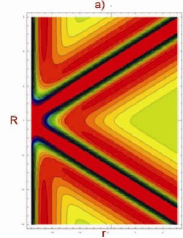
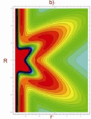
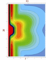
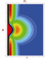
The smooth curves (coordinate reactions) $\Im_{if}$ and ${\Im^{\prime}}_{if}$ in figure connect correspondingly reagent and product asymptotic subspaces in the collinear collisions $A+(BC)$ and $A+(CB)$. It is obvious that in this case the different reaction channels are isolated and there is no interference between them. The illustration of this fact is shown on the example of ab initio PES, termed LSTH, type potential energy surface for reactive system $H+H_{2}$ (see FIG. 5a) Sieg ; Truhl . When the Jacobi angle is fixed $\theta\in(0,\pi)$, going along the curve $\Im_{if}$ or ${\Im^{\prime}}_{if}$ we can’t come to mentioned products subspaces. In other words the exchange reaction channels on the plane $(R,r)$ in this case are closed and this is an universal kinematic property of scattering and doesn’t depend from particles sort (see FIG. 5b-5d).

Refer to caption
Refer to caption
Refer to caption
Refer to caption
Figure 6: Energetic surfaces of reactive system $H+H_{2}$ in the coordinates plane $(r,\theta)$ for different fixing coordinates $R$. It is evident from pictures in the strong interaction region (the region where interactions between all particles are essentially) that there are two potential holes one around the angle $\theta=0$ (or collinear configuration $A+(BC)$) and the second around the angle $\theta=\pi$ (or collinear configuration $A+(CB)$). It is obviously that during the evolution the three body system with big probabilities can fall within first or second hole.
Refer to caption
Refer to caption
Refer to caption
Refer to caption
Figure 7: Energetic surfaces of reactive system $H+H_{2}$ in the coordinates plane $(R,\theta)$ for different fixing coordinates $r$. On these energetic surfaces are generated gradients which push on the three body system to collinear configurations.

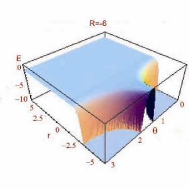
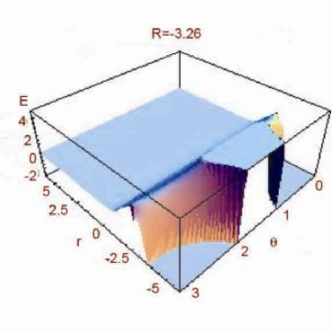
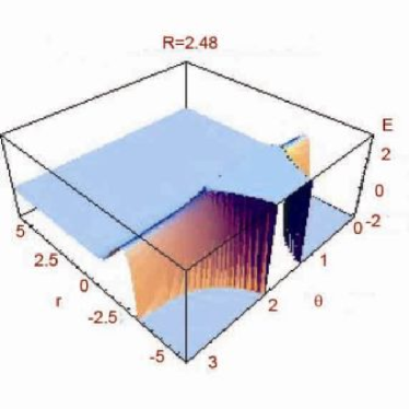
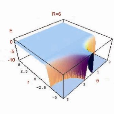
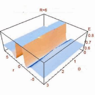
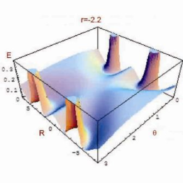
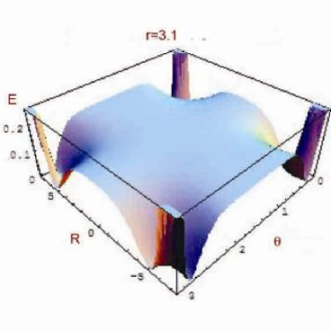
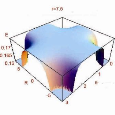
However, in this case the reaction goes out of mentioned plane in $3D$ space (see FIG. 6a-6d and FIG. 7a-7d). As kinematic analysis shows, the $3D$ region, where the probability of reactive scattering processes is concentrated, is essential around the collinear collision plane $(R,r)$. Moreover, this region is compressed to the plan $(R,r)$ as system is evolving along coordinate reaction curve $\Im_{if}$ (or ${\Im^{\prime}}_{if}$) to the asymptotic subspace of products. Recall that all topological properties of reaction surface, which are in Jacobi coordinates system, are conserved in $3D$ NCC system too.

So, the $3D$ NCC system, which is connected with the reaction coordinate curves $\Im_{if}$ or ${\Im^{\prime}}_{if}$, describes uniquely $3D$ part of configuration space, where multichannel scattering process is concentrated.

Appendix B Mass-scaled distances between three-body

For right introducing of NCC system it is necessary to connect the curve of reaction coordinate $\Im_{if}$ in the plan of $(q_{0},q_{1})$ with two equilibrium distances of diatoms of $(in)$ and $(out)$ asymptotic channels. Let us consider the distant between $A$ and $B$ particles in the $(in)$ Jacobi coordinates (see FIG. 1):

$$R_{AB}=\sqrt{R^{2}_{\alpha}-2\rho R_{\alpha}r_{\alpha}\cos\theta_{\alpha}+(\rho r_{\alpha})^{2}},\quad\rho=\frac{m_{C}}{m_{b}+m_{C}},$$ (63)

where indexes which note channels are admitted. After simple transformations taking into account (2) and (3) from (63) we can find:

$$R_{AB}=\sqrt{\lambda^{-2}q_{0}^{2}-2\rho q_{0}q_{1}\cos\theta+\lambda^{2}(\rho q_{1})^{2}}=\lambda^{-1}\sqrt{q_{0}^{2}-2bq_{0}q_{1}\cos\theta+(bq_{1})^{2}}=\lambda^{-1}q_{2},$$ (64)

where $b=\rho\lambda^{2}=\cot\varphi$, and $q_{2}$ is mass-scaled distance between $A$ and $B$ particles. Now we can investigate the asymptotic behavior of mass-scaled distance $q_{2}$. From Eq. (64) with taking into account (5) in the $(in)$ channel (in the limit of $q_{1}^{c}\to q_{eq}^{-}$) may be find:

$$q_{2}\bigl{|}_{\Im_{if}}-q_{0}^{c}=\bigl{(}q_{2}^{c}-q_{0}^{c}\bigr{)}\bigl{|}_{q_{1}^{c}\to q_{eq}^{-}}=-bq_{eq}^{-}\cos\theta.$$ (65)

From which is following that curve $\Im_{if}$ in the reactant $(in)$ channel comes to equilibrium diatom $(BC)$ distance $q_{eq}^{-}$.

Because Jacobi scattering angle which is defined in $(in)$ channel in the $(out)$ channel is limited to zero ( $\theta\to 0$) from (64) and (5) can be find:

$$q_{2}^{c}\bigl{|}_{q_{1}^{c}\to\infty}=q_{0}^{c}-bq_{1}^{c}=q_{eq}^{+},$$ (66)

which is mean that in product $(out)$ channel curve $\Im_{if}$ coming to equilibrium distance $q_{eq}^{+}$ of $(AB)$ diatom.

So, the definition of curve of reaction coordinate $\Im_{if}$ which is defined by formulas (5) and (6) satisfies the aforementioned asymptotic conditions.

Completely note that definition of curve of reaction coordinate $\Im_{if}^{\prime}$ for exchange reaction $A+(CB)\to(AC)+B$ we can find from (5) putting instead of constants $b$ and $q_{eq}^{+}$ constants $(1-b)$ and $\widetilde{q}_{eq}^{+}$ correspondingly, where $\widetilde{q}_{eq}^{+}$ is an equilibrium distance between pair $(AC)$ in the asymptotic channel ($q_{1}^{c}\to+\infty$).

As for the dissociation reaction $A+(BC)\to A+B+C$ it can be described by term of both NCC systems. Only in this case we must remember that Jacobi angle does not limit to zero and can have any value.

Appendix C Calculation of metric tensor in curvilinear reaction coordinates

Let us calculate the transformation between Jacobi scaled and NCC coordinates systems in the plan $(q_{0},q_{1})$. As well known covariant metric tensor defined by:

$$\gamma_{ij}=\sum_{k=0}^{1}\frac{\partial{q_{k}}}{\partial{{x}^{i}}}\frac{\partial{q_{k}}}{\partial{x}^{j}},\qquad\{{x}^{j}\}=(x^{0},x^{1})\equiv(u,v),\quad i,j,k=0,1.$$ (67)

In order to do this, first we calculate the non-diagonal terms. Using (5) and (6), as well as the fact that $x^{0}$ and $x^{1}$ are orthogonal, one can obtain from (67) the following expression:

$\displaystyle\gamma_{01}=\gamma_{10}=-\biggl{(}\frac{dq_{0}^{c}}{d{u}}-v\cos{\phi(u)}\frac{d\phi}{du}\biggr{)}\sin{\phi}+\biggl{(}\frac{dq_{1}^{c}}{d{u}}-v\sin{\phi(u)}\frac{d\phi}{du}\biggr{)}\cos{\phi}$
$\displaystyle=-\frac{dq_{0}^{c}}{d{u}}\sin{\phi(u)}+\frac{dq_{1}^{c}}{d{u}}\cos{\phi(u)}.$ (68)

Requiring orthogonality of the NCC we set $\gamma_{01}=\gamma_{10}=0$, giving:

$$\frac{dq_{0}^{c}}{dq_{1}^{c}}=\cot{\phi{(u)}},$$ (69)

on the curve $\Im_{ij}$. Note that the function $\phi{(u)}$ has a simple geometrical meaning: it corresponds to the angle between the tangential to the reaction coordinate and $q_{1}$. From (69) it is easy to get:

$$\sin\phi(u)=\frac{1}{\sqrt{1+\bigl{(}{dq_{0}^{c}}\bigl{/}{dq_{1}^{c}}\bigr{)}^{2}}},\qquad\cos\phi(u)=\frac{{dq_{0}^{c}}\bigl{/}{dq_{1}^{c}}}{\sqrt{1+\bigl{(}{dq_{0}^{c}}\bigl{/}{dq_{1}^{c}}\bigr{)}^{2}}}.$$ (70)

After derivation $\sin\phi(u)$ by variable $u$ with taking into account (70) one can write:

$$\bigl{(}\sin\phi(u)\bigr{)}_{;\,u}=\cos\phi(u)\,\frac{d\phi}{du}=-\frac{{dq_{0}^{c}}\bigl{/}{dq_{1}^{c}}}{\Bigl{\{}{1+\bigl{(}{dq_{0}^{c}}\bigl{/}{dq_{1}^{c}}\bigr{)}^{2}\Bigr{\}}^{3/2}}}\frac{d}{du}\Bigl{(}\frac{dq_{0}^{c}}{dq_{1}^{c}}\Bigr{)}.$$ (71)

Using equations (5) and (6) from (71) may be find:

$$\bigl{(}\sin\phi(u)\bigr{)}_{;\,u}=-\frac{2a}{\bigl{(}q_{1}^{c}-q_{eq}^{-}\bigr{)}^{3}}\frac{b-a/\bigl{(}q_{1}^{c}-q_{eq}^{-}\bigr{)}^{2}}{b+a/\bigl{(}q_{1}^{c}-q_{eq}^{-}\bigr{)}^{2}}{\biggl{\{}{1+\Bigl{[}b-a/{\bigl{(}q_{1}^{c}-q_{eq}^{-}\bigr{)}^{2}}\Bigr{]}^{2}\biggr{\}}^{-3/2}}},$$ (72)

where symbol $()_{;s}$ is denoted derivation.

The expression for function $\bigl{(}\sin\phi(u)\bigr{)}_{;u}$ correspondingly have a form:

$\displaystyle\bigl{(}\cos\phi(u)\bigr{)}_{;\,u}=-\frac{2a}{\bigl{(}q_{1}^{c}-q_{eq}^{-}\bigr{)}^{3}}\frac{1}{b+a/\bigl{(}q_{1}^{c}-q_{eq}^{-}\bigr{)}^{2}}{\biggl{\{}{1+\Bigl{[}b-a/{\bigl{(}q_{1}^{c}-q_{eq}^{-}\bigr{)}^{2}}\Bigr{]}^{2}\biggr{\}}^{-3/2}}}.$ (73)

For matrix element $\gamma_{00}$ from (67) may be find expression:

$\displaystyle\gamma_{00}=\biggl{(}\frac{\partial{q_{0}}}{\partial{u}}\biggr{)}^{2}+\biggl{(}\frac{\partial{q_{1}}}{\partial{u}}\biggr{)}^{2}=\biggl{(}\frac{dq_{0}^{c}}{d{u}}-v\cos{\phi(u)}\frac{d\phi}{du}\biggr{)}^{2}+\biggl{(}\frac{dq_{1}^{c}}{d{u}}-v\sin{\phi(u)}\frac{d\phi}{du}\biggr{)}^{2}.$ (74)

Substituting the derivatives (72) and (73) into (74) we obtain:

$\displaystyle\gamma_{00}=\bigl{[}1+K(u)v\bigr{]}^{2}\biggl{(}\frac{ds}{du}\biggr{)}^{2},$ (75)

where $K(u)$ is Gaussian curvature of reaction coordinate curve $\Im_{if}$ and $s$ is correspondingly the length along the $\Im_{if}$:

$\displaystyle K(u)=\frac{2a}{\bigl{(}q_{1}^{c}-q_{eq}^{-}\bigr{)}^{3}}\biggl{\{}1+\Bigl{[}b-a/{\bigl{(}q_{1}^{c}-q_{eq}^{-}\bigr{)}^{2}}\Bigr{]}^{2}\biggr{\}}^{-3/2},$
$\displaystyle\biggl{(}\frac{ds}{du}\biggr{)}^{2}=\biggl{\{}1+\Bigl{[}b-a/{\bigl{(}q_{1}^{c}-q_{eq}^{-}\bigr{)}^{2}}\Bigr{]}^{2}\biggr{\}}\biggl{\{}b+a/{\bigl{(}q_{1}^{c}-q_{eq}^{-}\bigr{)}^{2}}\biggr{\}}^{-2}.$ (76)

Note that the Lam$\acute{e}$ coefficient is given by $\eta=\sqrt{\gamma_{00}}$.

We also note that the elements $\gamma_{02}=\gamma_{02}=\gamma_{12}=\gamma_{21}$ vanish. Remind that the second diagonal element $\gamma_{11}$ may be obtained by using (5)-(6) and (67):

$$\gamma_{11}=\biggl{(}\frac{\partial{q_{0}}}{\partial{v}}\biggr{)}^{2}+\biggl{(}\frac{\partial{q_{1}}}{\partial{v}}\biggr{)}^{2}=1.$$ (77)

Thus the metric tensor $\gamma_{ij}$ is diagonal. Finally we note that the covariant tensor is defined as:

$$\gamma^{ij}=B_{ij}\bigl{/}\gamma,\quad\gamma=Det\bigl{(}\gamma_{ii}\bigr{)}=\gamma_{00}\gamma_{11}=\gamma_{00},$$ (78)

where $B_{ij}$ is the algebraic complement to $\gamma_{ij}$.

Appendix D S-matrix contraction by reaction coordinate (intrinsic time) formalism

Between full wavefunctions in the different body-fixed systems the following transformation may be written (see (III.2) ):

$\displaystyle\sum_{\bar{K}}\rho^{-1/2}_{\alpha}{\Phi}^{(\pm)J}_{nj\bar{K}}(u_{\alpha},v_{\alpha},\theta_{\alpha})D^{J}_{\bar{K}K}(\Omega_{\alpha})=\,\sum_{\bar{K}}\rho^{-1/2}_{\beta}{\Phi}^{(\pm)J}_{nj\bar{K}}(u_{\beta},v_{\beta},\theta_{\beta})D^{J}_{\bar{K}K}(\Omega_{\beta}).$ (79)

Next we multiply the equation (79) by the Wigner $D^{J\ast}_{\bar{K}\bar{K}}(\Omega)$-function and integrate, using the volume element $d\Omega=\sin\zeta_{2}\,d\zeta_{1}d\zeta_{2}d\zeta_{3}$. With help of formulas:

$$\int\,D^{J_{1}\ast}_{M_{1}M^{\prime}_{1}}(\zeta_{1},\zeta_{2},\zeta_{3})D^{J_{2}}_{M_{2}M^{\prime}_{2}}(\zeta_{1},\zeta_{2},\zeta_{3})\,d\Omega\,=\frac{8\pi^{2}}{2J_{1}+1}\delta_{J_{1}J_{2}}\delta_{M_{1}M_{2}}\delta_{M_{1}^{\prime}M^{\prime}_{2}}$$

and (25) we get:

$${\Phi}^{(\pm)J}_{njK}(u_{\alpha},v_{\alpha},\theta_{\alpha})=\Bigl{(}\frac{\rho_{\alpha}}{\rho_{\beta}}\Bigr{)}^{1/2}\,\sum_{\bar{K}}d_{\bar{K}K}^{J}(\vartheta){\Phi}^{(\pm)J}_{nj\bar{K}}(u_{\beta},v_{\beta},\theta_{\beta}).$$ (80)

Now we are multiplying the equation (19) on the $(out)$ asymptotic state (21)-(III.2) and integrating it by coordinates $v$ and $\theta$ after which in the limit $u\rightarrow+\infty$ the scattering matrix elements may be found:

$\displaystyle\lim_{u\rightarrow+\infty}\Bigl{\langle}{\Phi}^{(+)J}_{njK}(u_{\alpha},v_{\alpha},\theta_{\alpha}){\Phi}_{n^{\prime}j\,^{\prime}K^{\prime}\,}^{(out)J}(u_{\beta},v_{\beta},\theta_{\beta})\Bigr{\rangle}_{v\theta}=\qquad\qquad\qquad\qquad$
$\displaystyle\sum_{\widetilde{n}\,\widetilde{j\,}\,\widetilde{K}}\emph{S}^{J}_{\widetilde{n}\widetilde{j\,}\widetilde{K}\,\leftarrow\,njK}\,\lim_{u\rightarrow+\infty}\Bigl{\langle}{\Phi}^{(-)J}_{\widetilde{n}\widetilde{j}\widetilde{K}}(u_{\beta},v_{\beta},\theta_{\beta}){\Phi}_{n^{\prime}j\,^{\prime}K^{\prime}}^{(out)J}(u_{\beta},v_{\beta},\theta_{\beta})\Bigr{\rangle}_{v\theta}$
$\displaystyle=\sum_{\widetilde{n}\,\widetilde{j\,}\,\widetilde{K}}\delta_{n^{\prime}\widetilde{n}}\,\delta_{j\,^{\prime}\widetilde{j}}\,\delta_{K^{\prime}\widetilde{K}}\emph{S}^{J}_{\widetilde{n}\widetilde{j\,}\widetilde{K}\,\leftarrow\,njK}=\emph{S}^{J}_{n^{\prime}j\,^{\prime}K^{\prime}\,\leftarrow\,njK}\,.$ (81)

So we found a new expression for the scattering S-matrix elements between $(in)$ and $(out)$ asymptotic states which are defined on different $\alpha$ and $\beta$ surfaces:

$\displaystyle\emph{S}^{J}_{n^{\prime}j\,^{\prime}K^{\prime}\,\leftarrow\,njK}=\lim_{u\rightarrow+\infty}\Bigl{\langle}{\Phi}^{(+)J}_{njK}(u_{\alpha},v_{\alpha},\theta_{\alpha}){\Phi}_{n^{\prime}j\,^{\prime}K^{\prime}}^{(out)J}(u_{\beta},v_{\beta},\theta_{\beta})\Bigr{\rangle}_{v\theta}.$ (82)

Note that in this approach coordinate of translational motion $u$ plays similar role as a usual time in the standard scattering theory and will be called intrinsic time.

Now it is important to find the S-matrix elements form in the one coordinates system $\alpha$ or correspondingly $\beta$.

Putting the expression for overall wavefanction (27) in the (82) we can find:

$$\emph{S}^{J}_{n^{\prime}j\,^{\prime}K^{\prime}\,\leftarrow\,njK}(E)=\lim_{u\to+\infty}\sqrt{\frac{p^{+}_{n^{\prime}j\,^{\prime}}}{p^{-}_{nj}}}\Bigl{<}\sum_{\bar{K}}d_{\bar{K}K}^{J}(\vartheta){\Phi}^{(+)J}_{nj\bar{K}}(u,v,\theta){\Phi}_{n^{\prime}j\,^{\prime}K^{\prime}}^{(out)J}(u,v,\theta)\Bigr{>}_{v_{\beta}\theta_{\beta}}.$$ (83)

Since the angle $\vartheta$ between vectors $\textbf{q}_{0\alpha}$ and $\textbf{q}_{0\beta}$ in the $(out)$ channel (when $u\to+\infty$) is limited to $\pi$ and taking into account that:

$$d_{(\bar{K}-K)}^{J}(\pi)=(-1)^{\bar{K}-K}\delta_{\bar{K}K},$$ (84)

it is easy to get the expression for S-matrix elements:

$$S^{J}_{n^{\prime}j\,^{\prime}K^{\prime}\,\leftarrow\,njK}(E)=\sqrt{\frac{p^{+}_{n^{\prime}j\,^{\prime}}}{p^{-}_{nj}}}\lim_{u\rightarrow+\infty}\Bigl{\langle}{\Phi}^{(+)J}_{njK}(u,v,\theta){\Phi}_{n^{\prime}j\,^{\prime}K^{\prime}}^{(out)J}(u,v,\theta)\Bigr{\rangle}_{v\theta}.$$ (85)

Besides in the expression (85) the coefficient $\sqrt{{p^{+}_{\bar{n}\bar{j}}}/{p^{-}_{nj}}}$ is described flux normalization constant:

$$\sqrt{\frac{p^{+}_{n^{\prime}j\,^{\prime}}}{p^{-}_{nj}}}=\lim_{u\to+\infty}\Bigl{(}\frac{\rho_{\alpha}}{\rho_{\beta}}\Bigr{)}^{1/2}.$$ (86)

In another words we proved that it is possible to represent the full and asymptotic wavefunctions in term of same NCC system without matching between reactant and product channels. It is very important result of developed theory.

So, the matrix elements $S_{n^{\prime}j\,^{\prime}K^{\prime}\,\leftarrow\,njK}(E)$ describe the amplitudes of transition probabilities between the sets of quantum numbers $(njK)$ and $(n^{\prime}j\,^{\prime}K^{\prime})$ correspondingly in the $(in)$ and $(out)$ channels at fixed total energy $E$ and will be called reactive $S$-matrix elements.

Appendix E Solution of classical oscillator problem

Now we turn to investigation of equation (51) with natural boundary conditions (III.4). This equation can be solved with the help of hypergeometric functions. The solution of Eq. (51), which has the form of an incident wave with positive frequency $\omega_{i}>0$ in the $(in)$ channel (when $u\to-\infty$) for a model frequency (52) may be written in the form (see for example BirDev ):

$\displaystyle\sigma_{in}(\tau)=\omega_{i}^{-1/2}\exp\Bigl{\{}i\omega_{+}\tau+i\frac{\omega_{-}}{\lambda\,\,}\ln[2\cosh{(\lambda{\tau})}]\Bigr{\}}\times$
${}_{2}F_{1}\Bigl{[}1-i\frac{\omega_{-}}{\lambda},\,\,\,-i\frac{\omega_{-}}{\lambda};\,\,1+i\frac{\omega_{i}}{\lambda};\,\frac{1}{2}\bigl{(}1+\tanh{(\lambda{\tau})}\bigr{)}\Bigr{]}\stackrel{{\scriptstyle\sim}}{{{}_{\tau\rightarrow-\infty}}}\,\,\omega_{i}^{-1/2}\exp{\bigl{(}i\omega_{i}\tau}\bigr{)},$ (87)

where

$$\omega_{\pm}=\frac{1}{2}(\omega_{f}\pm\omega_{i}),\quad\omega_{i,f}=A_{0}\mp{A_{1}}.$$ (88)

Now we can write the solution of Eq. (51) which satisfies another asymptotic condition in the $(out)$ channel:

$\displaystyle\sigma_{out}(\tau)=\omega_{f}^{-1/2}\exp\Bigl{\{}i\omega_{+}\tau+i\frac{\omega_{-}}{\lambda\,\,}\ln[2\cosh{(\lambda{\tau})}]\Bigr{\}}\times$
${}_{2}F_{1}\Bigl{[}1-\frac{\omega_{-}}{\lambda},\,\,\,-i\frac{\omega_{-}}{\lambda};\,\,1-i\frac{\omega_{f}}{\lambda};\,\frac{1}{2}\bigl{(}1-\tanh{(\lambda{\tau})}\bigr{)}\Bigr{]}\stackrel{{\scriptstyle\sim}}{{{}_{\tau\rightarrow+\infty}}}\,\,\omega_{f}^{-1/2}\exp{\bigl{(}i\omega_{f}\tau}\bigr{)}.$ (89)

Both these solutions are connected with each other by Bogoliubov Bog linear transformations:

$\displaystyle\sigma_{in}(\tau)=C_{1}{\sigma}_{out}(\tau)-C_{2}{\sigma}_{out}^{\ast}(\tau),$ (90)

Coefficients $C_{1}$ and $C_{2}$ are easily calculated, using of properties of hypergeometric functions:

$\displaystyle C_{1}=<\sigma_{in}(\tau)\sigma_{out}{(\tau})>_{\tau}=\Bigl{(}\frac{{\omega_{f}}}{\omega_{i}}\Bigr{)}^{1/2}\frac{\Gamma(1+i\omega_{i}/\lambda)\Gamma(i\omega_{f}/\lambda)}{\Gamma(1+i\omega_{+}/\lambda)\Gamma(i\omega_{-}/\lambda)},$
$\displaystyle C_{2}=-<\sigma_{in}(\tau)\sigma_{out}^{\ast}{(\tau})>_{\tau}=\Bigl{(}\frac{{\omega_{f}}}{\omega_{i}}\Bigr{)}^{1/2}\frac{\Gamma(1+i\omega_{i}/\lambda)\Gamma(-i\omega_{f}/\lambda)}{\Gamma(1-i\omega_{+}/\lambda)\Gamma(-i\omega_{-}/\lambda)}.$ (91)

Recall that similar to (90), the following expression may be written for the solution ${\sigma}_{out}(\tau)$:

$\displaystyle\sigma_{out}(\tau)=C_{1}{\sigma}_{in}(\tau)-C_{2}{\sigma}_{in}^{\ast}(\tau),$ (92)

Now taking into account (90), (E) and (92) for coefficient $C_{1}$ and $C_{2}$ we obtain:

$\displaystyle|C_{1}|^{2}=\frac{\sinh^{2}(\pi\omega_{+}/\lambda)}{\sinh(\pi\omega_{in})\sinh(\pi\omega_{out})},\quad|C_{2}|^{2}=\frac{\sinh^{2}(\pi\omega_{-}/\lambda)}{\sinh(\pi\omega_{in})\sinh(\pi\omega_{out})}.$ (93)

Finally from (93) we can find the normalization expression:

$\displaystyle|C_{1}|^{2}-|C_{2}|^{2}=1.$ (94)

So, taking into account (E) and (93), we get the exact solution of Eq. (51), which we must use for future analytical computations, in the form (90).

References

  • (1) G. C. Schatz and A. Kuppermann, J. Chem. Phys., 65, 4642 (1976); ibid. 65, 4668 (1976).
  • (2) A. Kuppermann, in Theoretical Chemistry, Vol.6, Part A; Theory of Scattering: Papers in Honour of Henry Eyring, D. Henderson, ed., (Academic Press, New York, 1981), p.79.
  • (3) D. E. Manolopoulos and D. C. Clary, Quantum calculations on reactive collisions, Annual Rep. C, The Royal Soci. of Chemistry, 95 (1989).
  • (4) P. Honvault and J. M. Launay, J. Chem. Phys., 114, 1057 (2001).
  • (5) S. C. Althorpe, J. Chem. Phys., 114, 1601 (2001).
  • (6) S. K. Gray, G. G. Balint-Kurti, G. C. Schatz, J. J. Lin, X Liu, S. Harich and X. Yang, J. Chem. Phys., 113, 7330 (2000).
  • (7) L. M. Delves, Nucl. Phys., 9 391 (1959); 20 275 (1960).
  • (8) G. C. Schatz, Chem. Phys. Lett. 150, 92 (1988).
  • (9) W. H. Miller and B. M. D. Jansen op der Haar, A new basis set method of quantum scattering calculations, J. Chem. Phys., 86, 6213 (1987).
  • (10) M. Baer and D. J. Kouri, Phys. Rev. A., 4, 1924 (1971); J. Chem. Phys., 56, 4840 (1972); J. Math. Phys., 14, 1637 (1973).
  • (11) M. Baer, Theory of Chemical reaction Dynamics, V 1, CRC Press, Inc. Boca Raton, Florida, 234 (1985).
  • (12) R. Kosloff and D. Kosloff, J. Phys. Chem. 79, 1823 (1983); R. Kosloff, Time-dependent quantum-mechanical methods for molecular dynamics, J. Phys. Chem. 92, 2087 (1988).
  • (13) G. G. Balint-Kurti, Wavepacket theory of photodissociation and reactive scattering, Adv. Chem. Phys., 128, 244 (2003).
  • (14) G. Nyman and Yu Hua-Gen, Quantum theory of bimolecular chemical reactions, Rep. Prog. Phys. 63, 1001 (2000).
  • (15) D. E. Manolopoulos and M. H. Alexander, J. Chem. Phys., 97, 2527 (1992).
  • (16) M. Yang, D. H. Zhang and S-Y. Lee, J. Chem. Phys., 117, 9539 (2002).
  • (17) H-G. Yu and G. Nyman, J. Chem Phys. 112, 238 (2000).
  • (18) R. A. Marcus, J. Chem. Phys., 45, 4493 (1966); R. A. Marcus, J. Chem. Phys., 49, 2610 (1968).
  • (19) J. Light, Adv. Chem. Phys., 19, 1 (1971).
  • (20) R. B. Walker, J.C. Light and A. Altenberger-Siczek, J. Chem. Phys., 64, 1166 (1976).
  • (21) F. W. Frank and J.C. Light, J. Chem. Phys., 90, 265 (1988).
  • (22) E. B. Stechel, F. Webster and J. C. Light, J. Chem. Phys. 88, 1824 (1988).
  • (23) J. C. Light and A. Altenberger-Siczek, J. Chem. Phys. 90, 265 (1988); J. Chem. Phys. 90, 300 (1988).
  • (24) W. H. Miller, N. C. Handy and J. E. Adams, J. Chem. Phys., 72, 99 (1980).
  • (25) G. D. Billing, Chem. Phys., 277, 325 (2002).
  • (26) C. Coletti and G. D. Billing, Phys. Chem. Chem. Phys., 1, 4141 (1999).
  • (27) A. Koch and G. D. Billing, J. Chem. Phys., 107, 7242 (1997).
  • (28) G. D. Billing, Mol. Phys., 89, 355 (1996).
  • (29) A. V. Bogdanov, A. S. Gevorkyan and G. V. Dubrovskiy, Tech. Phys. Lett., 20 N9, 698 (1994).
  • (30) A. S. Gevorkyan, Rep. NAS Armenia, 95, N3, 214 (1995).
  • (31) A. S. Gevorkyan, Dissertation of the Dr.Sci., Microscopic Models of Collisions and Relaxations in The Dynamics of Chemical Reacting Gas, p 275 (2000) (S.Un.St-P.), St. Petersburg (Russia).
  • (32) F. T. Smith, J. Math. Phys., 3, 735 (1962).
  • (33) A. R. Edmonds, Angular Momentum in Quantum Mechanics , Princeton University Press, Princeton, New Jersey, (1960).
  • (34) R. N. Zare, Angular Momentum, Understanding Special abstracts in Chemistry and Physics, John Wiley and Sons, N. York, 349 (1986).
  • (35) R. T. Pack and G.A. Parker, Quantum reactive scattering in three dimensions using hyperspherical (APH) coordinates. Theory, J. Chem. Phys., 87, 3888 (1987).
  • (36) G. L. Hofacker, Quantentheorie Chemischer Reactionen, Natarforschung, 189, 607 (1963).
  • (37) R. B. Walker, J. C. Light and A. Altenberger-Siczek, Chemical reaction theory for asymetric atom-molecular collisions, J. Chem. Phys., 64, 1166 (1976).
  • (38) R. G. Newton, Scattering Theory of Waves and Particles, McGraw-Hill book Comp., N. York, (1966).
  • (39) M. L. Goldbereger and K. M. Watson, Collision Theory, Jhon Wiley and Sons. INC. New York-London-Sydney, (1964).
  • (40) A. S. Davydov, Quantum Mechanics, trans. by D. ter Haar, Pergamon, N. York, copyright (1965).
  • (41) M. E. Rose, Elementary Theory of Angular Momentum, John Wiley and Sons, N. York, (1957).
  • (42) G. G. Balint-Kurti in International Review of Scince, Series II, Vol 1 page 286, Eds. A. D. Buckingham and C. A. Coulson, Butterworths, London (1975).
  • (43) J. C. Light and R. B. Walker, J. Chem. Phys., 65, 4272 (1976).
  • (44) W. H. Miller, J. Chem. Phys., 49, 2374 (1967).
  • (45) W. A. Lester, Jr., in Modern Theoretical Chemistry, Vol. 1, ed. W.H. Miller, Plenum Press, New York, 1976.
  • (46) W. H. Miller, Annu. Rev. Phys. Chem., 41, 245 (1990).
  • (47) I. A. Malkin and V. I. Man’ko, Dynamic symmetry and coherent states of quantum system, [Nauka, Moscow in Russian] 319, 1979.
  • (48) P. Gamiz et al., J. Math. Phys., 12, 2040 (1971).
  • (49) R. C. Witten and F. T. Smith, J. Math. Phys., 9, 1103 (1968); R.C. Witten, J. Math. Phys., 10, 1631 (1989).
  • (50) V. V. Dodonov, I. A. Malkin and V. I. Mal’ko, Phys. Lett., 51 A, 230 (1975).
  • (51) H. Bateman and A. Erd$\acute{e}$lyi, Higher Transcendental functions, MC Graw-Hill Book Comp, V. 2, 1953.
  • (52) N. N. Lebedev, Special functions and its application, [ Fizmathgiz, Moscow in Russian, (1963)].
  • (53) K. Husimi, Prog. Theor. Phys., 9 381 (1953).
  • (54) N. D. Birrell and P. C. W. Davies, Quantum Fields In Curved Space, Cambridge Univ. Press, 1982.
  • (55) N. N. Bogolubov, Sov. J. of Exper. and Theor. Phys., 34, 58 (1958).
  • (56) P. Siegbahn and B. Liu, J. Chem. Phys., 68, 2457, 1978.
  • (57) D. G. Truhlar and C. J. Horowitz, J. Chem. Phys., 68 2466 (1978); ibid, J. Chem. Phys., 71 6258 (1987).