Non-linear model equation for three-dimensional Bunsen flames
Abstract
The non linear description of laminar premixed flames has been very successful, because of the existence of model equations describing the dynamics of these flames. The Michelson Sivashinsky equation is the most well known of these equations, and has been used in different geometries, including three-dimensional quasi-planar and spherical flames. Another interesting model, usually known as the Frankel equation, which could in principle take into account large deviations of the flame front, has been used for the moment only for two-dimensional expanding and Bunsen flames. We report here for the first time numerical solutions of this equation for three-dimensional flames.
Keywords: laminar reacting flows
Bruno Denet
IRPHE 49 rue Joliot Curie BP 146 Technopole de Chateau Gombert 13384 Marseille Cedex 13 France
submitted to Physics of Fluids
1 Introduction
The Michelson Sivashinsky equation, or simply Sivashinsky equation, depending on the author [1], is a good example of a non linear model equation that has obtained results far beyond any expectations. While originally derived for flames with a low heat release (which are rather rare indeed, since in typical flames the burnt gases have a temperature five times higher than the fresh gases) this equation has succeeded in providing a qualitative description of the dynamics, even for large heat release. This equation has been used for fronts in different geometries (planar on the average [2], expanding flames[3], oblique flames [4]), but with always the limitation that the deviation (actually the variation of the slope) from the unperturbed geometry must be relatively small, and that the front has to be described by a function (of the lateral coordinate, of an angle …)
Another possible description [5] has been proposed in 1990 by Frankel and does not suffer from these drawbacks, i.e. its formulation is coordinate-free, with no privileged direction. It was pointed out to the author by one referee that an approach similar to Frankel’s (using a potential approximation for the flame generated flow field) had already been used in a 1982 article by Ghoniem, Chorin and Oppenheim [6], which could justify changing the name of the equation (usually called Frankel equation). However, contrary to [5], the front was not described in a lagrangian way by a set of markers, but was calculated using a SLIC method [7]. Another difference is that turbulence was described in [6] with vortex methods. The two approaches are thus not completely equivalent. However, it is true that several aspects of the work of Frankel were used by other authors before the 1990 paper (see for instance [8][9]).
In [5], the flow is supposed potential everywhere, fresh and burnt gases, and the problem is transformed into an integro-differential equation involving Green’s functions and the position of the front. This may at first seem completely ridiculous; after all, it is known that for large heat release, vorticity is generated at the front and has to be present in the burnt gases, even if the flow is potential in the fresh gases. But actually, this approximation is close to the low heat release limit of the Sivashinsky equation, and it has been shown in the 1990 Frankel article (a very important point of this paper) that this equation reduces to the Sivashinsky equation for plane on the average and circular flames. Surprising as it may seem, the success of the Sivashinsky equation is actually a (qualitative) success of the potential approximation. However, contrary to the Sivashinsky equation, the Frankel equation has not been for the moment derived rigorously from an expansion in powers of the density ratio starting from the hydrodynamic equations. Higher order expansions in power of the density ratio have lead in the plane case to the derivation of extensions of the Sivashinsky equation [13] (see also [14]). An alternative method has been proposed [12] , based on a weak-nonlinearity approximation. This approximation has been criticized in [13].
The good qualitative agreement of the potential model with experiments (see for instance the comparison in [10] or the figures of the current article) is thus less surprising: the same behavior is seen in the related Sivashinsky equation case. Naturally, the author does not claim that the agreement is quantitative, as the potential approximation is well-known to change the linear growth rate of the Landau instability [11]. For large heat release, the potential model does not satisfy the correct conservation laws at the front, particularly the pressure jump condition, which explains this discrepancy.
In this article, however, we will limit ourselves to the potential model. Numerical solutions of this equation for two dimensional flames are much more difficult than in the Michelson Sivashinsky case, where typically periodic boundary conditions and fast Fourier transforms are used. In the coordinate-free case, the front, which is a line, is discretized with different marker points, which move because of the fluid velocity and the flame speed. Nevertheless, simulations of this equation have appeared in the expanding flame [16][17] [18][19] and the Bunsen burner case[10]. But for the moment no numerical solution of this equation has been obtained for three dimensional flames, where the front has to be described by a surface and not a line. On the contrary, the Michelson Sivashinsky equation has been solved numerically for these flames (see for instance planar flame solutions without and with gravity [2] [20] and a recent paper on spherical flames[21])
In this article we will show the first numerical solutions of the Frankel equation for three dimensional flames, in the Bunsen burner geometry. The equation will be presented, along with some technical details of the numerical solution. Then results for flames with different forcings and for polyhedral flames will be shown.
2 Model and numerical method
Let us first recall some notations. The flame velocity relative to premixed gases will be noted ( and will have the constant value in all the simulations presented in this article) . If we define the density of fresh gases, the density of burnt gases, is a parameter measuring gas expansion ( without exothermic reactions, being close to for large gas expansion). This difference in density between fresh and burnt gases is the main cause of the Darrieus-Landau instability of premixed flames. We use in this article an equation relative to fresh gases, in the Bunsen burner geometry, as in [10], contrary to the original article [5], where the equation was written relative to burnt gases for the case of an expanding flame. The unburnt gases are injected at the velocity . We will consider in Section 3 that is constant in space and that the flame is attached on a circle (i.e. we define points on this circle that do not move during the simulation). In Section 4, on the contrary, we shall see that in order to obtain the polyhedral flames observed experimentally, a boundary layer has to be considered.
is the mean curvature at a given point on the flame , is a constant number proportional to the Markstein length, is the normal vector at the current point on the front, in the direction of propagation. After some calculations similar to [5], an evolution equation is obtained, valid for an arbitrary shape of the front, which is here a surface, contrary to [10], where it was only a line.
| (1) |
This equation gives the value of the normal velocity on the front as a sum of several terms, the laminar flame velocity with curvature corrections, the velocity of the incoming velocity field and an induced velocity field (all the terms where appears) which contains an integral over the whole shape (indicated by the subscript in the integral ). This integral is a sum of electrostatic potentials.
The term is a potential velocity field (continuous across the flame) added to the equation in order to satisfy the boundary conditions. Here the condition is simply that
at the injection location, where is parallel to , so that is given by the same type of integral as , but over the image of the front (see [10]), which is a front symmetric of the real flame in the symmetry (actually we have chosen in order to prevent problems from occurring when a front crosses its image)
When the velocity is obtained from equation (1), the marker points which define the surface are moved :
where denotes the position of the current point of the front.
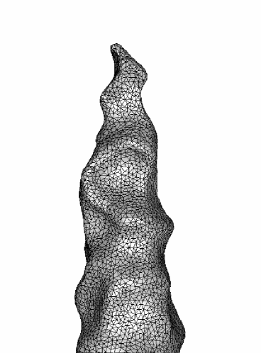
The different marker points of the surface are linked by triangles. A LGPL C library, gts [22] written by Stéphane Popinet, has been used to describe the triangulated surface, perform the integrals in equation (1), and calculate the mean curvature and the normal at any given point. The calculation of the curvature is done by a method proposed in [23]. Let us note that gts itself is implemented using glib, a well-known general purpose library that is also used directly from the author’s program in order to manipulate lists and hash tables. A zoom of a surface shown later (from a different angle) in Figure 3 (right part of the figure) can be seen in Figure 1. As we use a large number of points, typically , the different points cannot be seen if the whole mesh is shown.
Problems typically encountered in Lagrangian descriptions of two-dimensional flames as discontinuities [24] [25] are also present here. First of all, there is a need to adapt the mesh, adding and removing points where necessary. As a result, the type of algorithm used here is inherently noisy, and the noise is higher when there is a rapid time variation. On the other hand, the spatial precision of these Lagrangian descriptions is generally higher than for Eulerian methods, but there is the problem of self-intersections, which occur very often and must be accounted for. One of the interest of this article is to show that it can be done even for three-dimensional flames.
As in [24], we perform the reconnections after the intersection has taken place: we first detect the triangles that self-intersect (this is actually a gts function, which is performed in an efficient way), then these triangles are removed from the surface (except on the boundary). We also remove triangles which are not connected anymore to the main surface after the first triangle removals. At this stage, the surface has one or more holes. We detect the contours of the different holes, and construct small surface patches which are added to the main surface. At this stage, the surface has no hole left, but the patches can have normals oriented in the wrong direction. In order to get a common orientation for the whole surface, we traverse the surface starting from the boundary, looking in a recursive way at each neighbor of a given triangle in order to ensure that the orientation of the whole surface is compatible.
In the simulations that will be presented, we remove pockets created during self-intersections, but actually it would have been very simple to keep pockets with a sufficient number of points. We have programmed a function splitting a surface in its connex components, which are then sorted according to their number of points. Instead of keeping only the main surface (with the largest number of points), it would have been only a matter of two lines of code to apply a different criterion. But the previous experience of the author with two-dimensional flames described in a Lagrangian way has shown that the formation of pockets is generally not very important, except occasionally and for very special forcings. But it is important to discard very small pockets, which can produce all kind of disagreements: further (absolutely unrealistic) splitting of small pockets which forces to reduce the time step, and global inversion of the normal of a small pocket, which actually would have collapsed had the time step been smaller. For real flames naturally, the flame speed is higher when two fronts are very close, which let these small pockets disappear quickly.
Another problem of these simulations, once the intersections are under control, is that the calculations of the integral in equation (1) is very expensive, if done exactly. The problem is exactly an N-body problem (coulombian interaction), where an exact solution for points, is proportional to . As has been already done in a combustion context [17], it is possible to use approximate algorithms which reduce the number of operations. The author himself had always used the exact algorithm when solving the potential model for two-dimensional flames, but the extra dimension has forced him to look at alternatives. There are two main approximate algorithms for the N-body problem. The Greengard and Rokhlyn algorithm [26] (fast multipole expansion) approximates the field by a multipole expansion, the algorithm is but the prefactor is very high. We have preferred to use the Barnes Hut algorithm [27] which is . The idea of this algorithm is to represent the field at a given point by the action of a list of masses, where masses sufficiently far are concatenated in order to provide a good approximation of the field, the masses at the different levels being organized in a tree. The source code of this algorithm can be found in Joshua Barnes’ web site [28].
3 Flames in the presence of forcing
We consider here Bunsen burner flames, with position of the flame imposed on the boundary, i.e. the boundary point must be on a circle of radius (in all the simulations, the value will be chosen) with a value ( is the vertical coordinate). Other boundary conditions will be considered in section 4. In a first step, we would like to show that the three-dimensional Frankel equation contains effects qualitatively similar to those observed with the two-dimensional version in the same geometry [10]. The last article contained evidence of the amplification and saturation of cells created by the Darrieus-Landau instability, which were convected toward the tip of the flame by the incoming flow. Furthermore, a repulsion effect of the side of the flame where forcing was imposed on the other side was observed in the simulations. This effect was very close to the experimental observations of [29]. Here, instead of having a two-dimensional geometry, i.e. a very long rectangular Bunsen flame where the forcing is the same on the long side, we have the usual round burner Bunsen flame.
Let us impose a localized forcing on the flame. We take a sinusoidal forcing, where a term is added to the normal velocity, in a small window , being the polar angle. We take the value which is rather high, but allows to form several wavelengths on the flame. The other parameters are , , . The last parameter and the radius will have the same value in all the simulations presented. The time step is and will keep the same value in all the simulations. This value of the time step is chosen to keep the self-intersections occurring on the front simple. If the time step is too high, very large self-intersections can occur at each time step close to the tip and the precision of the lagrangian description becomes low. We obtain a situation presented in Figure 2. This figure contains three flames. Actually, we had some difficulties in producing different figures of flames with the same scale, so we have included several flames in the same figures. This also makes comparisons easier. The two flames on the left are the same, but seen from a different angle, and correspond to a flame soon after the perturbations produced by the Darrieus-Landau instability reach the tip. If one looks first at the middle image, it can be seen that the sinusoidal forcing is very localized and produces a small perturbation close to the base of the Bunsen flame. But this perturbation develops, is amplified because of the Landau instability, is convected toward the tip and extends laterally, which was of course not observed in two-dimensional experiments and simulations. It is also to be noted that the cells produced by the instability, once sufficiently developed, have a geometry very close to the hexagonal cells well-known in the planar on average configuration. However, when the cell is near the tip, this hexagonal shape becomes less apparent and the cell can be closer from a rectangle.
If one looks now at the side view of the same flame (left of Figure 2), the repulsion effect of the side submitted to perturbations on the other seen in two-dimensional configurations is also present here. As a consequence, there is a slow deflection of the unperturbed side toward the right. This repulsion effect was explained qualitatively by an electrostatic analogy in [10] (let us remember that the model used here is potential). But here this deflection seems smaller, and is seen clearly only when the lateral extension of the perturbations is sufficiently large. Actually, the two-dimensional situation corresponds to a lateral extent infinite in the transverse direction, which explains why in the three-dimensional case, a large lateral extent is needed to obtain the same effect.
The third flame image (right of Figure 2), is a flame with the same physical parameters, but some time later. This flame is higher (the height of the flame fluctuates typically in this way during the temporal evolution). But the main effect is that two cells are merging close to the tip. Apparently, the way we have imposed the forcing does not produce absolutely regular cells, possibly because the forcing zone is too extended. It has happened that one cell had a smaller amplitude close to the base of the flame, and during its translation toward the tip, its amplitude and longitudinal extension have slowly reduced, and now clearly this cell (second cell from the tip, which is very small) is being captured by the third cell, which is very large. This cell merging is absolutely typical of the Landau instability and is well known in the planar configuration, where it helps produce the one-cell flame obtained for every domain size in the Michelson-Sivashinsky equation. Actually, for very large flame height, self-similar mergings have been predicted theoretically [14] [4].
After this study of the effect of a sinusoidal forcing on the flame, we are now interested in the effect of a white noise forcing applied at the base of the flame (sufficiently far from the boundary to prevent problems). To be specific, we have added to the normal velocity at points where a term , where is a random number chosen between and . The white noise is different at each time step and at each point of the mesh. Because the noise is not correlated in space and time, the amplitude must be taken much higher than in the sinusoidal case (a lot of the wavelengths generated by this white noise are quickly damped by diffusion and we wanted to produce a very perturbed flame).
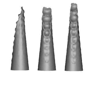
The result of this white noise is shown in Figure 3. We present also here two flames. The flame on the left is a totally unstationary flame obtained soon after the first perturbations reach the tip. The physical parameters are , , and as usual .The initial condition of this calculation was a stationary, unperturbed flame, with slightly different parameters. Starting from the base of the flame, the fine grained perturbations directly caused by the white noise are first seen. Then these perturbations develop because of the instability, leading to cells where this time, it is difficult to recognize any hexagon. Then as in the sinusoidal case, the wavelength of the cells increase because of cell merging. These mergings do not necessary happen in the same way as the one in Figure 2, where a small cell was swallowed by a large one. More symmetrical situations are also possible, where the separation between cells disappear with both cells having approximately the same size. Finally, when the tip is approached, the perturbations organize in order to produce a sinuous shape.
This kind of sinuous shape was also observed for two-dimensional flames [10], and an explanation was proposed. But this sinuous character becomes smaller for typical flames obtained later. We have an example of one typical flame in the right part of the figure. The forcing zone, first cells, wavelength increase and finally sinuous zone can also be seen. It must be admitted however that the flame is much less sinuous than the flame on the left. The main cause of this difference is that as the perturbations develop, the flame height becomes smaller, which can be observed when one compares the two flames in the figure. We can also insist on the three-dimensional structure of the sinuous zone to just say that the shape is almost never truly helical (the author was thinking at the beginning of this work that it was the natural generalization of the sinuous two-dimensional shape, but this is apparently not the case). Before closing this section, one last word, even if we have not performed simulations of turbulent flames, the two flames of Figure 3 can give us some hope that it can be done with the current three-dimensional model. But naturally, it would be very expensive, since it is necessary to either simulate or generate a substitute of turbulent flow. Future growth in computer power will help, the computations of this article being done on a relatively standard PC (2.8 Ghz Pentium 4). It must be noted that the flame lagrangian surface solver used in this article fits naturally with a lagrangian description of vorticity.
4 Polyhedral flames
In the previous section, the positions of the boundary points were imposed and the injection velocity was constant. This is a reasonable approximation of a flame with a very small boundary layer. In this section however, we are interested in polyhedral flames, which are well-known experimentally, see for instance [30]. A theoretical (and experimental, but we will be mainly interested in the theoretical part) article has appeared some time ago [30] on this subject. The polyhedral flames were described by using a modified version of the Kuramoto-Sivashinsky equation, i.e. making the assumption that the instability was of thermal-diffusive origin. This type of model was able to produce polyhedral flames, which is the way cellular flames look like in the Bunsen burner geometry (the following figures show these type of flames). However, with the boundary conditions used in the previous section, we have not been able to produce polyhedral flames, although we have not made an extensive search, for a lot of parameters (the calculations for three-dimensional flames are expensive).
So we are faced with a problem. It would not be a nice situation to conclude that the thermal diffusive instability gives more realistic results than the hydrodynamic one, as the author, among others, has claimed in different papers that the hydrodynamic mechanism is the most realistic. And although not everyone agrees even now, a common belief seems to be that the thermal diffusive mechanism could only account for special cases, like lean hydrogen flames. This is probably why the experiments in [31] were performed with hydrogen.
Before concluding that the hydrodynamic model does not contain polyhedral flames, there is another thing different in [31] from the simulations of the previous section : the boundary conditions. In [31], the vertical position of the boundary points was not imposed, and a flame-holder term was added, following Buckmaster [32], to the Kuramoto-Sivashinsky equation, in order to modelize attraction of the flame to the burner rim.
So let us just apply here these same conditions. However, we shall not apply these conditions unmodified, as we have a slight problem. The vertical coordinate on the boundary is fixed by an equilibrium between the injection velocity, supposed constant everywhere, and the flame-holder term (and also the integral terms in equation 1). As a result we have found, and actually it can be seen in the original article, that the stationary position of the flame is very far from the flame holder. We propose here, in order to describe flames stabilized close to the injection zone, to shift this stationary position toward the flame holder by including the fact that there is a boundary layer, and that as a result the injection velocity close to the boundary is much smaller than in the middle of the tube.
We use the following formula for the injection velocity:
| (2) |
where is the injection velocity at the center of the tube, and are constant coefficients. . The first exponential term is there to describe the boundary layer. The term is the flame holder term used in [31]. The exponential variation with is the one used in this paper, with coefficient controlling the stiffness and width of the boundary layer (proportional to the inverse of the width). Furthermore, contrary to the previous section, just on the boundary, the and coordinates keep the same values, but not the coordinate, which is free to move, being actually computed as a mean value over the neighbors.
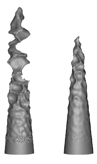
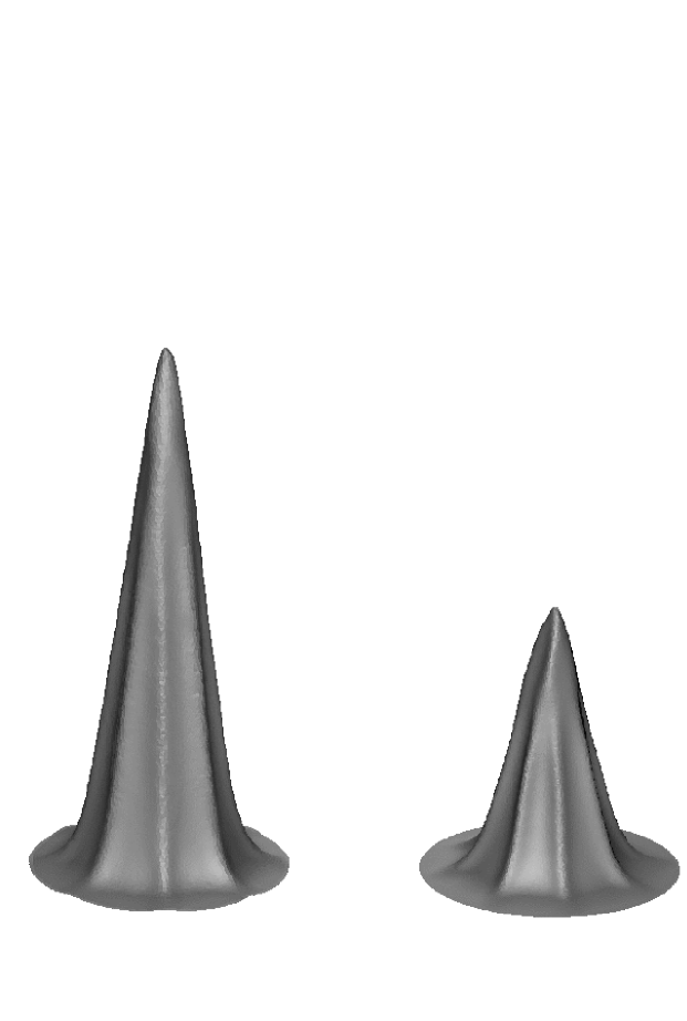
In Figure 4, we show that these modifications of the boundary conditions succeed in making polyhedral flames possible with the Frankel equation. So what is actually important for these flames is not the mechanism in itself, hydrodynamic or thermal-diffusive, but what happens close to the boundary, boundary layer, flame holder term. Actually two flames can be seen in Figure 4 with parameters , , , ,, (left) and (right). These parameters only differ in the injection velocity, showing that, as also observed in the thermal-diffusive case, this parameter does not significantly change the cellular structure of the flame. The eight cells left solution was obtained by taking as initial condition a flame with no cell, but the eight cells solution on the right was actually obtained starting from the solution on the left, and apparently this solution is never completely stationary, as seen in the Figure.
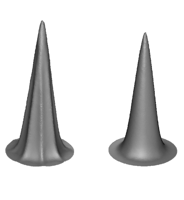
In [31], it was also observed that the parameter , was more important than , and leads to a well-defined transition. As is increased, the flame is no more cellular. This is also the case here in the hydrodynamic case, see Figure 5, where two flames are shown, the one on the left with (same flame as in Figure 4, left) , and on the right with , all the other parameters being the same. It can be seen that although this increase in succeeds in smoothing the flame, the typical values achieving this result are very high. We have not searched the precise value of the bifurcation, but for instance the flame is still weakly cellular with . This very high value has the consequence that the flame is closer from the injection (and above all, closer for a longer distance from the boundary, which is why the flame height is smaller) and very flat close to the boundary, which apparently makes this zone stable. On the contrary, for the small values of used in the other simulations of this article, the role of the flame holder term seems small.
We have also here another parameter, the width of the boundary layer, which did not appear in [31]. In Figure 6, the effect of this parameter is shown. We take (left, large boundary layer), (right, smaller boundary layer) and , , , . Larger boundary layers correspond to more unstable flames, a prediction which can tested experimentally (with some caution, i.e. without changing the flame holder term). This effect could also help explain why it is observed experimentally that larger injection velocities (and smaller boundary layers) lead to flames without any cell. It is unclear at the moment if this effect is sufficient in itself to explain this stabilization.
This effect suggests the following interpretation of the formation of polyhedral Bunsen flames. The cellular perturbations form in the boundary layer. This zone is probably absolutely unstable, and large boundary layers give more time for the perturbations to develop, which thus have a larger amplitude at the exit of this zone. Then the perturbations enter another zone, probably corresponding to a convective instability, and are convected toward the tip. If the perturbations have not reached their amplitude at saturation in the boundary layer, they can continue to amplify during this second phase, leading to cells which appear at a certain distance from the base of the flame, as in Figure 6 (right), where these cells are very weak. These type of solutions have indeed been experimentally observed in [31] (not in their simulations however). If one follows this line of reasoning, the boundary layer width should be compared to typical unstable wavelengths ( most unstable or neutral wavevectors). If this width is much smaller than the unstable wavelengths, the polyhedral flames should be unlikely to be observed. This picture is complicated by the effect of the flame holder term (Figure 5) which probably changes locally the unstable wavelengths, one effect being that flames close to the injection are also closer from their mirror image, which damps the Landau instability.
5 Conclusion
In this article, we have solved for the first time the Frankel equation for three-dimensional flames, in the particular case of the Bunsen burner configuration. This daunting task has been made possible in a reasonable amount of time by using tools (triangulated surface library and N-body problem algorithm) made freely available by their authors, see below the acknowledgments and the references sections. Even with this help, the treatment of intersections is by no means easy, and our program far from perfect. We have tried to explain here the algorithms used to overcome these difficulties. Extensions to other geometries and to turbulent conditions would be interesting.
On the Bunsen burner case, we have shown that this equation can at the same time describe effects absolutely typical of the hydrodynamic Darrieus-Landau instability (Section 3) and also describe polyhedral flames (section 4) in a manner very close to the existing results obtained with the thermal-diffusive instability. We have also emphasized the possible importance of the boundary layer width in this problem.
Acknowledgments : The author would like to thank Stéphane Popinet for the gts library, Joshua Barnes for his implementation of the Barnes-Hut algorithm and Geoff Searby for helpful discussions.
References
- [1] G.I. Sivashinsky. Nonlinear analysis of hydrodynamic instability in laminar flames: Part 1: derivation of basic equations. Acta Astronautica, 4:1117, (1977).
- [2] D.M. Michelson and G.I. Sivashinsky. Thermal expansion induced cellular flames. Combustion and Flame, 48:211, (1982).
- [3] L. Filyand, G.I. Sivashinsky, and M.L. Frankel. On the self-acceleration of outward propagating wrinkled flames. Physica D, 72:110, (1994).
- [4] G. Boury and G. Joulin. Nonlinear response of premixed flame fronts to localized random forcing in the presence of a strong tangential blowing. Combust. Theory Modelling, 6:243, (2002).
- [5] M.L. Frankel. An equation of surface dynamics modeling flame fronts as density discontinuities in potential flows. Phys. Fluids A, 2(10):1879, (1990).
- [6] A.F. Ghoniem, A.J. Chorin, and A K Oppenheim. Numerical modelling of turbulent flow in a combustion tunnel. Phil. Trans. R. Soc., A304:303, (1982).
- [7] W. Noh and P Woodward. Slic (simple line interface calculation). In A. I. v. d. Vooran and P. J. Zandberger, editors, Proceedings, Fifth International Conference on Fluid Dynamics, Berlin, (1976). Springer Verlag.
- [8] M.Z. Pindera and L. Talbot. Flame induced vorticity: the effects of stretch. Proc. Combust. Inst., 21:1357, (1986).
- [9] W.T. Ashurst. Vortex simulation of unsteady wrinkled laminar flames. Combust. Sci. Tech., 52:325, (1987).
- [10] B. Denet. Potential model of a two-dimensional Bunsen flame. Phys. Fluids, 14(10):3577, (2002).
- [11] G.I. Sivashinsky and P. Clavin. On the non linear theory of hydrodynamic instability in flames. J. Phys. France, 48:193, (1987).
- [12] V.V. Bychkov and M.A. Liberman. Dynamics and stability of premixed flames. Physics Reports, 325:115, (2000).
- [13] K.A. Kazakov and M.A. Liberman. Effect of vorticity production on the stucture and velocity of curved flames. Phys. Fluids, 14:1166, (2002).
- [14] G. Boury. Etudes théoriques et numériques de fronts de flamme plissées: dynamiques non-linéaires libres ou bruitées. PhD thesis, Université de Poitiers, (2003).
- [15] V. Bychkov, M. Zaytsev, and V. Akkerman. Coordinate-free description of corrugated flames with realistic density drop at the front. Phys. Rev. E, 68:026312, (2003).
- [16] M.L. Frankel and G.I Sivashinsky. Fingering instability in nonadiabatic low Lewis number flames. Phys. Rev. E, 52(6):6154, (1995).
- [17] S.I. Blinnikov and P. V. Sasorov. Landau Darrieus instability and the fractal dimension of flame fronts. Phys. Rev. E, 53(5):4827, (1996).
- [18] W.T. Ashurst. Darrieus-Landau instability, growing cycloids and expanding flame acceleration. Combust. Theory Modelling, 1:405, (1997).
- [19] B. Denet. Frankel equation for turbulent flames in the presence of a hydrodynamic instability. Phys. Rev. E, 55(6):6911, (1997).
- [20] B. Denet. On non linear instabilities of cellular premixed flames. Combust. Sci. Tech., 92:123, (1993).
- [21] Y. D’Angelo, G. Joulin, and G. Boury. On model evolution equations for the whole surface of three-dimensional expanding wrinkled premixed flames. Combust. Theory Modelling, 4:317, (2000).
- [22] S. Popinet. http://gts.sourceforge.net.
- [23] M. Meyer, M. Desbrun, P. Schröder, and A. Barr. Discrete differential geometry operators for triangulated 2-manifolds http://www-grail.usc.edu/pubs.html. In Vismath 02, Berlin Germany, (2002).
- [24] B. Denet. A lagrangian method to simulate turbulent flames with reconnections. Combust. Sci. Tech., 123:247, (1997).
- [25] J.S.L. Lam, C.K. Chan, L. Talbot, and I.G. Sheperd. On the high resolution modelling of a turbulent premixed open V-flame. Combust. Theory Modelling, 7:1, (2003).
- [26] L. Greengard and V. Rokhlyn. A fast algorithm for particle simulations. J. Comp. Phys., 73:325, (1987).
- [27] J. Barnes and P. Hut. A Hierarchical O(N log N) Force-Calculation Algorithm. Nature, 324:446, (1986).
- [28] J. Barnes. http://www.ifa.hawaii.edu/faculty/barnes/software.html.
- [29] G. Searby, J.M. Truffaut, and G. Joulin. Comparison of experiments and a non linear model equation for spatially developing flame instability. Phys. Fluids, 13(11):3270, (2001).
- [30] S.H. Sohrab and C.K. Law. Influence of burner rim aerodynamics on polyhedral flames and flame stabilization. Combustion and Flame, 62:243, (1985).
- [31] S. Gutman, R.L. Axelbaum, and G.I. Sivashinsky. On Bunsen burner polyhedral flames. Combust. Sci. Tech., 98:57, (1994).
- [32] J. Buckmaster. Polyhedral flames- an exercise in bimodal bifurcation analysis. SIAM J. Appl. Math., 44:40, (1984).
List of Figures
Figure 2 : Flame submitted to a sinusoidal forcing. Parameters , , Left and middle flame: same flame, seen from two angles, showing the development of the Landau instability toward the tip. Right: same flame some time later, showing a merging of two cells close to the tip.
Figure 3 : Flame submitted to a white noise at the base. Left: A flame soon after the instabilities have reached the tip Right: typical flame some time later. Note the sinuous shape of the flames close to the tip. parameters , ,
Figure 4 : Polyhedral flames obtained for two different values of the injection velocity parameters , ,, , (left), (right)
Figure 5: Flames obtained for two different values of the flame holder parameter and other parameters , , ,
Figure 6: Flames obtained for two different values of the boundary layer thickness, (left), (right) other parameters , , ,
Denet, Phys. Fluids
Denet, Phys. Fluids
Denet, Phys. Fluids
Denet, Phys. Fluids
Denet, Phys. Fluids
Denet, Phys. Fluids