Construction of a polarization insensitive lens from a quasi-isotropic metamaterial slab

Abstract

We propose to employ the quasiisotropic metamaterial (QIMM) slab to construct a polarization insensitive lens, in which both E- and H-polarized waves exhibit the same refocusing effect. For shallow incident angles, the QIMM slab will provide some degree of refocusing in the same manner as an isotropic negative index material. The refocusing effect allows us to introduce the ideas of paraxial beam focusing and phase compensation by the QIMM slab. On the basis of angular spectrum representation, a formalism describing paraxial beams propagating through a QIMM slab is presented. Because of the negative phase velocity in the QIMM slab, the inverse Gouy phase shift and the negative Rayleigh length of paraxial Gaussian beam are proposed. We find that the phase difference caused by the Gouy phase shift in vacuum can be compensated by that caused by the inverse Gouy phase shift in the QIMM slab. If certain matching conditions are satisfied, the intensity and phase distributions at object plane can be completely reconstructed at image plane. Our simulation results show that the superlensing effect with subwavelength image resolution could be achieved in the form of a QIMM slab.

I Introduction

About forty years ago, Veselago firstly introduced the concept of left-handed material (LHM) in which both the permittivity $\varepsilon$ and the permeability $\mu$ are negative Veselago1968 . He predicted that LHM would have unique and potentially interesting properties, such as the negative refraction index, the reversed Doppler shift and the backward Cerenkov radiation. Veselago pointed out that electromagnetic waves incident on a planar interface between a regular material and a LHM will undergo negative refraction. Hence a LHM planar slab can act as a lens and focus waves from a point source. LHM did not receive much attention as it only existed in a conceptual form. After the first experimental observation of negative refraction using a metamaterial composed of split ring resonators (SRRs) Smith2000 ; Shelby2001 , the study of such materials has received increasing attention over the last few years. While negative refraction is most easily visualized in an isotropic metamaterial Smith2000 ; Shelby2001 ; Pacheco2002 ; Parazzoli2003 ; Houck2003 , negative refraction can also be realized in photonic crystals Notomi2000 ; Luo2002a ; Luo2002b ; Li2003 and anisotropic metamaterials Lindell2001 ; Hu2002 ; Smith2003 ; Zhang2003 ; Zhou2003 ; Luo2005 ; Thomas2005 ; Luo2006a ; Grzegorczyk2006 have also been reported.

Recently, Pendry extended Veslago’s analysis and further predicted that a LHM slab can amplify evanescent waves and thus behaves like a perfect lens Pendry2000 . He proposed that the amplitudes of evanescent waves from a near-field object could be restored at its image. Therefore, the spatial resolution of the superlens can overcome the diffraction limit of conventional imaging systems and reach the subwavelength scale. The great research interests were initiated by the revolutionary concept. More recently, the anisotropic metamaterials have been proved to be good candidates for slab lens application Smith2004a ; Smith2004b ; Parazzoli2004 ; Dumelow2005 . Although the focusing is imperfect, the substantial field intensity enhancement can readily be observed. In these cases, the anisotropic metamaterials under consideration are characterized by a hyperboloid dispersion relation, and the focusing is restricted to either E- or H-polarized radiation. The recent development in quasiisotropic metamaterial (QIMM) offers us further opportunities to extend the previous work and further predict that both E- and H-polarized waves can be refocused.

The main purpose of the present work is to construct a polarization insensitive lens by a QIMM slab. For shallow incident angles the QIMM slab will provide some degree of refocusing in the same manner as an isotropic LHM slab. We are particularly interested in exploiting polarization insensitive effect. First, starting from the representation of plane-wave angular spectrum, we derive the propagation of paraxial beams in the QIMM slab. Our formalism permits us to introduce ideas for beam focusing and phase compensation of paraxial beams by using the QIMM slab. Next we want to introduce the inverse Gouy phase shift and negative Rayleigh length when waves propagating in the QIMM slab. As an example, we obtain the analytical description for a Gaussian beam propagating through a QIMM slab. We find that the phase difference caused by the Gouy phase shift in vacuum can be compensated by that caused by the inverse Gouy phase shift in the QIMM slab. If certain matching conditions are satisfied, the intensity and phase distributions at object plane can be completely reconstructed at the image plane. Finally, we will discuss what happen when the evanescent wave transmission through the QIMM slab.

II Polarization insensitive metamaterial

Before we consider the polarization insensitive lens, we first analyze what is the QIMM. For anisotropic materials, one or both of the permittivity and permeability are second-rank tensors. In the following we assume that both the permittivity and permeability tensors are simultaneously diagonalizable:

$$\bm{\varepsilon}=\left[\begin{array}[]{ccc}\varepsilon_{x}(\omega)&0&0\\ 0&\varepsilon_{y}(\omega)&0\\ 0&0&\varepsilon_{z}(\omega)\end{array}\right],~{}~{}~{}\bm{\mu}=\left[\begin{array}[]{ccc}\mu_{x}(\omega)&0&0\\ 0&\mu_{y}(\omega)&0\\ 0&0&\mu_{z}(\omega)\end{array}\right],$$ (7)

where $\varepsilon_{j}$ and $\mu_{j}$ are the relative permittivity and permeability constants in the principal coordinate system ($j=x,y,z$). It should be noted that the real anisotropic metamaterial constructed by SRRs is highly dispersive, both in spatial sense and frequency sense Smith2003 ; Smith2004a ; Smith2004b ; Thomas2005 . So these relative values are functions of the angle frequency $\omega$.

Following the standard procedure, we consider a monochromatic electromagnetic field ${\bf E}({\bf r},t)=Re[{\bf E}({\bf r})\exp(-i\omega t)]$ and ${\bf B}({\bf r},t)=Re[{\bf B}({\bf r})\exp(-i\omega t)]$ of angular frequency $\omega$ incident from vacuum into the anisotropic metamaterial. The field can be described by Maxwell’s equations Chen1983

$$\nabla\times{\bf E} = -\frac{\partial{\bf B}}{\partial t},~{}~{}~{}{\bf B}=\mu_{0}\bm{\mu}\cdot{\bf H},$$

$$\nabla\times{\bf H} = \frac{\partial{\bf D}}{\partial t},~{}~{}~{}~{}~{}{\bf D}=\varepsilon_{0}\bm{\varepsilon}\cdot{\bf E}.$$ (8)

The previous Maxwell’s equations can be combined in a straightforward way to obtain the well-known equation for the complex amplitude of the electric field, which reads

$$\nabla\times(\bm{\mu}^{-1}\cdot\nabla\times{\bf E})+\frac{1}{c^{2}}\frac{\partial^{2}{\bf D}}{\partial t^{2}}=0,$$ (9)

where $c$ is the speed of light in vacuum.

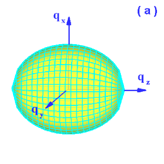
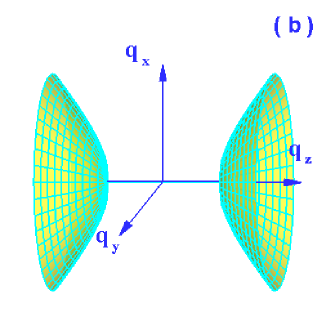
Figure 1: (Color online) (a) The QIMM with ellipsoid wave-vector surface; (b) The QIMM with double-sheeted wave-vector surface.

In the principal coordinate system, Maxwell’s equations yield a scalar wave equation. In free space, the accompanying dispersion relation has the familiar form

$$k_{x}^{2}+k_{y}^{2}+k_{z}^{2}=\frac{\omega^{2}}{c^{2}},$$ (10)

where $k_{j}$ is the $j$ component of the incident wave vector.

We note that the Maxwell’s equations are symmetrical in electric and magnetic fields. So as far as Maxwell’s equations is concerned, what we can do for electricity we can also do for magnetism. To achieve the polarization insensitive effect, we will focus our interesting on the anisotropic metamaterial, in which the permittivity and permeability tensor elements satisfy the condition:

$$\frac{\varepsilon_{x}(\omega)}{\mu_{x}(\omega)}=\frac{\varepsilon_{y}(\omega)}{\mu_{y}(\omega)}=\frac{\varepsilon_{z}(\omega)}{\mu_{z}(\omega)}=C~{}~{}~{}(C>0),$$ (11)

where $C$ is a constant. A careful calculation of the Maxwell’s equations gives the dispersion relation:

$$\left(\frac{q_{x}^{2}}{\varepsilon_{y}\mu_{z}}+\frac{q_{y}^{2}}{\varepsilon_{x}\mu_{z}}+\frac{q_{z}^{2}}{\varepsilon_{y}\mu_{x}}-\frac{\omega^{2}}{c^{2}}\right)\left(\frac{q_{x}^{2}}{\varepsilon_{z}\mu_{y}}+\frac{q_{y}^{2}}{\varepsilon_{z}\mu_{x}}+\frac{q_{z}^{2}}{\varepsilon_{x}\mu_{y}}-\frac{\omega^{2}}{c^{2}}\right)=0,$$ (12)

where $q_{j}$ represents the $j$ component of transmitted wave-vector. The above equation can be represented by a three-dimensional surface in wave-vector space. This surface is known as the normal surface and consists of two shells Chen1983 . Under the condition of Eq. (11), we can find E- and H-polarized waves exhibit the same wave-vector surface. Thus the anisotropic medium also be regard as QIMM Shen2005 ; Luo2006b . Clearly, we can find the dispersion surface has the following two types: ellipsoid and double-sheeted hyperboloid, as show in Fig. 1.

We are currently investigating the possibilities for the manufacture of the QIMM. In fact, it is now conceivable that a metamaterial can be constructed whose permittivity and permeability values may be designed to vary independently and arbitrarily throughout a metamaterial, taking positive or negative values as desired. Hence the permittivity and permeability tensor elements of QIMM can be controlled by modulating the length scale of the SRRs. The permittivity $\varepsilon_{j}(\omega)$ and permeability $\mu_{j}(\omega)$ can be approximated by the Lorentz model. We trust that the QIMM can be constructed, because similar technology has been exploited in anisotropic metamaterial Parazzoli2003 ; Zhou2003 ; Thomas2005 ; Grzegorczyk2006 . In addition, photonic crystals might be a good candidate for constructing a QIMM. The periodicity in photonic crystals is on the order of the wavelength, so that the distinction between refraction and diffraction is blurred. Nevertheless, many novel dispersion relationships can be realized in photonic crystals, including ranges where the frequency disperses negatively with wave vector as required for a negative refraction Notomi2000 ; Luo2002a ; Luo2002b ; Li2003 .

Now we want to enquire: whether E- and H-polarized exhibit the same propagation characteristic. To answer the question we first discuss the transmission of wave vector. We choose the $z$ axis to be normal to the interface, the $x$ and $y$ axes locate at in the plane of the interface. The $z$-component of the transmitted wave vector can be found by the solution of Eq. (12), which yields

$${q_{z}^{E}}=\sigma\sqrt{\varepsilon_{y}\mu_{x}k_{0}^{2}-\varepsilon_{y}\mu_{x}\left(\frac{q_{x}^{2}}{\varepsilon_{y}\mu_{z}}+\frac{q_{y}^{2}}{\varepsilon_{x}\mu_{z}}\right)},$$ (13)

$$q_{z}^{H}=\sigma\sqrt{\varepsilon_{x}\mu_{y}k_{0}^{2}-\varepsilon_{x}\mu_{y}\left(\frac{q_{x}^{2}}{\varepsilon_{z}\mu_{y}}+\frac{q_{y}^{2}}{\varepsilon_{z}\mu_{x}}\right)},$$ (14)

for E- and H-polarized waves, respectively. Here $k_{0}=\omega/c$ is the wave number in vacuum and $\sigma=\pm 1$. This choice of sign ensures that power propagates away from the boundary to the $+z$ direction.

Without loss of generality, we assume the wave vector locate at the $x-z$ plane ($k_{y}=q_{y}=0$). The incident angle of light is given by

$$\theta_{I}=\tan^{-1}\left[\frac{k_{x}}{k_{z}}\right].$$ (15)

The values of refractive wave vector can be found by using boundary conditions and dispersion relations. The refractive angle of the transmitted wave vector or phase of E- and H- polarized waves can be written as

$$\beta_{P}^{E}=\tan^{-1}\left[\frac{q_{x}^{E}}{q_{z}^{E}}\right],~{}~{}~{}\beta_{P}^{H}=\tan^{-1}\left[\frac{q_{x}^{H}}{q_{z}^{H}}\right].$$ (16)

Substituting Eqs. (13) and (14) into Eq. (16), we can easily find that E- and H- polarized waves propagates with the same wave vector or phase velocity.

In the next step, let us discuss the transmission of energy flux. It should be noted the actual direction of light is determined by the time-averaged Poynting vector ${\bf S}=\frac{1}{2}{\bf Re}({\bf E}^{\ast}\times\bf{H})$. For E- and H-polarized waves, the transmitted Poynting vector ${\bf S}_{T}$ is given by

$${\bf S}_{T}^{E}=Re\left[\frac{T_{E}^{2}E_{0}^{2}q_{x}^{E}}{2\omega\mu_{z}}{\bf e}_{x}+\frac{T_{E}^{2}E_{0}^{2}q_{z}^{E}}{2\omega\mu_{x}}{\bf e}_{z}\right],$$ (17)

$${\bf S}_{T}^{H}=Re\left[\frac{T_{H}^{2}E_{0}^{2}q_{x}^{H}}{2\omega\varepsilon_{z}}{\bf e}_{x}+\frac{T_{H}^{2}E_{0}^{2}q_{z}^{H}}{2\omega\varepsilon_{x}}{\bf e}_{z}\right],$$ (18)

where $T_{E}$ and $T_{H}$ are the transmission coefficients for E- and H-polarized waves, respectively. The refraction angle of Poynting vector of E- and H- polarized incident waves can be obtained as

$$\beta_{S}^{E}=\tan^{-1}\left[\frac{S_{Tx}^{E}}{S_{Tz}^{E}}\right],~{}~{}~{}\beta_{S}^{H}=\tan^{-1}\left[\frac{S_{Tx}^{H}}{S_{Tz}^{H}}\right].$$ (19)

Combining Eqs. (16) and (19) we can easily find that E- and H- polarized waves have the same Poynting vector. As for the QIMM slab, the refraction at the second interface can be investigated by the similar procedures.

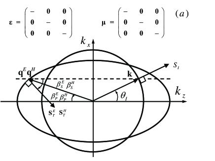
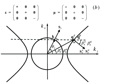
Figure 2: The frequency contours of isotropic and quasiisotropic media: (a) The circle and ellipse represent the frequency contours of vacuum and quasiisotropic media, respectively. Both the wave vector and the energy flow exhibit negative refraction. (b) The circle and hyperbola denote the frequency contours of vacuum and quasiisotropic media, respectively. The wave vector undergoes a positive refraction, while the energy flow undergoes a negative refraction.

By now, we know that E- and H- polarized waves propagate with same wave vector and Poynting vector. It is a significantly different property from general anisotropic media. Note that there is a bending angle between ${\bf q}$ and ${\bf S}$, and therefore ${\bf q}$, ${\bf E}$ and ${\bf H}$ do not form a strictly right-handed or left-handed system in QIMM. Hence it is also different from isotropic media. For this reason, this kind of special anisotropic media is regarded as quasiisotropic. It should be mentioned that if $C<0$ in Eq. (11), E- and H-polarized waves will exhibit the same single-sheeted dispersion relation. While the two polarized waves will undergo different amphoteric refraction, the special anisotropic media cannot be regarded as quasiisotropic Luo2006b .

Now we are in the position to study the negative refraction in the QIMM. Unlike in isotropic media, the Poynting vector in The QIMM is neither parallel nor antiparallel to the wave vector, but rather makes either an acute or an obtuse angle with respect to the wave vector. In general, to distinguish the positive and negative refraction in QIMM, we must calculate the direction of the Poynting vector with respect to the wave vector. Positive refraction means ${\bf q}_{x}\cdot{\bf S}_{T}>0$, and negative refraction means ${\bf q}_{x}\cdot{\bf S}_{T}<0$. From Eqs. (17) and (18) we get

$${\bf q}_{x}^{E}\cdot{\bf S}_{T}^{E}=\frac{T_{E}^{2}E_{0}^{2}q_{x}^{2}}{2\omega\mu_{z}},~{}~{}~{}{\bf q}_{x}^{H}\cdot{\bf S}_{T}^{H}=\frac{T_{H}^{2}H_{0}^{2}q_{x}^{2}}{2\omega\varepsilon_{z}}.$$ (20)

The negative refraction phenomenon is one of the most interesting properties of the QIMM. We can see that the refracted waves will be determined by $\mu_{z}$ for E-polarized incident waves and $\varepsilon_{z}$ for H-polarized incident waves.

Because of the importance of negative refraction in refocusing effect, we are interested in the two types of QIMM, which can formed from appropriate combinations of material parameter tensor elements.
Type I.  In this case all of the $\varepsilon_{j}$ and $\mu_{j}$ are negative. The frequency contour is an ellipse as shown in Fig. 2(a). Here ${\bf k}_{z}\cdot{\bf q}_{z}<0$ and ${\bf q}_{x}\cdot{\bf S}_{T}<0$, so the refraction angle of wave vector and Poynting vector are always negative.
Type II. In this case $\varepsilon_{x}>0$, $\varepsilon_{y}>0$ and $\varepsilon_{z}<0$. The frequency contour is a double-sheeted hyperbola as depicted in Fig. 2(b). Here ${\bf k}_{z}\cdot{\bf q}_{z}>0$ and ${\bf q}_{x}\cdot{\bf S}_{T}<0$. It yields that the refraction of Poynting vector refraction is always negative even if the wave-vector refraction is positive.

As noted above, the Poynting vector will exhibit negative refraction in the two types of QIMM. The negative refraction is the important effect responsible for the slab lens. Hence, the two kind of QIMM can be employed to construct a polarized insensitive lens.

III The Paraxial model of beam propagation

In this section, we consider the slab lens constructed by the QIMM. As depicted in Fig. 3, the QIMM slab in region $2$ is surrounded by vacuum in region $1$ and region $3$. A point source is place the object plane $z=0$. A single ray will pass the interfaces $z=a$ and $z=a+d$ before it reaches the image plane $z=a+b+d$. Let us investigate what happens when the single ray pass through the QIMM slab. Because of the anisotropy the ray incident for different angle will exhibit different image plane.

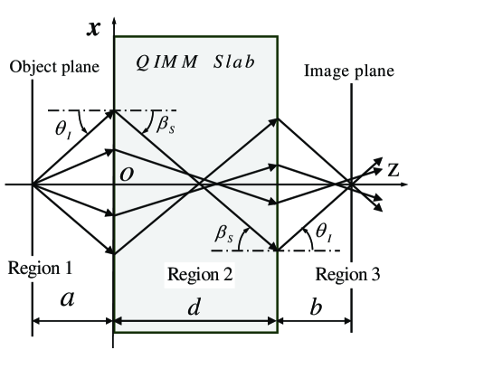
Figure 3: The ray tracing picture showing the focussing by QIMM slab. The QIMM slab is surrounded by vacuum in region 1 and region 3. The solid line and dash-dotted lines are the theoretical objective and focusing planes, respectively.

First, we explore the aberration effect caused by the anisotropic effect. Subsequent calculations of Eq. (19) give the relationship between $\sin{\theta_{I}}$ and $\sin\beta_{s}$ by

$$\sin^{2}\beta_{S}^{E}=\frac{\mu_{x}^{2}\sin^{2}\theta_{I}}{\varepsilon_{y}\mu_{z}^{2}+(\mu_{x}-\mu_{z})\sin^{2}\theta_{I}},$$ (21)

$$\sin^{2}\beta_{S}^{H}=\frac{\varepsilon_{x}^{2}\sin^{2}\theta_{I}}{\mu_{y}\varepsilon_{z}^{2}+(\varepsilon_{x}-\varepsilon_{z})\sin^{2}\theta_{I}}.$$ (22)

Note that the expressions are sightly different from those in conventional uniaxial crystal Dumelow2005 . It is instructive to compare these results with Snell’s law, which for refraction from vacuum into an isotropic medium, gives $\sin\theta_{I}/\sin\beta_{s}=n$, where $n$ represents the refractive index of the refracting medium. Evidently, in the present case we can find the relationship between $\sin{\theta_{I}}$ and $\sin\beta_{s}$ is nonlinear, which is caused by the anisotropic effect $\varepsilon_{x}\neq\varepsilon_{z}$ or $\mu_{x}\neq\mu_{z}$. The nonlinear relationship will result in a significant aberration effect in the image plane, hence the achievable resolution of image is limited.

Next, we want to discuss another aberration effect caused by frequency dispersion. For a certain incident angle, the ray with different frequency will exhibit different image plane as shown in Fig. 4. We assume that both $\varepsilon_{z}(\omega)$ and $\mu_{z}(\omega)$ be approximated by the Lorentz model. The other tensor elements components are approximated as constants. The resonate frequency, plasma frequency, and damping constant are identical in all respects to those utilized in Ref. Thomas2005 . Ignoring the metallic structure, the other tensor elements assume the values of the background material which is dominantly air. Obviously the frequency dispersion of $\varepsilon_{z}(\omega)$ and $\mu_{z}(\omega)$ will place some practical limitations on the resolution of image. Fortunately the limitations can be reduced, if the ray incident at a small angle. The significant effect has be illustrated in Fig. 4. It is interesting to noted that the image distance will slowly vary with frequency in a certain band.

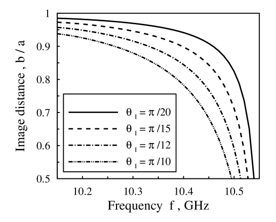
Figure 4: For a certain incident angle, the ray with different frequency $f=\omega/2\pi$ will exhibit different image plane. Note that for smaller incident angles, the QIMM slab will provide some degree of frequency insensitive in a certain GHz band.

Remarkable as the QIMM slab lens is it suffers from some problem: how to cancel the aberration effect? Does the polarization insensitive lens have any use, if the image is not imperfect? The main effect of anisotropy associated with QIMM will limit the resolution of the image. Although the image is imperfect, we trust that the reconstruct effect of intensity and phase in paraxial regime will lead to some potential applications. Such as the QIMM slab can be used to provide phase compensation and beam focusing in cavity resonator. Furthermore, sightly anisotropy in QIMM slab lens can improve the beam parameter. Most importantly, the QIMM can be used to design polarization-insensitive modulators and polarization-insensitive all-optical switching in fiber communication system. Hence it is very desirable to investigate the polarization insensitive effect in paraxial regime.

From a mathematical point of view, the approximate paraxial expression for the field can be obtained by the expansion of the square root of $q_{z}$ to the first order in $|{\bf q}_{\bot}|/q$ Lax1975 ; Ciattoni2000 ; Luo2006c , which yields

$$q_{z}^{E}=\sigma\sqrt{\varepsilon_{y}\mu_{x}}k_{0}-\left(\frac{\sigma\sqrt{\varepsilon_{y}\mu_{x}}k_{x}^{2}}{2\varepsilon_{y}\mu_{z}k_{0}}+\frac{\sigma\sqrt{\varepsilon_{y}\mu_{x}}k_{y}^{2}}{2\varepsilon_{x}\mu_{z}k_{0}}\right),$$ (23)

$$q_{z}^{H}=\sigma\sqrt{\varepsilon_{x}\mu_{y}}k_{0}-\left(\frac{\sigma\sqrt{\varepsilon_{x}\mu_{y}}k_{x}^{2}}{2\varepsilon_{z}\mu_{y}k_{0}}+\frac{\sigma\sqrt{\varepsilon_{x}\mu_{y}}k_{y}^{2}}{2\varepsilon_{z}\mu_{x}k_{0}}\right),$$ (24)

where we have introduced the boundary condition ${\bf q}_{\bot}={\bf k}_{\bot}$. From Eqs. (23) and (24) we can easily find that for shallow incident angles the QIMM slab will provide some degree of refocusing in the same manner as an isotropic LHM. Hence the aberration effect can be cancelled in paraxial beam region. The interesting property allow us to introduce the idea to construct a QIMM slab lens in paraxial beam region.

Equation (9) can be conveniently solved by employing the Fourier transformations, so the complex amplitudes in QIMM for E- and H-polarized beams can be conveniently expressed as

$${\bf E}({{\bf r}_{\bot}},z)=\int d^{2}{\bf k}_{\bot}\tilde{E}({\bf k}_{\bot})\exp[i{\bf k}_{\bot}\cdot{\bf r}_{\perp}+iq_{z}^{E}z].$$ (25)

$${\bf H}({{\bf r}_{\bot}},z)=\int d^{2}{\bf k}_{\bot}\tilde{H}({\bf k}_{\bot})\exp[i{\bf k}_{\bot}\cdot{\bf r}_{\perp}+iq_{z}^{H}z].$$ (26)

Here ${\bf r}_{\perp}=x{\bf e}_{x}+y{\bf e}_{y}$, ${\bf k}_{\perp}=k_{x}{\bf e}_{x}+k_{y}{\bf e}_{y}$, and $e_{j}$ is the unit vector in the $j$-direction.

Substituting Eqs. (23) and (24) into Eq. (25) and (26), respectively, we obtain

$${\bf E}({{\bf r}_{\bot}},z)= \exp(i\sigma\sqrt{\varepsilon_{x}\mu_{y}}k_{0}z)\int d^{2}{\bf k}_{\bot}$$ (27)

$$\times\exp\bigg{[}i{\bf k}_{\perp}\cdot{\bf r}_{\perp}-\left(\frac{\sigma\sqrt{\varepsilon_{y}\mu_{x}}}{2\varepsilon_{y}\mu_{z}k_{0}}k_{x}^{2}+\frac{\sigma\sqrt{\varepsilon_{y}\mu_{x}}}{2\varepsilon_{x}\mu_{z}k_{0}}k_{y}^{2}\right)\bigg{]}\tilde{\bf E}({\bf k}_{\perp}),$$

$${\bf H}({{\bf r}_{\bot}},z)= \exp(i\sigma\sqrt{\varepsilon_{x}\mu_{y}}k_{0}z)\int d^{2}{\bf k}_{\bot}$$ (28)

$$\times\exp\bigg{[}i{\bf k}_{\perp}\cdot{\bf r}_{\perp}-\left(\frac{\sigma\sqrt{\varepsilon_{y}\mu_{x}}}{2\varepsilon_{z}\mu_{y}k_{0}}k_{x}^{2}+\frac{\sigma\sqrt{\varepsilon_{y}\mu_{x}}}{2\varepsilon_{z}\mu_{x}k_{0}}k_{y}^{2}\right)\bigg{]}\tilde{\bf H}({\bf k}_{\perp}).$$

The fields $\tilde{E}({\bf k}_{\bot})$ and $\tilde{H}({\bf k}_{\bot})$ in Eqs. (27) and (28) are related to the boundary distributions of the fields by means of the relation

$$\tilde{{\bf E}}({\bf k}_{\bot})=\int d^{2}{\bf r}_{\bot}{\bf E}({\bf r}_{\bot},0)\exp[i{\bf k}_{\bot}\cdot{\bf r}_{\perp}],$$ (29)

$$\tilde{{\bf H}}({\bf k}_{\bot})=\int d^{2}{\bf r}_{\bot}{\bf H}({\bf r}_{\bot},0)\exp[i{\bf k}_{\bot}\cdot{\bf r}_{\perp}],$$ (30)

for E- and H-polarized beams, respectively. Evidently, Eqs. (29) and (30) are standard two-dimensional Fourier transform Goodman1996 . In fact, after the field distribution in the plane $z=0$ is known, Eqs. (27) and (28) provide the expression of the E- and H-polarized field in the space $z>0$, respectively.

Since our attention will be focused on beam propagating along the $+z$ direction, we can write the paraxial fields as

$${\bf E}({\bf r}_{\perp},z)={\bf A}_{E}({\bf r}_{\perp},z)\exp(i\sigma\sqrt{\varepsilon_{y}\mu_{x}}k_{0}z),$$ (31)

$${\bf H}({\bf r}_{\perp},z)={\bf A}_{H}({\bf r}_{\perp},z)\exp(i\sigma\sqrt{\varepsilon_{x}\mu_{y}}k_{0}z),$$ (32)

where the field $A({\bf r}_{\perp},z)$ is the slowly varying envelope amplitude which satisfies the parabolic equation:

$$\left[i\frac{\partial}{\partial z}+\left(\frac{\sigma\sqrt{\varepsilon_{y}\mu_{x}}}{2\varepsilon_{y}\mu_{z}k_{0}}\frac{\partial^{2}}{\partial x^{2}}+\frac{\sigma\sqrt{\varepsilon_{y}\mu_{x}}}{2\varepsilon_{x}\mu_{z}k_{0}}\frac{\partial^{2}}{\partial y^{2}}\right)\right]{\bf A}_{E}({\bf r}_{\perp},z)=0,$$ (33)

$$\left[i\frac{\partial}{\partial z}+\left(\frac{\sigma\sqrt{\varepsilon_{x}\mu_{y}}}{2\varepsilon_{z}\mu_{y}k_{0}}\frac{\partial^{2}}{\partial x^{2}}+\frac{\sigma\sqrt{\varepsilon_{x}\mu_{y}}}{2\varepsilon_{z}\mu_{x}k_{0}}\frac{\partial^{2}}{\partial y^{2}}\right)\right]{\bf A}_{H}({\bf r}_{\perp},z)=0.$$ (34)

Under the quasiisotropic condition of Eq. (11), we can easily find that E- and H-polarized paraxial filed exhibit the same propagating characteristics in paraxial regime. The interesting properties allow us to introduce the idea to construct a polarization lens by QIMM slab. For simplify, we introduce the effective refraction indexes:

$$n_{x}=\sigma\frac{\varepsilon_{y}\mu_{z}}{\sqrt{\varepsilon_{y}\mu_{x}}},~{}~{}~{}~{}~{}n_{y}=\sigma\frac{\varepsilon_{x}\mu_{z}}{\sqrt{\varepsilon_{y}\mu_{x}}}.$$ (35)

From Eqs. (33) and (34) we can find that the field of paraxial beams in QIMM can be written in the similar way to that in regular material, while the sign of the effective refraction index could be reverse. To simplify the proceeding analyses, we will focus our attention on the QIMM with ellipsoid frequency contour.

IV Beam focusing by polarization insensitive lens

In the previous section we have understood both E- and H-polarized beams have the same propagation characteristic in QIMM slab. Hence we do not wish to get involved in the trouble to discuss the focusing effect of two polarized waves. Instead, we will investigate the analytical description for E-polarized beam with a boundary Gaussian distribution. This example allows us to describe the refocusing features of beam propagation in QIMM slab. To be uniform throughout the following analysis, we introduce different coordinate transformations $z_{i}^{\ast}(i=1,2,3)$ in the three regions, respectively. First we want to explore the field in region $1$. Without any loss of generality, we assume that the input waist locates at the object plane $z=0$. The fundamental Gaussian spectrum distribution can be written in the form

$$\tilde{{\bf E}}_{1}({\bf k}_{\perp})=\frac{w_{0}E_{0}}{\sqrt{2\pi}}\exp\bigg{[}-\frac{k_{\perp}^{2}w_{0}^{2}}{4}\bigg{]},$$ (36)

where $w_{0}$ is the spot size. The Rayleigh lengths give by $z_{R}=k_{0}w_{0}^{2}/2$. By substituting Eq. (36) into Eq. (25), the field in the region $1$ can be written as

$${\bf E}_{1}({\bf r}_{\perp},z_{1}^{\ast})=\frac{w_{0}E_{0}}{\sqrt{w_{1x}w_{1y}}}\exp\left[-\left(\frac{x^{2}}{w_{1x}^{2}}+\frac{y^{2}}{w_{1y}^{2}}\right)+i\psi_{1}\right],$$ (37)

$$w_{1x}=w_{0}\sqrt{1+\left(\frac{z_{1x}^{\ast}}{L_{1x}}\right)^{2}},~{}~{}~{}w_{1y}=w_{0}\sqrt{1+\left(\frac{z_{1y}^{\ast}}{L_{1y}}\right)^{2}}.$$ (38)

Here we have chosen different waists, $w_{1x}$ and $w_{1y}$, in order to deal with a more general situation. Because of the isotropy in vacuum, we can easily obtain $z_{1x}^{\ast}=z_{1y}^{\ast}=z$ and $w_{1x}=w_{1y}$. The corresponding Rayleigh lengths give by $L_{1x}=L_{1y}=z_{R}$.

We are now in a position to investigate the field in region $2$. In fact, the field in the first boundary can be easily obtained from Eq. (37) by choosing $z=a$. Substituting the field into Eq. (29), the angular spectrum distribution can be obtained as

$$\tilde{{\bf E}}_{2}({\bf k}_{\perp})=\frac{w_{0}E_{0}}{\sqrt{2\pi}}\exp\left[-\frac{k_{0}w_{0}^{2}+2ia}{4k_{0}}(k_{x}^{2}+k_{y}^{2})\right].$$ (39)

For simplicity, we assume that the wave propagate through the boundary without reflection. Substituting Eq. (39) into Eq. (27), the field in the QIMM slab can be written as

$${\bf E}_{2}({\bf r}_{\perp},z_{2}^{\ast})=\frac{w_{0}E_{0}}{\sqrt{w_{2x}w_{2y}}}\exp\left[-\left(\frac{x^{2}}{w_{2x}^{2}}+\frac{y^{2}}{w_{2y}^{2}}\right)+i\psi_{2}\right],$$ (40)

$$w_{2x}=w_{0}\sqrt{1+\left(\frac{z_{2x}^{\ast}}{L_{2x}}\right)^{2}},~{}~{}~{}w_{2y}=w_{0}\sqrt{1+\left(\frac{z_{2y}^{\ast}}{L_{2y}}\right)^{2}}.$$ (41)

Here $z_{2x}^{\ast}=z-(1-n_{x})a$ and $z_{2y}^{\ast}=z-(1-n_{y})a$. The interesting point we want to stress is that there are two different Rayleigh lengths, $L_{2x}=n_{x}k_{0}w_{0}^{2}/2$ and $L_{2y}=n_{y}k_{0}w_{0}^{2}/2$, that characterize the spreading of the beam in the direction of $x$ and $y$ axes, respectively. A further important point should be noted that we have introduce the negative Rayleigh length. The inherent physics underlying the negative Rayleigh length is the waves undergo a negative phase velocity in the QIMM slab. As can be seen in the following, the negative Rayleigh length will give rise to the corresponding reverse Gouy phase shift.

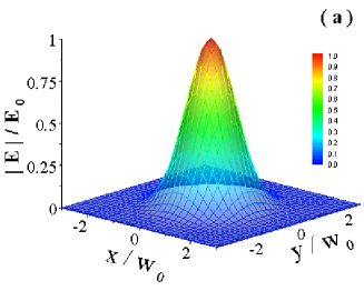
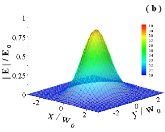
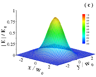
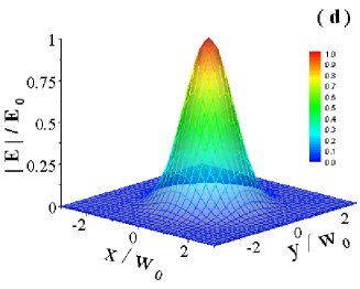
Figure 5: (Color online) The numerically computed intensity distribution in object and image planes. (a) the intensity distribution for normal Gaussian beam in object plane. The in tensity distribution in image plane for Gaussian beam propagating through the QIMM slab with different anisotropic parameters: (b) $n_{x}=-1$, $n_{y}=-2$. (c) $n_{x}=-2$, $n_{y}=-1$. (d) $n_{x}=-1$, $n_{y}=-1$. We can easily find the intensity distribution at the object plane can be completely reconstructed at the image plane.

Finally we want to explore the field in region $3$. The field in the second boundary can be easily obtained from Eq. (40) under choosing $z=a+d$. Substituting the field into Eq. (29), the angular spectrum distribution can be written as

$$\tilde{\bf E}_{3}({\bf k}_{\perp})=\frac{w_{0}E_{0}}{\sqrt{2\pi}}\exp\left[-\left(\frac{n_{x}k_{0}w_{0}^{2}+2in_{x}a+2id}{4n_{x}k_{0}}k_{x}^{2}+\frac{n_{y}k_{0}w_{0}^{2}+2in_{y}a+2id}{4n_{y}k_{0}}k_{y}^{2}\right)\right].$$ (42)

Substituting Eq. (42) into Eq. (27), the field in the region 3 is given by

$${\bf E}_{3}({\bf r}_{\perp},z_{3}^{\ast})=\frac{w_{0}E_{0}}{\sqrt{w_{3x}w_{3y}}}\exp\left[-\left(\frac{x^{2}}{w_{3x}^{2}}+\frac{y^{2}}{w_{3y}^{2}}\right)+i\psi_{3}\right],$$ (43)

$$w_{3x}=w_{0}\sqrt{1+\left(\frac{z_{3x}^{\ast}}{L_{3x}}\right)^{2}},~{}~{}~{}w_{3y}=w_{0}\sqrt{1+\left(\frac{z_{3y}^{\ast}}{L_{3y}}\right)^{2}}.$$ (44)

Here $z_{3x}^{\ast}=z-(1-1/n_{x})d$ and $z_{3y}^{\ast}=z-(1-1/n_{y})d$. The corresponding Rayleigh lengths give by $L_{3x}=L_{3y}=k_{0}w_{0}^{2}/2$, that denote the beam exhibit the same diffraction distance in the direction of $x$ and $y$ axes. The effect of the anisotropic diffraction is that these two beam widths keep their difference even if the Rayleigh lengths, $L_{3x}$ and $L_{3y}$, are equal, implying that generally the Gaussian beam is astigmatic.

Up to now, the fields are determined explicitly in the three regions. Comparison of Eq. (40), Eq. (43) with Eq. (37) shows that the field distributions in region $2$ and region $3$ may no longer remain Gaussian. We take the image position $z=a+d+b$ to be the place of the second focusing waist. For the purpose of illustration, the intensity distribution in object plane is plotted in Fig. 5(a). In general, the shape of intensity distribution is distorted in image plane as shown in Fig. 5(b) and Fig. 5(c). Careful evaluation of Eq. (43) reveals that the secret underlying the intensity distortion is the anisotropic diffraction.

Now, the most obvious question is whether the intensity distribution at the object plane can be completely reconstructed at the image plane. In the next step, we want to explore the matching condition of focusing. We can easily obtain the place of the focusing waist by choosing $z^{\ast}_{i}=0$. Let us assume the incident beam waist locates at plane $z=0$. To eliminate the astigmatic effect, the beam waists should locate at the same place, namely $z_{3x}^{\ast}=z_{3y}^{\ast}$. Using these criterions, the matching condition for focusing can be written as

$$\varepsilon_{y}\mu_{z}(a+b)+\sigma\sqrt{\varepsilon_{x}\mu_{y}}d=0,~{}~{}~{}\varepsilon_{x}=\varepsilon_{y}.$$ (45)

Under the focusing matching condition, the intensity distribution at the object plane can be completely reconstructed at the image plane as shown in Fig. 5(d). A further point should be noted is that the thickness of the QIMM slab should satisfy the relation $d>\sigma\varepsilon_{y}\mu_{z}a/\sqrt{\varepsilon_{x}\mu_{y}}$, otherwise there is neither an internal nor an external focus.

V Phase compensation by polarization insensitive lens

In this section, we attempt to investigate the matching condition for phase compensation. In isotropic LHM, plane waves can propagate with negative phase velocity directed opposite to the direction of Poynting vector. Hence the phase difference can be compensated by the LHM slab Veselago1968 ; Pendry2000 ; Luo2006b . However, the negative tensor parameters associated with QIMM provides a wealth of opportunities for observing and exploiting negative phase-velocity behavior.

First let us investigate the phase distribution in region 1. A more rigorous calculation of Eq. (37) gives

$$\psi_{1} = k_{0}z+\left(\frac{k_{0}x^{2}}{2R_{1x}}+\frac{k_{0}y^{2}}{2R_{1y}}\right)-\Phi_{1},$$ (46)

$$R_{1x} = z_{1x}^{\ast}+\frac{L_{1x}^{2}}{z_{1x}^{\ast}},~{}~{}~{}R_{1y}=z_{1y}^{\ast}+\frac{L_{1y}^{2}}{z_{1y}^{\ast}},$$ (47)

$$\Phi_{1} = -\frac{1}{2}\left(\arctan\frac{z_{1x}^{\ast}}{L_{1x}}+\arctan\frac{z_{1y}^{\ast}}{L_{1y}}\right).$$ (48)

Here $R_{1x}$ and $R_{1y}$ are the radius of curvature. Because of the isotropy in vacuum, we can easily find $R(z_{1x}^{\ast})=R(z_{1y}^{\ast})$. The Gouy phase shift in vacuum is given by $\Phi_{1}$.

Next, we attempt to explore the phase distribution in region 2. Matching the boundary condition, the phase term in Eq. (40) can be written as

$$\psi_{2} = k_{0}a+\sigma\sqrt{\varepsilon_{y}\mu_{x}}k_{0}(z-a)+\frac{k_{0}x^{2}}{2R_{2x}}+\frac{k_{0}y^{2}}{2R_{2y}}-\Phi_{2},$$ (49)

$$R_{2x} = z_{2x}^{\ast}+\frac{L_{2x}^{2}}{z_{2x}^{\ast}},~{}~{}~{}R_{2y}=z_{2y}^{\ast}+\frac{L_{2y}^{2}}{z_{2y}^{\ast}},$$ (50)

$$\Phi_{2} = -\frac{1}{2}\left(\arctan\frac{z_{2x}^{\ast}}{L_{2x}}+\arctan\frac{z_{2y}^{\ast}}{L_{2y}}\right).$$ (51)

The Gouy phase shift in QIMM is given by Eq. (51). We should mention that there are two different radius of curvature, $R_{2x}$ and $R_{2y}$, that characterize the beam undergo different diffraction effects in the direction of $x$ and $y$ axes, respectively.

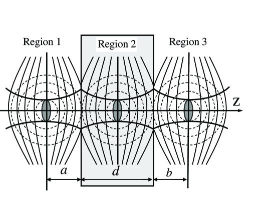
Figure 6: The phase difference caused by the Gouy phase shift in vacuum can be compensated by that caused by the inverse Gouy phase shift in the QIMM slab. The phase fronts of Gaussian beam (solid lines) differ from those of a perfect spherical wave (dashed lines).

Now, we are in the position to explore the phase distribution in region 3. Analogously, we make some serious calculation of Eq. (43), then obtain the phase distribution

$$\psi_{3} = \sigma\sqrt{\varepsilon_{y}\mu_{x}}k_{0}d+k_{0}(z-d)+\frac{k_{0}x^{2}}{2R_{3x}}+\frac{k_{0}y^{2}}{2R_{3y}}-\Phi_{3},$$ (52)

$$R_{3x} = z_{3x}^{\ast}+\frac{L_{3x}^{2}}{z_{3x}^{\ast}},~{}~{}~{}R_{3y}=z_{3y}^{\ast}+\frac{L_{3y}^{2}}{z_{3y}^{\ast}},$$ (53)

$$\Phi_{3} = -\frac{1}{2}\left(\arctan\frac{z_{3x}^{\ast}}{L_{3x}}+\arctan\frac{z_{3y}^{\ast}}{L_{3y}}\right).$$ (54)

The radius of curvatures are given by Eq. (53) and the corresponding Gouy phase shift is given by Eq. (54). The anisotropic effect result in the two radius of curvatures keep their difference even if the Rayleigh lengths are equal.

It is known that an electromagnetic beam propagating through a focus experiences an additional $\pi$ phase shift with respect to a plane wave. This phase anomaly was discovered by Gouy in 1890 and has since been referred to as the Gouy phase shift Born1997 ; Feng2001 . It should be mentioned that there exists an effect of accumulated Gouy phase shift when a beam passing through an optical system with positive index Erden1997 ; Feng1999 ; Feng2000 . While in the QIMM slab system we expect that the phase difference caused by Gouy phase shift can be compensated by that caused by the inverse Gouy shift in the QIMM slab.

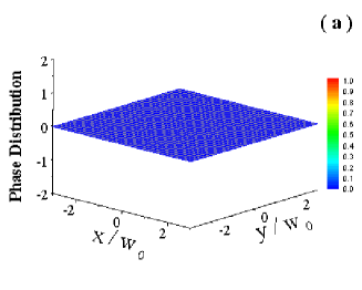
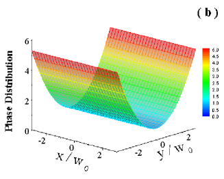
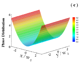
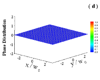
Figure 7: (Color online) The numerically computed phase distribution in object and image planes. (a) The phase distribution in object plane. The phase distribution in image plane after the Gaussian beam propagating through the QIMM slab with different anisotropic parameters: (b) $n_{x}=-1$, $n_{y}=-2$. (c) $n_{x}=-2$, $n_{y}=-1$. (d) $n_{x}=-1$, $n_{y}=-1$. The phase distribution can be completely reconstructed at the image plane. The parameters are the same as in Fig. 5.

We might suspect whether the phase difference caused by the Gouy phase shift in vacuum can be compensated by that caused by the inverse Gouy phase shift in QIMM slab. To obtain the better physical picture, the schematic distribution of phase fronts are plotted in Fig. 6. The phase fronts of a focused Gaussian beam are plotted with solid lines, and the phase fronts of a perfect spherical wave are depicted with the dashed lines. The phase difference on the optical axis is caused by the Gouy phase shift. The inherent secret underlying the reverse Gouy phase shift in the QIMM slab is the waves undergo a negative phase velocity.

Let us investigate what happens if we consider the phase difference caused by the Gouy shift. Under the focusing matching conditions, the phase difference caused by the Gouy phase shift in the three regions are

$$\Delta\Phi_{1} = -\arctan\frac{a}{z_{R}},$$

$$\Delta\Phi_{2} = \arctan\frac{a}{z_{R}}+\arctan\frac{b}{z_{R}},$$

$$\Delta\Phi_{3} = -\arctan\frac{b}{z_{R}}.$$ (55)

The first and third equations dictate the phase difference caused by the Gouy shift in regions $1$ and $3$, respectively. The second equation denotes the phase difference caused by the inverse Gouy phase shift in the QIMM slab. Subsequent calculations of Eq. (55) show

$$\Delta\Phi_{1}+\Delta\Phi_{2}+\Delta\Phi_{3}=0.$$ (56)

This implies that the phase difference caused by the Gouy phase shift in vacuum can be compensated by the counterpart caused by the inverse Gouy phase shift in QIMM slab. Therefore the condition for phase compensation can be simply written as

$$(a+b)k_{0}+\sigma\sqrt{\varepsilon_{y}\mu_{x}}dk_{0}=0.$$ (57)

The first term in Eq. (57) is the phase deference caused by the plane wave in vacuum, and the other term is the phase deference caused by the plane wave in the QIMM slab.

For the purpose of illustration, the phase distribution in object plane is plotted in Fig. 7(a). Generally, the phase distributions in image plane is distorted as shown in Fig. 7(b) and Fig. 7(c). As mentioned above, the phase distortion is caused by the effect of anisotropic diffraction. To cancel the phase distortion, the beam waists should locate at the same place, namely $z_{3x}^{\ast}=z_{3y}^{\ast}$. Under the phase matching condition, the phase distribution at the object plane can also be completely reconstructed at the image plane as depicted in Fig. 7(d).

Now an interesting question naturally arises: whether the matching conditions of focusing and the phase compensation can be satisfied simultaneously. Clearly, if we seek a solution satisfying Eqs. (45) and (57), the only possibility is

$$\varepsilon_{x}=\varepsilon_{y},~{}~{}~{}\varepsilon_{y}\mu_{z}=1.$$ (58)

Under the matching conditions, the intensity and phase distributions at the object plane can be completely reconstructed at the image plane.

It should be mentioned that, for the QIMM slab with double-sheeted hyperboloid wave-vector surface, both E- and H-polarized beams can also exhibit the same intensity and phase reconstructed effect. Because of the positive phase velocity embedded in this type of QIMM, the paraxial beam will experience the positive Rayleigh distance and Gouy phase shift. Therefore the accumulated phase delay effect give rise to a large phase deference between the object and image planes.

VI The transmission of evanescent waves

In this section, we discuss under what conditions anomalous transmission will occur when an evanescent wave transmitted through the QIMM slab. It is well known that when an evanescent wave is transmitted through a slab of regular media with simultaneously positive permittivity and permeability, the amplitude of the transmitted wave will decay exponentially as the thickness of the slab increases. While an evanescent wave transmitted through an isotropic LHM slab, the amplitude of the transmitted wave would be amplified exponentially. This anomalous transmission of evanescent waves is a very peculiar property of LHM and it may lead to subwavelength image Pendry2000 ; Fang2005 .

Now we will explore what happen when the evanescent wave transmission through the QIMM slab. For E-polarized incident waves, the incident and reflected fields in region 1 can be written as

$${\bf E}_{1}=E_{0}{\bf e}_{y}\exp[i(k_{x}x+k_{z}z)]+R_{E}E_{0}{\bf e}_{y}\exp[i(k_{x}x-k_{z}z)],$$ (59)

where $R_{E}$ is the reflection coefficient. Some of the incident wave is transmitted into the QIMM slab, and conversely a wave inside the QIMM slab incident on its interfaces with the surrounding vacuum also experiences transmission and reflection, so the electric field of the wave inside the slab is given by

$${\bf E}_{2}=rE_{0}{\bf e}_{y}\exp[i(q_{x}^{E}x+q_{z}^{E}z)]+tE_{0}{\bf e}_{y}\exp[i(q_{x}^{E}x-q_{z}^{E}z)].$$ (60)

Here $r$ and $t$ are coefficients which need to be determined by boundary conditions Hu2002 . Matching the boundary conditions for each wave-vector component at the plane $z=a+d$ gives the propagation field in the form

$${\bf E}_{3}=T_{E}E_{0}{\bf e}_{y}\exp[iq_{x}^{E}x+q_{z}^{E}(z-d)],$$ (61)

where $T_{E}$ is the overall transmission coefficient. The $z$-component of the wave vectors of evanescent waves can be found by the solution of Eq. (12), which yields

$${q_{z}^{E}}=i\sqrt{\frac{\mu_{x}}{\mu_{z}}q_{x}^{2}-\varepsilon_{y}\mu_{x}k_{0}^{2}},~{}~{}~{}{q_{z}^{H}}=i\sqrt{\frac{\varepsilon_{x}}{\varepsilon_{z}}q_{x}^{2}-\varepsilon_{x}\mu_{y}k_{0}^{2}},$$ (62)

for E- and H-polarized waves, respectively.

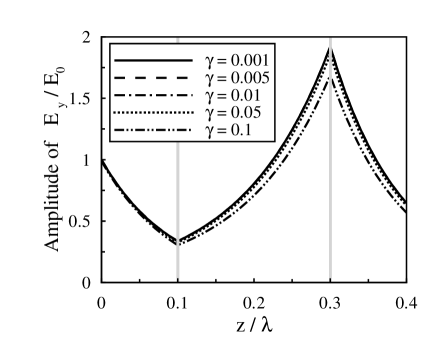
Figure 8: An evanescent wave ($k_{x}=2k_{0}$) interacting with a QIMM slab (a) $d=0.2\lambda$ (b) $d=0.4\lambda$. The QIMM with different values of absorption $\gamma_{e}=\gamma_{m}=\gamma$, ranging from 0.001 to 0.1. The QIMM slab is supposed to be well satisfied the conditions: $\varepsilon_{x}=\varepsilon_{y}=-0.8-\gamma i$ and $\mu_{z}=-1.25-\gamma i$. The vertical gray lines denote the two surfaces of the QIMM slab.

By matching the electric and magnetic fields at the two interfaces between the QIMM slab and the surrounding vacuum, the coefficients in Eqs. (59), (60), and (61) can be determined. We can get that the overall transmission through both surfaces of the QIMM slab is given by

$$T_{E}=\frac{4\mu_{x}k_{z}q_{z}^{E}\exp(iq_{z}^{E}d)}{(\mu_{x}k_{z}+q_{z}^{E})^{2}-(q_{z}^{E}-\mu_{x}k_{z})^{2}\exp(2iq_{z}^{E}d)},$$ (63)

From Eq. (63) we can see that in general cases, when an evanescent wave is transmitted through a QIMM slab, its amplitude will decay exponentially as the thickness of the slab increases. But if the following conditions are satisfied:

$$\mu_{x}<0,~{}~{}\mu_{z}<0,~{}~{}\varepsilon_{y}<0,$$ (64)

$$\varepsilon_{x}\mu_{z}=1,~{}~{}~{}\varepsilon_{y}\mu_{z}=1,$$ (65)

the amplitude of the transmitted evanescent wave will be amplified exponentially by the transmission process through the QIMM slab. From Eq. (63), we can see that if the conditions (64) and (65) are satisfied, the overall transmission coefficient $T_{E}$ will be equal to $\exp(|q_{z}^{E}|d)$, hence the amplitude of the transmitted evanescent wave will be amplified exponentially as the thickness of the QIMM slab increases. Note that the conditions mentioned above are sightly different from those as Hu and Chui have obtained Hu2002 .

As for H-polarized evanescent waves, the overall transmission through both interfaces of the QIMM slab can be obtained by similar procedures, and we can get the overall transmission coefficient:

$$T_{H}=\frac{4\varepsilon_{x}k_{z}q_{z}^{H}\exp(iq_{z}^{H}d)}{(\varepsilon_{x}k_{z}+q_{z}^{H})^{2}-(q_{z}^{H}-\varepsilon_{x}k_{z})^{2}\exp(2iq_{z}^{H}d)}.$$ (66)

From Eq. (66), we can see that in general cases, the amplitude of the transmitted H-polarized evanescent waves will also decay exponentially as the thickness of the QIMM slab increases. But if the following conditions are satisfied, the overall transmission coefficient $T_{H}$ will be equal to $\exp(|q_{z}^{H}|d)$, and the amplitude of the transmitted H-polarized evanescent wave will be amplified exponentially by the transmission process through the QIMM slab. So for H-polarized evanescent waves,

$$\varepsilon_{x}<0,~{}~{}\varepsilon_{z}<0,~{}~{}\varepsilon_{y}<0,$$ (67)

$$\varepsilon_{z}\mu_{x}=1,~{}~{}~{}\varepsilon_{z}\mu_{y}=1.$$ (68)

if conditions (67) and (68) are satisfied, the QIMM slab will enhance exponentially the transmitted waves. Comparing (64) and (65) with (67) and (68), we find that in the presence of QIMM, the conditions for E-polarized means automatically the conditions for H-polarized are satisfied. Hence the QIMM also exhibit the significant insensitive effect for evanescent waves. We stress that, for the QIMM slab with double-sheeted hyperboloid dispersion relation, the evanescent waves cannot be amplified.

In the above analysis the permittivity and permeability tensor elements are assumed to be lossless. However the effect of absorption, necessarily present in such materials, may drastically suppress any evanescent amplifying wave into a decaying one Garcia2002 ; Rao2003 . Comparing Fig. 8(a) with Fig. 8(b) suggests that large $d$ is not favored for the amplification of the evanescent wave inside the QIMM slab. It is also clearly seen from Figs. 8(a) and 8(b) that a low reflection occurs at the interfaces, since the QIMM slab is supposed to be well satisfied the conditions (64) and (65). So far we have shown the simulation results of the evanescent wave interacting with QIMM slabs with different absorptions and thicknesses. We find that the suppression of evanescent-wave amplification can be effectively relaxed by reducing the thickness of the QIMM slab. The numerical examples provide direct evidence that an evanescent wave could be amplified in a QIMM slab with finite absorption. Unfortunately, the loss of a realistic metamaterial could not be reduced to a very small level Shen2003 . Therefore, the thickness of the QIMM slab should be much smaller than the wavelength in order to realize the subwavelength imaging for such a system.

As a result of the amplification of evanescent waves inside the lossy QIMM slab, superlensing effect with subwavelength image resolution could be achieved practically. While the main effect of anisotropy associated with QIMM will limit the resolution of the image. Although the image is imperfect, we trust that the reconstruct effect of intensity and phase in paraxial regime will lead to some potential applications. Several recent developments make the polarization insensitive lens a practical possibility. Some time ago it was shown that a double-periodic array of pairs of parallel gold nanorods will exhibit negative permittivity and permeability in the optical range Shalaev2005 ; Kildishev2006 . Another extremely promising material has been previously explored in certain designs of photonic crystals, which can be effectively modelled with anisotropic permittivity and permeability tensors Shvets2003 ; Shvets2004 ; Urzhumov2005 . Experimentally, the goal to realize the insensitive lens, chiefly lies in reducing the loss of QIMM. Practical polarization insensitive lens will require the frequency independent, a great challenge to the designers is to realize the negative material parameters in a wide band. The recent developments lead us to be optimistic that the polarization insensitive lens can be designed in future.

VII Conclusions

In conclusion, we have proposed how to employ the QIMM slab to create a polarization insensitive lens, in which both E- and H-polarized waves exhibit the same refocusing effect. For shallow incident angles the QIMM slab will provide some degree of refocusing in the same manner as an isotropic negative index material. We have investigated the focusing and phase compensation of paraxial beams by the QIMM slab. We have introduced the concepts of inverse Gouy phase shift and negative Rayleigh length of paraxial beams in QIMM. We have shown that the phase difference caused by the Gouy phase shift in vacuum can be compensated by that caused by the inverse Gouy phase shift in the QIMM slab. If certain matching conditions are satisfied, the intensity and phase distributions at object plane can be completely reconstructed at the image plane. The QIMM slab exhibits the significant insensitive effect for both transmitted and evanescent waves. Our simulation results show that the superlensing effect with subwavelength image resolution could be achieved in the form of a QIMM slab. We wish the essential physics described in this paper will provide reference in the road to construct the polarization insensitive lens. We trust that the significant insensitive properties will lead to further novel effects and applications.

- (1) V. G. Veselago, Sov. Phys. Usp. 10, 509 (1968).
- (2) D. R. Smith, W. J. Padilla, D. C. Vier, S. C. Nemat-Nasser, and S. Schultz, Phys. Rev. Lett. 84, 4184 (2000).
- (3) R. A. Shelby, D. R. Smith, and S. Schultz, Science 292, 77 (2001).
- (4) J. Pacheco Jr., T. M. Grzegorczyk, B. I. Wu, Y. Zhang, J. A. Kong, Phys. Rev. Lett. 89, 257401 (2002).
- (5) C. G. Parazzoli, R. G. Greegpr, K. Li, B. E. C. Koltenba, and M. Tanielian, Phys. Rev. Lett. 90, 107401 (2003).
- (6) A. A. Houck, J. B. Brock, and I. L. Chuang, Phys. Rev. Lett. 90, 137401 (2003).
- (7) M. Notomi, Phys. Rev. B 62, 10696 (2000).
- (8) C. Luo, S. G. Johnson, J. D. Joannopoulos, and J. B. Pendry, Phys. Rev. B 65, 201104(R) (2002).
- (9) C. Luo, S.G. Johnson, and J. D. Joannopoulos, Appl. Phys. Lett. 81, 2352 (2002).
- (10) J. Li, L. Zhou, C. T. Chan, and P. Sheng, Phys. Rev. Lett. 90, 083901 (2003).
- (11) I. V. Lindell, S. A. Tretyakov, K. I. Nikoskinen, and S. Ilvonen, Microw. Opt. Technol. Lett. 31, 129 (2001).
- (12) L. Hu and S. T. Chui, Phys. Rev. B 66, 085108 (2002).
- (13) D. R. Smith and D. Schurig, Phys. Rev. Lett. 90, 077405 (2003).
- (14) Y. Zhang, B. Fluegel and A. Mascarenhas, Phys. Rev. Lett. 91, 157404 (2003).
- (15) L. Zhou, C. T. Chan, and P. Sheng, Phys. Rev. B 68 115424 (2003).
- (16) H. Luo, W. Hu, X. Yi, H. Liu and J. Zhu, Opt. Commun. 254, 353 (2005).
- (17) Z. M. Thomas, T. M. Grzegorczyk, B. I. Wu, X. Chen, and J. A. Kong, Opt. Express, 13, 4737 (2005).
- (18) H. Luo, W. Hu, W. Shu, F. Li and Z. Ren, Europhysics Letters, 74, 1081 (2006).
- (19) T. M. Grzegorczyk and J. A. Kong, Phys. Rev. B 74, 033102 (2006).
- (20) J. B. Pendry, Phys. Rev. Lett. 85, 3966 (2000).
- (21) D. R. Smith, D. Schurig, J. J. Mock, P. Kolinko, and P. Rye, Appl. Phys. Lett. 84, 2244 (2004).
- (22) D. R. Smith, P. Kolinkp, and D. Schurig, J. Opt. Soc. Am. B 21, 1032 (2004).
- (23) C. G. Parazzoli, R. B. Greegor, J. A. Nielsen, M. A. Thompson, K. Li, A. M. Vetter, and D. C. Vier, Appl. Phys. Lett. 84, 3232 (2004).
- (24) T. Dumelow, J. A. P. da Costa, and V. N. Freire, Phys. Rev. B 72, 235115 (2005).
- (25) H. C. Chen, Theory of Electromagnetic Waves (McGraw-Hill, New York, 1983).
- (26) N. H. Shen, Q. Wang, J. Chen, Y. X. Fan, J. Ding, H. T. Wang, Y. Tian, and N. B. Ming, Phys. Rev. B 72, 1531041 (2005).
- (27) H. Luo, W. Shu, F. Li, and Z. Ren, Opt. Commun. 266, 327 (2006).
- (28) J. W. Goodman, Introduction to Fourier Optics (McGraw-Hill, New York, 1996).
- (29) M. Lax, W. H. Louisell and W. McKnight, Phys. Rev. A 11, 1365 (1975).
- (30) A. Ciattoni, B. Crosignani, and P. Di Porto, Opt. Commun. 177, 9 (2000).
- (31) H. Luo, W. Hu, Z. Ren, W. Shu, and F. Li, Opt. Commun. 267, 271 (2006).
- (32) M. Born and E. Wolf, Principles of Optics (University Press, Cambridge, 1997 ).
- (33) S. Feng and H. G. Winful, Opt. Lett. 26, 485 (2001).
- (34) M. F. Erden and H. M. Ozaktas, J. Opt. Soc. Am. A 14, 2190 (1997).
- (35) S. Feng and H. G. Winful, J. Opt. Soc. Am. A 16, 2500 (1999).
- (36) S. Feng and H. G. Winful, Phys. Rev. E 61, 862 (2000).
- (37) N. Fang, H. Lee, C. Sun, and X. Zhang, Science 308, 534 (2005).
- (38) N. Garcia and M. Nieto-Vesperinas, Phys. Rev. Lett. 88, 207403 (2002).
- (39) X. S. Rao and C. K. Ong, Phys. Rev. B 88, 113103 (2003).
- (40) L. Shen and S. He, Phys. Lett. A 309, 298 (2000).
- (41) V. M. Shalaev, W. Cai, U. K. Chettiar, Hsiao-Kuan Yuan, A. K. Sarychev, V. P. Drachev, and A. V. Kildishev, Opt. Lett. 30, 3356 (2005).
- (42) A. V. Kildishev, W. Cai, U. K. Chettiar, Hsiao-Kuan Yuan, A. K. Sarychev, V. P. Drachev, and V. M. Shalaev, J. Opt. Soc. Am. B 23, 423 (2006).
- (43) G. Shvets, Phys. Rev. B 67, 0351091 (2003).
- (44) G. Shvets and Y. A. Urzhumov, Phys. Rev. Lett. 93, 2439021 (2004).
- (45) Y. A. Urzhumov and G. Shvets, Phys. Rev. E 72, 026608 (2005).