An efficient algorithm simulating a macroscopic system at the critical point

Abstract

It is well known that conventional simulation algorithms are inefficient for the statistical description of macroscopic systems exactly at the critical point due to the divergence of the corresponding relaxation time (critical slowing down). On the other hand the dynamics in the order parameter space is simplified significantly in this case due to the onset of self-similarity in the associated fluctuation patterns. As a consequence the effective action at the critical point obtains a very simple form. In the present work we show that this simplified action can be used in order to simulate efficiently the statistical properties of a macroscopic system exactly at the critical point. Using the proposed algorithm we generate an ensemble of configurations resembling the characteristic fractal geometry of the critical system related to the self-similar order parameter fluctuations. As an example we simulate the one-component real scalar field theory at the transition point $T=T_{c}$ as a representative system belonging to the $3-D$ Ising universality class.

I Introduction

The traditional simulation algorithms of statistical mechanics are proven to be inefficient for the simulation of the statistical properties of macroscopic systems at a critical point. This is a consequence of the well-known mechanism of critical slowing down leading to a divergence of the relaxation time, independently of the algorithm used, when the critical point is reached Barkema99 . Therefore, the generation of an ensemble of configurations carrying the properties of the critical system is in practice a very difficult task as the onset of equilibrium is prerequisite. On the other hand, due to the universal character of the correlations at the critical point, the dynamics of the order parameter, described effectively through the averaged action Wetter93 or the constrained effective potential Kyriak , acquire a very simple form Tetrad02 ; Tsypin94 reflecting the self-similarity of the associated fluctuation pattern. The consequence of self-similarity at the macroscopic level is at best reflected in the fractal geometry of the domains with constant magnetization in an Ising ferromagnet. However, fractality in the strict mathematical sense is only defined for an ideal critical system embedded in a continuous space. In real physical systems fractal geometry occurs only partially between some well defined scales. Therefore, physical fractals, contrary to the corresponding exact mathematical sets, can be defined also on equidistant lattices facilitating their realization through numerical simulations. On the other hand, a realistic algorithm generating critical configurations of a system at its transition point should also reproduce the (partial) fractal geometry of the critical clusters. There are several ways to produce sets with prescribed fractal dimension found in the literature Mandel83 . The associated algorithms can either be of stochastic Alemany94 or deterministic nature Cantor . However, although fractal geometry is strongly related to critical phenomena, there is, up to now, no algorithm capable to link directly this geometrical property with the statistical mechanics of a critical system.

The present work attempts a step in this direction. The main goal is to develop an efficient algorithm for the simulation of a macroscopic system at the critical point. In fact we propose a method able to generate an ensemble of microstates of the considered system carrying its basic critical properties such as self-similar order parameter fluctuations and algebraically decaying spatial correlations Stanley . Using the representation of the partition function in terms of the effective free energy at the critical point we proceed within the saddle point approximation. Then we show that the associated functional measure can be expressed as a summation over piecewise constant configurations of the order parameter within domains (clusters) of variable size covering the entire critical system. We use these configurations to calculate the ensemble averaged density-density correlation function leading to a power-law form characteristic of a fractal set. Thus we recover a relation between the fractal geometry of the critical clusters and the canonical ensemble of critical configurations describing the statistical properties of the system at the transition point.

The generation of an ensemble of critical configurations is of relevance for the study of the evolution of a critical system under the influence of an external potential removing it from the initial critical state. In this case the determined critical ensemble is introduced as a set of initial conditions for the corresponding dynamical problem manosarchive . Besides, one can also consider the time evolution of a critical system under the constraints of thermodynamical equilibrium so that the property of self-similarity sustains for an infinitely long time interval. This situation could be actually realized in the case of biological systems for which there exist several indications that they are permanently on a critical state Chialvo06 .

The paper is organized as follows: in section II we describe the basic ingredients of the proposed algorithm for the construction of a random fractal measure on a lattice. In section III, subsection (A), we study in detail the one dimensional case. For a genuine $1-D$ system with short range interactions, critical behavior is not possible Peierls . However, it turns out that the $1-D$ version of the algorithm is optimal for the illustration of the basic steps of the procedure. In addition, an $1-D$ effective theory describing the projection of a $3-D$ critical system, can in principle carry imprints of the critical state. In subsection (III B), we extend the proposed algorithm for the general $D-$dimensional case. Finally, in section IV we summarize our concluding remarks.

II Saddle point approach for single cluster $\varphi$-configurations at the critical point

There are two extreme situations where the division of the whole system to subsystems and the subsequent study of one of them, is a good approximation. The first is when the interactions are very weak so that statistical independence is valid, and the whole system can be assumed to be constituted by separated building blocks. On the opposite limit, in a critical system, where the correlations are very strong, we expect the emergence of self-similarity and the formation of fractal structures. In this case investigation of a small region offers information for the entire system. Thus, at the critical point, it is natural to consider the partition function $Z_{\Omega}$ of an open subdomain $\Omega$ of a critical cluster. Assuming that the order parameter is an one-component real field $\varphi$, $Z_{\Omega}$ is given as:

$$Z_{\Omega}=\int{\cal{\delta}}[\varphi]e^{-\Gamma[\varphi,\Omega]},$$ (1)

in terms of the effective action:

$$\Gamma[\varphi,\Omega]=\int_{\Omega}d^{D}x\{\frac{1}{2}(\nabla\varphi(\vec{x}))^{2}+g\varphi^{\delta+1}(\vec{x})\},$$ (2)

expected to be valid at the critical point $T=T_{c}$ Tetrad02 ; Tsypin94 . In (2) $\delta$ is the isothermal critical exponent Stanley . To calculate the partition function (1) one may use the saddle point approach developed in Anton98 where it is shown that the functional sum in $Z_{\Omega}$ is saturated by the summation over the saddle point solutions of the effective action (2). These solutions encompass power-law singularities. In the sum (1) the only significant contribution comes from those saddle points for which the corresponding singularities lie outside the region $\Omega$. In fact, if the distance of the location of the singularities from the boundary of the domain $\Omega$ increases, the corresponding statistical weight increases too. In this case the saddle point solutions can be well approximated by constant functions inside $\Omega$ Anton98 .

Since in the present work we are mainly interested in the calculation of the density-density correlation function, it is necessary to extend the saddle point method to the case of the generalized effective action:

$$\Gamma_{G}[\varphi,\Omega]=\int_{\Omega}d^{D}x\{\frac{1}{2}(\nabla\varphi(\vec{x}))^{2}+g\varphi^{\delta+1}(\vec{x})+j\varphi(\vec{x})\delta(\vec{x})\},$$ (3)

involving a source term at $\vec{x}=0$. The saddle point solutions of (3) obey the evolution equation:

$$\nabla^{2}\varphi(\vec{x})-g(\delta+1)|\varphi(\vec{x})|^{\delta}=j\delta({\vec{x}}).$$ (4)

Interpreting $|\varphi(\vec{x})|$ as density the associated ensemble of saddle point solutions is statistically identical to the density-density correlation function $\langle|\varphi(\vec{x})\varphi(\vec{0})|\rangle$, in the limit $j\rightarrow 0$ huang . Note that the presence of the source at $\vec{x}=0$ does not affect the generality and we can use any other point as reference.

In order to simplify the presentation of the generalized saddle point calculation, in the following we will describe the one-dimensional case. However, as mentioned above, critical behavior, in the absence of long range interactions, occurs only in higher dimensional systems. Thus, the $1-D$ case should be considered as a valuable explanatory tool allowing also for analytical results, or as an effective description of the $1-D$ projection of a higher dimensional critical system. In analogy with the treatment in Anton98 , eq.(4) is solved as an initial value problem. The solution in one dimension is given implicitly in terms of the function:

$$H(\varphi,E)=\frac{2}{(\delta+1)}g^{-\frac{1}{\delta+1}}\sqrt{E+g|\varphi|^{\delta+1}}E^{-\frac{\delta}{\delta+1}}\,F\left(\frac{1}{2},\frac{\delta}{\delta+1},\frac{3}{2},1+\frac{g|\varphi|^{\delta+1}}{E}\right),$$ (5)

where $E$ is a parameter depending on the assumed initial conditions and having the interpretation of the total energy of the system. $F\left(\alpha,\beta;\gamma;z\right)$ is the usual hypergeometric function RZ . For $x\geq 0$ the saddle point solutions are the inverse function of:

$$x=H(\varphi(x),E_{+})-H(\varphi(0),E_{+}),$$ (6)

while for $x<0$ they are the inverse function of

$$x=H(\varphi(x),E_{-})-H(\varphi(0),E_{-}).$$ (7)

Due to the source term the energy of the system varies in the two half-spaces and the corresponding energy difference is determined by the formula:

$$E_{-}=E_{+}+\frac{j^{2}}{2}+j\sqrt{2\left(E_{+}+g|\varphi(0)|^{\delta+1}\right)},$$ (8)

In the limit $j\rightarrow 0$, $E_{-}=E_{+}=E$ and these solutions simplify to those presented in Anton98 .

Similarly to the previous discussion, a typical generalized saddle point solution possesses two singularities which can be seen in the graphical presentation in fig 1.

Figure 1: A typical generalized saddle point solution, obtained analytically, for the $1-D$ case. The discontinuity of the derivative at $x=0$ is clearly seen in the inset figure.

Additionally it possesses a discontinuity in the field derivative at $x=0$ which vanishes in the limit $j\rightarrow 0$. In analogy to the case without the source term, the summation over the generalized saddle points is also dominated by configurations for which the singularities lie beyond the range of the cluster. Therefore, the solutions (6),(7) which contribute significantly to the system’s partition function can also be well approximated by a constant function within the cluster.

The saddle point solutions in the higher dimensional case are impossible to be found analytically. However numerical calculations reveal a similar behavior, that is almost constant configurations with singularities forming a closed $D-1$ subspace around the location of the source, which can be handled as described above. Therefore, the summation over the saddle point solutions in the single cluster partition function, in any space dimension $D$, can be well approximated by an ordinary integration over constant field configurations.

The fractal geometry of the critical clusters is revealed through the power-law dependence of the density-density correlation function which in turn leads to a power-law dependence of the mean “mass” $m(R)$ within a domain of radius $R$ around $\vec{x}_{0}=\vec{0}$:

$$m(R)\sim R^{D_{f}},$$ (9)

with the exponent $D_{f}$ in (9) being the so-called fractal mass dimension Mandel83 ; Vicsek ; Falconer . Alternatively, using the saddle-point ensemble defined above the mean “mass” can be calculated as:

$$m(R)=\langle\int_{R}|\varphi(\vec{x})\varphi(\vec{0})|\,d^{D}x\rangle.$$ (10)

For a critical system at thermal equilibrium $D_{f}$ is related to the critical exponent $\delta$, appearing in the effective action (2), as well as the dimension $D$ of the embedding space through stinchcombe :

$$D_{f}=\frac{D\delta}{\delta+1}.$$ (11)

The analysis at the level of one cluster is not sufficient for the description of the properties of the entire critical system. Therefore, after obtaining the set of saddle-point solutions of the generalized action (3), it is necessary to use it in order to generate an ensemble of configurations valid for the global system. The systematic way to perform this extension is explained in detail in the next section.

III Generation of multi-cluster configurations for the critical system

In order to generate an ensemble of global configurations for the critical system within the saddle point approach discussed in the previous section one adopts the following picture: The entire system is composed of weakly correlated clusters of different size up to the correlation length Anton98 (which at the critical point is expected to be of the order of the lattice size). Thus, for given number and size of clusters, the partition function of the system can be decomposed in the product of the partition functions of each cluster. The sum over the microstates in the partition function of one cluster with given size is calculated through the summation over the corresponding saddle points. To saturate the summation over microstates in the total partition function one has to sum over the possible number of clusters as well as the corresponding possible cluster sizes. Therefore, the functional measure of the global partition function can be expressed as:

$$\int{\cal{D}}[\varphi]e^{-\Gamma[\varphi,\Omega_{T}]}\equiv\sum_{M}\sum_{\{\Omega_{i}\}}\frac{1}{M!}\prod_{i=1}^{M}\int{\cal{D}}[\varphi_{i}]e^{-\Gamma[\varphi_{i},\Omega_{i}]},$$ (12)

where $\cup_{i=1}^{M}\Omega_{i}=\Omega_{T}$ and $\Omega_{i}\cap\Omega_{j}=\emptyset$ $\forall i,j$ with $i\neq j$, in order to ensure that the $M$ considered clusters of volume $\Omega_{i}$ are uncorrelated and cover the entire system of volume $\Omega_{T}$. The functional integration $\int{\cal{D}}[\phi_{i}]$ is defined as the sum over the saddle point solutions within the $i$-th cluster. According to the discussion in section II the dominant contribution to this sum comes from constant field configurations inside each cluster. Thus:

$$\int{\cal{D}}[\varphi_{i}]\equiv\int_{-\infty}^{\infty}d\varphi_{i}.$$

In subsection (III A) we develop an algorithm for the integration in (12) based on the saddle point approach in $1-D$ discussed so far. The algorithm is extended for higher dimensional systems in subsection (III B). Emphasis is given in the determination of observables carrying the fractal properties of the critical system.

III.1 One Dimensional Case

Our aim is to produce an ensemble of configurations, leading to a fractal mass dimension dictated by the power-law form of the density-density correlation of the critical system, in realistic computational times. According to the saddle point approach, a suitable basis to express the configurations of the critical system are the piecewise constant configurations, where the domains of constant value of the field $\varphi(x)$ correspond to different clusters. In fact this coarse-graining procedure clearly neglects any internal structure of the critical clusters. However the entire set of these configurations, weighted with the corresponding Boltzmann factor calculated from the effective action, allows for the definition of suitable observables at the level of ensemble averaged quantities, reflecting the fractal geometry of the critical system. The main observable used in the present work is the mean “mass” in a domain of radius $R$, centered at $x_{0}$, defined in eq.(10). Therefore, the calculated value of the mass dimension $D_{f}=\frac{\ln m(R)}{\ln R}$ will serve as a consistency check for the validity of our procedure. To construct the multi-cluster piecewise constant configurations we firstly perform a random partitioning of the $N$-site lattice in a random integer number of elementary clusters $M$ of different length. This is achieved using the Random Partition of an Integer n (RanPar) algorithm of ranpar . Moreover, we use the Random Permutation of n Letters (RanPer) algorithm from the same reference, in order to permute and randomly select one specific partition. We point out here that this step is one of the most time consuming of the whole procedure, especially for $N\gtrsim 4\times 10^{3}$. In the end, we come up with a random partitioning of the lattice into several clusters, and each cluster consists of a different number of lattice sites.

Continuing, we give a random constant value of the field (using a uniform distribution in the interval $[-\varphi_{max},+\varphi_{max}$]) to the lattice sites within each cluster, and for this piecewise constant configuration we calculate the $1-D$ effective action (2) as:

$$\Gamma_{0}[\varphi]=\Gamma_{00}[\varphi]=\sum^{N}_{i}\alpha\,\left\{\frac{1}{2}\left(\frac{\varphi_{i+1}-\varphi_{i-1}}{2\alpha}\right)^{2}+g\varphi_{i}^{\delta+1}\right\},$$ (13)

using periodic boundary conditions. Obviously, the derivative is zero inside each cluster and becomes relevant only in their edges. The choice of $\varphi_{max}$, of the lattice spacing $\alpha$ and of the coupling $g$, will be discussed later.

As a next step we randomly alter the field value of the first cluster and we recalculate the effective action $\Gamma_{01}$. If the new effective action $\Gamma_{01}$ is smaller than the initial $\Gamma_{00}$ we accept the new field value of the first cluster. On the other hand, if $\Gamma_{01}\geq\Gamma_{00}$ we compare $e^{(\Gamma_{00}-\Gamma_{01})}$ with a uniformly distributed random number $z$ in the interval $[0,1)$, and if $e^{(\Gamma_{00}-\Gamma_{01})}>z$ we also accept the change, otherwise we reject it. In this way the field configuration is weighted by a factor of $e^{-\Gamma[\varphi]}$. We repeat this step changing the field value of the second cluster and calculating the new effective action $\Gamma_{02}$, and so on, until we have covered each one of the $M$ clusters. In the end of this Metropolis algorithm Metropolis53 we come up with a new field configuration and the corresponding action $\Gamma_{1}=\Gamma_{0M}$. We repeat this procedure at least $k_{iter}$ times in order to achieve equilibrium. The equilibration time $k_{iter}$ is defined as the minimum number of steps required in order to reach a stationary state, in the sense that variations of $\varphi$ for $n_{s}$ ($\approx O(10^{3}))$ successive algorithmic steps lead to a standard deviation of the mean value of $\varphi$ and $\varphi^{2}$ less than $0.5\%$. The first configuration fulfilling this criterion is actually the first member of the ensemble of critical configurations and gets recorded.

Repetition of the whole procedure will form the complete critical ensemble of the field configurations. Our algorithm allows for the use of a specific lattice partition more than once, in order to save computational time, since the partitioning procedure, using RanPar algorithm, as well as the equilibration process are time-consuming. Doing so, the necessary minimum iteration number $l_{iter}$, separating in time two successive statistically independent configurations, is much smaller than $k_{iter}$ (usually $l_{iter}\approx\frac{k_{iter}}{100}$). However, the configuration space of the system is more efficiently covered using different lattice partitions, and therefore an optimization is possible leading to the use of the same partition for 10-50 times for an ensemble of $\geq 10^{4}$ configurations.

Finally, a comment concerning the choice of the various computational parameters has to be made. Firstly, the minimum iteration number $l_{iter}$ can be calculated as usual in terms of the autocorrelation function $G(m)$:

$$G(m)=\langle\bar{\varphi}_{l}\bar{\varphi}_{l+m}\rangle-\langle\bar{\varphi}_{l}\rangle\langle\bar{\varphi}_{l+m}\rangle,$$ (14)

where $\bar{\varphi}_{l}$ is the spatial average of the field in a configuration obtained by a single Metropolis step and time averaging for a large number of Metropolis steps ($\gtrsim 10^{4}$) is performed. If $m^{*}$ is the characteristic decay time of $G(m)$ then we choose $l_{iter}\approx 5m^{*}$.

Secondly, we have to find $\varphi_{max}$, which determines the optimal range of $\varphi$ values to be used in the simulation. Fortunately, there is a physical reason which constrains $\varphi_{max}$. Due to the potential term in the effective action (2), the statistical weight of configurations involving large $\varphi$ values are super-exponentially suppressed. Thus in thermodynamic equilibrium only configurations with field values within a narrow interval around zero will be statistically significant.

For every choice of $\varphi_{max}$ we produce a large number ($\sim 10^{4}$) of configurations and from this ensemble we calculate the average of the absolute value of the field $\langle|\varphi|\rangle_{i}$ for every lattice site $i$. The quantity $\langle|\varphi|\rangle_{i}$ versus $i$ corresponding to each $\varphi_{max}$ is almost constant (with an expected noise that decreases increasing the ensemble population), with two peaks in the two lattice ends. While $\varphi_{max}$ increases, a shift to larger constant $\langle|\varphi|\rangle_{i}$ values is observed. However, above a threshold value for $\varphi_{max}$ a saturation takes place. This behavior is expected since for small $\varphi_{max}$ statistically significant field values contributing to the partition function are left out of the corresponding sum, while for $\varphi_{max}$’s larger than a specific value, the additional field values have vanishingly small contribution suppressed by the weight $e^{-\Gamma[\varphi]}$. So $\varphi_{max}$ can be strictly determined using a lower limit in the variation of the $\langle|\varphi|\rangle_{i}$ vs $i$ dependence. Knowing $\varphi_{max}$ reduces substantially the computational time as the requisite $l_{iter}$ increases rapidly with increasing $\varphi_{max}$.

Lastly, we have to fix the coupling $g$ and the lattice spacing $\alpha$. The former can be determined by considering the $1-D$ effective action as the projection of (2) in one dimension, since in a genuine $1-D$ system there is no critical point in the absence of long range interactions Peierls . However, technically, an ensemble of configurations reproducing equivalently the density-density correlation of a fractal set with prescribed fractal mass dimension ($D_{f}<1$) can be constructed although having no direct physical interpretation. Concerning the lattice spacing $\alpha$ we have considered the thermodynamical and the continuum limit investigating the behavior of the term $\langle\frac{\delta\varphi}{\alpha}\rangle$ for $N\rightarrow\infty$ and $\alpha=\text{const}$ or $a\rightarrow 0$. In both cases we have observed a smooth behavior, attributed to the used basis of piecewise constant configurations, as well as to the the effect of the statistical weight $e^{-\Gamma[\varphi]}$ of each configuration which favors smoother ones as $N\rightarrow\infty$. Therefore, the proposed algorithm is in fact independent of $\alpha$. However, if one desires to evolve the produced configurations in time, it is necessary to use the same lattice spacing in the numerical evolution, in order to achieve self-consistency manosarchive . Finally, we stress that in our presented results the calculated observables are expressed in units of $\alpha$.

With the demonstrated procedure we acquire an ensemble of field configurations generating a random fractal measure on the lattice as a statistical property after ensemble averaging. This fractal property (9) is not directly reflected in the geometry of their average $\langle\varphi(x)\rangle$, but is produced only through the entire ensemble. The fractal mass dimension is determined by the power-law behavior of

$$m(R)=\langle\int_{R}|\varphi(x)\varphi(0)|\,dx\rangle\sim R^{D_{f}},$$ (15)

around $x_{0}=0$, averaged inside clusters of size $R$. The $\langle\int_{R}|\varphi(x)\varphi(0)|\,dx\rangle$ versus $R$ figure is drawn as follows: For a $x_{0}=0$ of a specific configuration we find the size $R$ of the cluster in which it belongs and we calculate the integral $\int_{R}|\varphi(x)\varphi(0)|\,dx$, thus acquiring one point in the $\langle\int_{R}|\varphi(x)\varphi(0)|\,dx\rangle$ vs $R$ figure. For the same $x_{0}=0$ we repeat this procedure until we cover the whole ensemble, and the aforementioned figure is formed. Taking a different reference point $x_{0}$ obviously does not alter the results, since due to translation invariance in the averaged quantities $m(x_{0},R)\approx m(x_{0}+l,R)$, with $l$ spanning the entire lattice. Eventually, our algorithm generates an ensemble of field configurations with fractal mass dimension

$$D_{f}=\frac{\delta}{\delta+1}.$$ (16)

As an application we produce an ensemble of $10^{4}$ one dimensional field configurations on a $N=2000$ lattice, using $\delta=5$ and $g=2$, in which case the theoretical value of the fractal mass dimension according to (16) is $5/6$. In fig. 2, we depict the ensemble average $\langle\varphi(x)\rangle$

Figure 2: The $\varphi$-field on the $1-D$ lattice averaged over the ensemble of the initial configurations.

having a noisy profile . However, in the log-log plot of $\langle\int_{R}|\varphi(x)\varphi(0)|\,dx\rangle$ versus $R$ depicted in fig. 3,

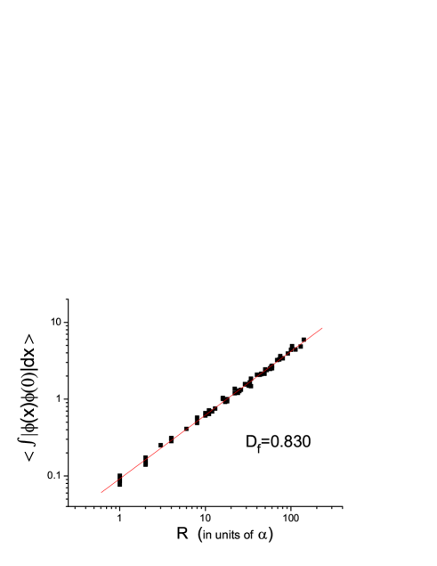
Figure 3: $\langle\int_{R}|\varphi(x)\varphi(0)|\,dx\rangle$ versus $R$ for the ensemble of $\varphi$-field configurations. The slope, i.e the fractal mass dimension $D_{f}$, is equal to $5/6$ within an error of less than 0.3%.

the slope, i.e the fractal mass dimension $D_{f}$ according to (15), is equal to $5/6$ within an error of less than 0.3%.

III.2 Higher Dimensional Case

The higher dimensional generalization of our algorithm is straightforward, preserving the improved mean field approach using piecewise constant configurations. For $D>1$ we use configurations consisting of $D-$dimensional boxes as basis and the ensemble production is reduced to the Cartesian product of the one dimensional case. Finally, the decisive test about the proper configuration production will be the calculation of the fractal mass dimension (10), as in the $1-D$ case. In particular the $3-D$ case is physically very interesting since the effective action (2) describes the order parameter dynamics of the Ising universality class at the spontaneous magnetization transition point. Thus, contrary to the one dimensional case, the investigated $3-D$ system has a physical impact describing the standard model of a very common critical state.

We firstly perform a random partitioning of the $D-$dimensional lattice in a random integer number of elementary box-shaped clusters of different volume, each one consisting of several lattice points. This is succeeded by applying the $1-D$ partitioning algorithm $D$ times and then taking the Cartesian product of the $1-D$ partitions. In this case the linear size of the lattice is reduced, leading to a significant decrease of the partitioning algorithm computational time. For example, the time needed for the partitioning of a $20\times 20\times 20$ lattice is two orders of magnitude smaller than that of a $2000-$site linear lattice.

Similarly to the $1-D$ case, we assign a random constant value of the field (in the interval $[-\varphi_{max},+\varphi_{max}$]) to the lattice sites within each cluster, and for this piecewise constant configuration we calculate the $D$-dimensional effective action (2), using the corresponding generalized formula of eq. (13). The sum extends to every lattice site using periodic boundary conditions, and the derivative is calculated using the straightforward $D$-dimensional generalization. The value of the coupling $g$ in the $3-D$ Ising effective action has been determined in the literature ($g\approx 2$ Tetrad02 ; Tsypin94 ) and the parameters $\varphi_{max}$, $k_{iter}$ and $l_{iter}$ are determined following the corresponding $1-D$ steps. The only complication enters in the specification of $\varphi_{max}$, which requires the construction of the plot $\langle|\varphi|\rangle_{i}$ versus lattice site $i$, as we have mentioned in the previous subsection, becoming computationally much more demanding in this higher dimensional case.

As a next step, we randomly change the field value of the first box-shaped cluster, we recalculate the effective action and using the same criteria as in the $1-D$ case either we accept or reject the new field value of the first cluster. We perform these steps until we have covered the whole lattice, and we iterate this procedure $k_{iter}$ times, in the end of which we record one field configuration. Repetition of the above algorithm will form the whole ensemble of the field configurations. Finally, our comment in the $1-D$ treatment about the multiple use of a specific lattice partition, holds in the present case, too. However, due to the significantly smaller partitioning computational time, such a treatment is not necessary.

This is the generalized algorithm of producing an ensemble of $D$-dimensional field configurations generating a random fractal measure on the lattice. The ensemble possesses the property of eqs. (10) and (9), where now the fractal mass dimension is determined by the power-law behavior of $m(R)$ around $\vec{x}_{0}=\vec{0}$, averaged inside clusters of volume $V$. Similarly to the $1-D$ case, to acquire the $\langle\int_{R}|\varphi(\vec{x})\varphi(\vec{0})|\,d^{D}x\rangle$ versus $R$ figure we chose $\vec{x}_{0}=\vec{0}$ of a specific configuration, we find $R$ of the cluster to which it belongs, approximated as $\propto\sqrt[D]{V}$, and we calculate the integral $\int|\varphi(\vec{x})\varphi(\vec{0})|\,d^{D}x$, thus obtaining one point in the $\langle\int_{R}|\varphi(\vec{x})\varphi(\vec{0})|\,d^{D}x\rangle$ vs $R$ figure. Repetition of this procedure for the whole configuration ensemble provides all the points in Fig. 4.

As an application we produce an ensemble of $10^{4}$ 3-dimensional field configurations on a $20\times 20\times 20$ lattice, using $\delta=5$ and $g=2$ Tetrad02 ; Tsypin94 . As already discussed, this choice has a physical correspondence, since for dimensionality $D=3$, isothermal critical exponent $\delta=5$ and coupling $g=2$, the free energy (2) describes the effective action of the $3-D$ Ising model at its critical point. In this case, the theoretical value of the fractal mass dimension according to (11) is $5/2$.

In Fig. 4 we observe that in the log-log plot of $\langle\int_{R}|\varphi(\vec{x})\varphi(\vec{0})|\,d^{3}x\rangle$ vs $R$, the slope, i.e the fractal mass dimension $D_{f}$ according to (9), is equal to $5/2$, within an error of less than 1%.

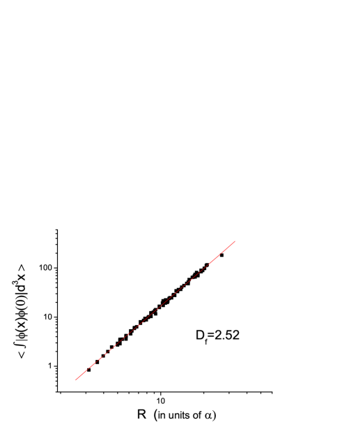
Figure 4: $\langle\int_{R}|\varphi(\vec{x})\varphi(\vec{0})|\,d^{3}x\rangle$ versus $R$ for the ensemble of $3-D$ $\varphi$-field configurations. The slope, i.e the fractal mass dimension $D_{f}$, is equal to $5/2$ within an error of less than 1%.

In order to test that the proposed algorithm is valid for any lattice site, as dictated by the statistics in the considered system, we have calculated $D_{f}$ using different reference points $\vec{x}_{0}$ (sources in (3)) on the $3-D$ lattice. The corresponding distribution $\rho(D_{f})$ is shown in Fig. 5.

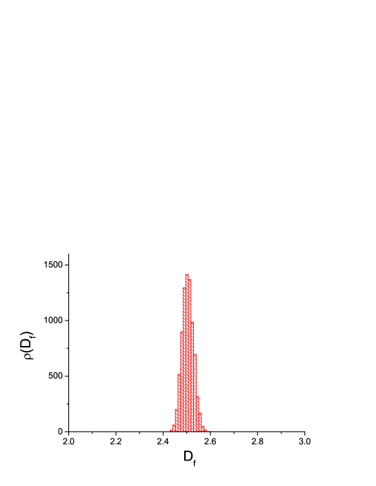
Figure 5: $\rho(D_{f})$ calculated using $8\times 10^{3}$ different reference points $\vec{x}_{0}$ on the lattice.

It is clearly seen that $D_{f}$ is almost constant with a deviation of at most $4\%$ for the given lattice size $N^{3}$, and as we have tested, increasing $N$ this deviation decreases algebraically.

Finally, a last test is performed in order to check the ability of the obtained ensemble of configurations to reproduce the statistical properties of the critical system. Besides the underlying fractal geometry of the critical clusters, the two-point correlation function:

$$C(x,y)=\langle|\varphi(x)\varphi(y)|\rangle-\langle|\varphi(x)|\rangle\langle|\varphi(y)|\rangle$$ (17)

possesses an analytically known power-law form at the critical point. Using the constructed ensemble of configurations we have calculated numerically the correlation function (17) and the result is shown in Fig. 6. The theoretical expectation $C(x,y)\sim|x-y|^{-1-\eta}$ ($\eta\approx 0.04$ for the $3-D$ Ising universality class), corrected by a small exponential factor incorporating finite size effects, is shown with the dashed line. It is clearly seen that the calculated $C(x,y)$ is in very good agreement with the analytical formula supporting further the equivalence of the obtained ensemble of configurations with the critical state of the considered system.

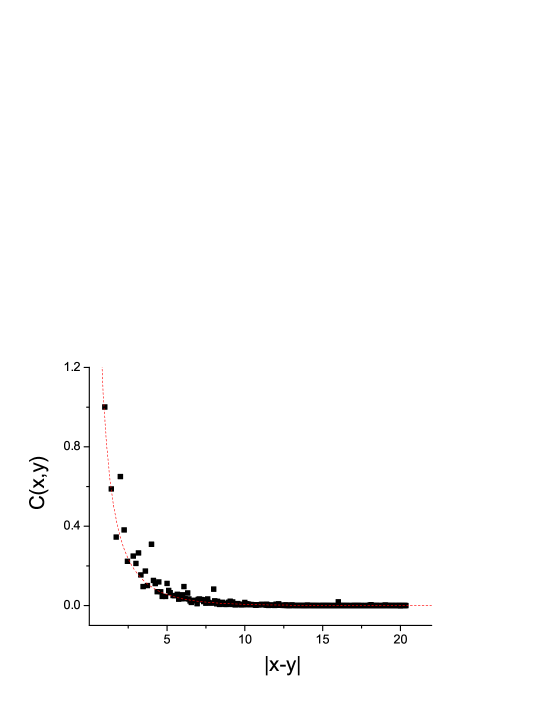
Figure 6: $C(x,y)$ as a function of $|x-y|$ calculated using $10^{4}$ critical configurations for the $3-D$ one-component real scalar field (Ising). The dashed line presents the theoretically expected result.

IV Concluding remarks

Using the saddle-point approach introduced in Anton98 we have been able to develop an algorithm simulating the critical state of a macroscopic system at its transition point. The method followed here is in close analogy with the improved mean field theory imprmeanfield and leads to a successful and computationally efficient description of the geometrical characteristics of the critical clusters, defining suitable measures to quantify this property. A particularly appealing issue of the proposed method is that it provides a link between the effective action at the critical point and the fractal geometry of the formed clusters, overcoming the huge numerical effort needed for the detailed description of fractal sets. Thus, it is the first time, at least to our knowledge, that geometrical characteristics as well as statistical properties of the critical system, are incorporated in an ensemble of configurations suitable for the study of any desired observable at the critical point. The proposed algorithm may be of special interest for the treatment of systems where the formed critical state is not observable but acts as an intermediate state for the subsequent evolution of the system. Such a scenario is likely to hold in the collision of two heavy nuclei at high energies RW00 when the formed fireball freezes out near the theoretically predicted QCD critical point.

Acknowledgements:

We thank N. Tetradis for useful discussions. One of us (E.N.S) wishes to thank the Greek State Scholarship’s Foundation (IKY) for financial support. The authors acknowledge partial financial support through the research programs “Pythagoras” of the EPEAEK II (European Union and the Greek Ministry of Education) and “Kapodistrias” of the Research Committee of the University of Athens.

References

- (1) M. E. J. Newman and G. T. Barkema, Monte Carlo Methods in Statistical Physics, Oxford University Press (1999).
- (2) N. Tetradis, C. Wetterich, Nucl.Phys. B 422, 541 (1994)[arXiv:hep-ph/9308214 v1].
- (3) R. Fukuda, E. Kyriakopoulos, Nucl.Phys. B 85, 354 (1975).
- (4) J. Berges, N. Tetradis, C. Wetterich, Phys. Rep. 363, 223 (2002).
- (5) M. M. Tsypin, Phys. Rev. Lett. 73, 2015 (1994).
- (6) B. B. Mandelbrot, The Fractal Geometry of Nature, W. H. Freeman and Company, New York (1983).
- (7) P. A. Alemany and D. H. Zanette, Phys. Rev. E 49, R956 (1994).
- (8) J. M. Blackledge, A. K. Evans,M. J. Turner Fractal Geometry: Mathematical Methods, Algorithms, Application , Horwood Publishing, (2004).
- (9) H. E. Stanley, Introduction to Phase Transitions and Critical Phenomena , Oxford University Press, New York (1971).
- (10) N. G. Antoniou, F. K. Diakonos, E. N. Saridakis, G. A. Tsolias, [arXiv:physics/0512053].
- (11) D. R. Chialvo, Nature Phys. 2, 301 (2006).
- (12) R. E. Peierls, Surprises in Theoretical Physics, Princeton University Press, Princeton, NJ (1979).
- (13) N. G. Antoniou et al, Phys. Rev. Lett. 81, 4289 (1998) [arXiv:hep-ph/9810383]; N. G. Antoniou, Y. F. Contoyiannis, F. K. Diakonos, Phys. Rev. E 62, 3125 (2000) [arXiv:hep-ph/0008047].
- (14) K. Huang, Statistical Mechanics , John Wiley Sons (1987).
- (15) I. S. Gradshteyn and I. M. Ryzhik, Tables of Integrals, Series and Products, Academic Press, Orlando (1965).
- (16) T. Vicsek, Fractal Growth Phenomena, World Scientific, Singapore (1999).
- (17) K. Falconer, Fractal Geometry: Mathematical Foundations and Applications, John Wiley & Sons, West Sussex (2003).
- (18) R. B. Stinchcombe, Order and Chaos in Nonlinear Physical Systems, Plenum Press, New York (1988).
- (19) A. Nijenhuis, H. .S .Wilf Combinational Algorithms For Computers And Calculators , Academic Press (1978).
- (20) N. Metropolis et al, J. Chem. Phys. 21, 1087 (1953).
- (21) R. Kikuchi, Phys. Rev. 81, 988 (1951); G. W. Woodbury, J. Chem. Phys. 47, 270 (1967).
- (22) K. Rajagopal and F. Wilczek, At the Frontier of Particle Physics. Handbook of QCD, M. Shifman, ed., (World Scientific) [arXiv:hep-ph/0011333].