Quasi-static non-linear characteristics of double-reed instruments

Abstract

This article proposes a characterisation of the double-reed in quasi-static regimes. The non-linear relation between the pressure drop $\Delta p$ in the double-reed and the volume flow crossing it $q$ is measured for slow variations of these variables. The volume flow is determined from the pressure drop in a diaphragm replacing the instrument’s bore. Measurements are compared to other experimental results on reed instrument exciters and to physical models, revealing that clarinet, oboe and bassoon quasi-static behavior relies on similar working principles. Differences in the experimental results are interpreted in terms of pressure recovery due to the conical diffuser role of the downstream part of double-reed mouthpieces (the staple).

I Introduction

I.1 Context

The usual method for studying and simulating the behavior of self-sustained instruments is to separate them in two functional parts that interact through a set of linked variables: the resonator, typically described by linear acoustics, and the exciter, a non-linear element indispensable to create and maintain the auto-oscillations of the instrument Helmholtz, (1954).

Although this separation may be artificial because there may not be a well-defined boundary between the two systems, it is usually a simplified view that allows to describe the basic functioning principles of the instrument. In reed instruments, for instance, the resonator is assimilated to an air column inside the bore, and the exciter to the reed, which acts as a valve.

In the resonator of wind instruments, the relation between the acoustic variables, pressure ($p$) and volume flow ($q$) can be described by a linear approximation to the acoustic propagation which has no perceptive consequences in sound simulations Gilbert et al., (2005). The oscillation arises from the coupling between the reed and the air column, which is mathematically established through the variables $p$ and $q$.

The exciter is necessarily a nonlinear component, so that the continuous source of energy supplied by the pressure inside the musician’s mouth can be transformed into an oscillating one Helmholtz, (1954) Fletcher and Rossing, (1998). The characterisation of the exciter thus requires the knowledge of the relations between variables $p$ and $q$ at the reed output (the coupling region).

In principle this relation is non-instantaneous, because of inertial effects in the reed oscillation and the fluid dynamics. A first approach to the characterisation of the exciter is thus to restrict the study to cases where these delayed dependencies (or, equivalently, time derivatives in the mathematical description of the exciter) can be neglected.

The aim of this paper is to measure the relation between the pressure and volume flow at the double reed output in a quasi-static case, that is, when the time variations of $p$ and $q$ can be neglected, and to propose a model to explain the measured relation.

I.2 Elementary reed model

In quasi-static conditions, a simple model can be used to describe the reed behavior Wilson and S., (1974). The reed opening area ($S$) is controlled by the difference of pressure on both sides of the reed: the pressure inside the reed ($p_{r}$) and the pressure inside the mouth ($p_{m}$). In the simplest model, the relation between pressure and reed opening area is considered to be linear and related through a stiffness constant ($k_{s}$):

$$(\Delta p)_{r}=p_{m}-p_{r}=k_{S}(S_{0}-S)$$ (1)

In this formula, $S_{0}$ is the reed opening area at rest, when the pressure is the same on both sides of the reed. In most instruments (such as clarinets, oboes or bassoons) the reed is said to be blown-closed (or inward-striking) Helmholtz, (1954), because when the mouth pressure ($p_{m}$) is increased, the reed opening area decreases.

The role of the reed is to control and modulate the volume flow ($q$) entering the instrument. The Bernoulli theorem applied between the mouth and the reed duct determines the velocity of the flow inside the reed ($u_{r}$) independently of the reed opening area:

$$p_{m}+\frac{1}{2}\rho u_{m}^{2}=p_{r}+\frac{1}{2}\rho u_{r}^{2}$$ (2)

In this equation, $\rho$ is the air density. Usually, the flow velocity $u_{m}$ is neglected inside the mouth, because of volume flow conservation: inside the mouth the flow is distributed along a much wider cross-section than inside the reed duct.

The volume flow ($q$) is the integrated flow velocity ($u_{r}$) over a cross-section of the reed duct. For the sake of simplicity, the flow velocity is considered to be constant over the whole opening area, so that $q=Su_{r}$. Using equation (2), the flow is given by

$$q=S\sqrt{\frac{2(p_{m}-p_{r})}{\rho}}$$ (3)

Combining eq. (3) and eq. (1), it is possible to find the relation between the variables that establish the coupling with the resonator ($p_{r}$ and $q$):

$$q=\frac{p_{M}-(\Delta p)_{r}}{k_{s}}\sqrt{\frac{2(\Delta p)_{r}}{\rho}}$$ (4)

The relation defined by equation (4) is plotted in figure 1, constituting what we will call the elementary model for the reed.

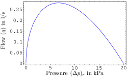
Figure 1: A typical non-linear characteristic curve for a reed of dimensions similar to an oboe reed, given by equation (4)

The static reed beating pressure Dalmont et al., (2005) $p_{M}=k_{s}S_{0}$ is an alternative parameter to $S_{0}$, and can be used as a magnitude for proposing a dimensionless pressure:

$$\tilde{p}=(\Delta p)_{r}/p_{M}$$ (5)

Similarly a magnitude can be found for $q$, leading to the definition of the dimensionless volume flow

$$\tilde{q}=\frac{k_{s}}{p_{M}^{3/2}}\sqrt{\frac{\rho}{2}}q$$ (6)

Equation (4) can then be re-written in terms of these dimensionless quantities:

$$\tilde{q}=(1-\tilde{p})\tilde{p}^{1/2}$$ (7)

This formula shows that the shape of the non-linear characteristic curve of the elementary model is independent of the reed and blowing parameters, although the curve is scaled along the pressure $p$ and volume flow $q$ axis both by the stiffness $k_{s}$ and the beating pressure $p_{M}=k_{s}S_{0}$.

I.3 Generalisation to double-reeds

For reed instruments, the quasi-static non-linear characteristic curve has been measured in a clarinet mouthpiece Backus, (1963), Dalmont et al., (2003), and the elementary mathematical model described above can explain remarkably well the obtained curve almost until the reed beating pressure ($p_{M}$).

For double-reed instruments it was not verified that the same model can be applied. In fact, there are some geometrical differences in the flow path that can considerably change the theoretical relation of equation (7). Local minima of the reed duct cross-section may cause the separation of the flow from the walls and an additional loss of head of the flow Wijnands and Hirschberg, (1995), and in that case the characteristics curve would change from single-valued to multi-valued in a limited pressure range. This kind of change could have significant consequences on the reed oscillations.

However, the non-linear characteristic relation was never measured before for double-reeds, justifying the work that is presented below.

II Principles of measurement and practical issues

The characteristic curve requires the synchronised measurement of two quantities: the pressure drop across the reed $(\Delta p)_{r}$ and the induced volume flow $q$.

II.1 Volume flow measurements

One of the main difficulties in the measurement of the reed characteristics lies in the measurement of the volume flow. There are instruments which can accurately measure the flow velocity in an isolated point (LDA, hot-wire probes) or in a region of a plane (PIV), but it can be difficult to calculate the corresponding flow by integrating the velocity field. In fact it is difficult to do a sampling of a complete cross-section of the reed because a large number of points would have to be registered. Supposing that the flow is axisymmetric at the reed output (which is confirmed by experimental results Almeida, (2006)), the measurement along a diameter of the reed would be sufficient, but regions close to the wall are inaccessible.

On the other hand, commercial flow-meters usually have the disadvantage of requiring a direct reading, which would have been unpractical for a complete characteristic measurement (large number of readings in a short time interval).

An indirect way of measuring the flow was then preferred to the above mentioned methods. It consists in introducing a flow resistance in series with the reed, for which the pressure can be accurately related to the flow running through it (see fig. 2).

The diaphragm method, used successfully by S. Ollivier Ollivier, (2002) to measure the non-linear characteristic of single reeds, is based on this principle. The resistance is simply a perforated metal disk which covers the reed output.

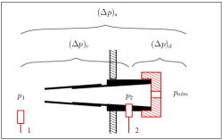
Figure 2: Use of a diaphragm to measure flow and pressure difference in the reed. Numbered rectangles correspond to the pressure probes used in the measurement.

For such a resistance, and assuming laminar, viscous less flow, the pressure drop $\left(\Delta p\right)_{d}=p_{r}-p_{atm}$ across the diaphragm can be approximated by the Bernoulli law :

$$\left(\Delta p\right)_{d}=p_{r}-p_{atm}=\frac{1}{2}\rho\left(\frac{q}{S_{d}}\right)^{2}$$ (8)

where $q$ is the flow crossing the diaphragm, $S_{d}$ the cross section of the hole, and $\rho$ the density of air. In our experiment, pressure $p_{atm}$ is the pressure downstream of the diaphragm (usually the atmospheric pressure, because the flow opens directly into free air). The volume flow $q$ is then determined using a single pressure measurement $p_{r}$.

II.2 Practical issues and solutions

II.2.1 Issues

The realisation of the characteristic measurement experiments encountered two main problems:

Diaphragm reduces the range of $(\Delta p)_{r}$ for which the measurement is possible

The addition of a resistance to the air flow circuit of the reed changes the overall nonlinear characteristic of the reed plus diaphragm system (corresponding to $\left(\Delta p\right)_{s}$ in fig. 2 and to the dashed line in fig. 3). The solid line plots the flow against $\left(\Delta p\right)_{r}$, the pressure drop needed to plot the non-linear characteristics. When the resistance is increased, the maximum value of the system’s characteristic is displaced towards higher pressures Wijnands and Hirschberg, (1995), whereas the static beating pressure ($p_{M}$) value does not change (because when the reed closes there is no flow and the pressure drop in the diaphragm ($\left(\Delta p\right)_{d}$) is zero).

Figure 3: Comparison of the theoretical reed characteristics (solid line) with the a model of the overall characteristics of the reed associated to a diaphragm (dashed) — mathematical models, based on the Bernoulli theorem Wijnands and Hirschberg, (1995).

Therefore, if the diaphragm is too small (i. e., the resistance is too high), part of the decreasing region (B’C) of the system’s characteristics becomes vertical, or even multivalued, so that there is a quick transition between two distant flow values, preventing the measurement of this part of the characteristic curve Dalmont et al., (2003) (see figure 3). A critical diaphragm size ($S_{d,crit}=0.58S_{0}$) can be found below which the characteristic curve becomes multi-valued (see appendix A).

Reed auto-oscillations

Auto-oscillations have to be prevented here to keep consistent with the quasi-static measurement (slow variations of pressure and flow). This proved to be difficult to achieve in practice. In fact, auto-oscillations become possible when the reed ceases to act as a passive resistance (a positive $\frac{\partial q}{\partial p}$, which absorbs energy from the standing wave inside the reed channel) to become an active supply of energy ($\frac{\partial q}{\partial p}<0$). All real acoustic resonators are slightly resistive (the input admittance $Y_{in}$ has a positive real part). This can compensate in part the negative resistance of the reed in its active region, but only below a threshold pressure, where the slope of the characteristic curve is smaller than the real part of $Y_{in}$ for the resonator Debut and Kergomard, (2004).

One way to avoid auto-oscillations is thus to increase the real part of $Y_{in}$, that is the acoustic resistance of the resonator. It is known that a an orifice in an a acoustical duct with a steady flow works as an anechoic termination works as an acoustic resistance Durrieu et al., (2001), so that if the diaphragm used to measure the flow (see sect. II.1) is correctly dimensioned, the acoustic admittance seen by the reed $Y_{in}$ can become sufficiently resistive to avoid oscillations.

II.2.2 Solutions proposed to adress these issues

Size of the diaphragm

The volume flow is determined from the pressure drop across the diaphragm placed downstream of the reed. In practice there’s a tradeoff that determines the ideal size of the diaphragm. If it is too wide, the pressure drop is too small to be measured accurately, and reed oscillations likely to occur. If the diaphragm is too small, the system-wide characteristic can become too steep, making part of the ($(\Delta p)_{r}$) range inaccessible.

The ideal diaphragm cross-section is then found empirically, by trying out several resistance values until one complete measurement can be done without oscillations or sudden closings of the reed. The optimal diaphragm diameter is sought using a medical flow regulator with continuously adjustable cross-section as a replacement for the diaphragm.

Finer control of the mouth pressure $p_{m}$

During the attempts to find an optimal diaphragm, it was found that sudden closures were correlated to sudden increases in the mouth pressure. A part of the problem is that the mouth pressure depends both on the reducer setting [or configuration] and on the downstream resistance. By introducing a leak upstream of the experimental apparatus (thus not altering the experiment) , it is possible to improve measurements in the decreasing region of the characteristic (BC), at least when the system-wide characteristic is not multi-valued (see section II.2.1).

Increase the reed mass

One other way to reduce the oscillations is thus to prevent the appearance of instabilities, or to reduce their effects. An increase in the reed damping would certainly be a good method to avoid oscillations, because it cancels out the active role of the reed (which can be seen as a negative damping) Debut, (2004).

It is difficult to increase the damping of the reed without altering its opening or stiffness properties. The simplest way found to prevent reed oscillations was thus an increase in the reed mass.

This mass increase was implemented by attaching small masses of Blu-Tack to one or both blades of the reed (fig. 4). During measurements on previously soaked reeds it was difficult to keep the masses attached to the reed, so that an additional portion of Blu-Tack is used to connect the to masses together, wrapping around the reed. A comparison of the results using different masses showed that their effect on the quasi-static characteristics can be neglected.

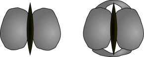
Figure 4: Front view of the reed with attached masses, at left in dry conditions, at right in soaked conditions (to prevent the masses from slipping).

II.3 Experimental set-up and calibrations

The experimental device is shown in figure 5. An artificial mouth Almeida et al., (2004) was used as a blowing mechanism and support for the reed. The window in front of the reed allows the capture of frontal pictures of the reed opening.

Artificial lips, allowing to adjust the initial opening area of the reed were not used here, fearing that they would modify some of the elastic properties of the reed, yet differently from what happens with real lips.

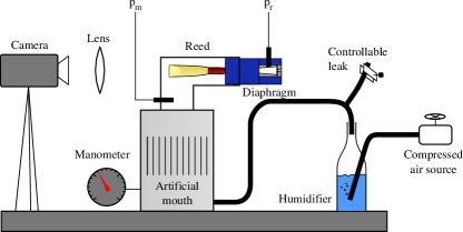
Figure 5: Device used for characteristics measurements.

As stated before, the plot of the characteristic curve requires two coordinated measurements: the pressure difference $(\Delta p)_{r}$ across the reed and the induced volume flow $q$, determined from the pressure drop $(\Delta p)_{d}$ across a calibrated diaphragm (sect. II.1).

In practice thus, the experiment requires two pressure measurements $p_{m}$ and $p_{r}$, as shown in figure 5.

II.3.1 Pressure measurements

The pressure is measured in the mouth and in the reed using Honeywell SCX series, silicon-membrane differential pressure sensors whose range is from $-50$ to $50$ kPa.

These sensors are not mounted directly on the measurement points, but one of the terminals in each sensor is connected to the measurement point using a short flexible tube (about $20$ cm in length). Therefore, one tube opens in the inside wall of the artificial mouth, $4$ cm upstream from the reed, and the other tube crosses the rubber socket attaching the diaphragm to the reed output. The use of these tubes does not influence the measured pressures as long as their variations are slow.

The signal from these sensors is amplified before entering the digital acquisition card. The gain is adjusted for each type of reed. The system consisting of the sensor connected to the amplifier is calibrated as a whole in order to find the voltage at the amplifier output corresponding to each pressure difference in the probe terminals: the stable pressure drop applied to the probe is also measured using a digital manometer connected to the same volumes, and compared to the probe tension read using a digital voltmeter. Voltage is found to vary linearly with the applied pressure within the measuring range of the sensor.

II.3.2 Diaphragm calibration

The curve relating volume flow $q$ to the pressure difference through diaphragms $(\Delta_{p})_{d}$ can be approximated by the Bernoulli theorem. In fact, diaphragms are constructed so as to minimize friction effects (by reducing the length of the diaphragm channel) and jet contraction — the upstream edges are smoothed by chamfering at 45^∘ (fig. 6). The chamfer height ($c$) is approximately 0.5 mm. The diaphragm channel is 3 mm long ($L$).

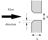
Figure 6: Detail of the diaphragm dimensions.

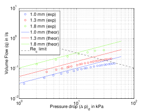
Figure 7: Calibration of diaphragms used in characteristic measurements (dots are experimental data and lines are Bernoulli predictions using the measured diaphragm diameters). The dashed black line represents the pressure/flow relation corresponding to the expected transition between laminar and turbulent flows ($Re_{c}=2000$), parameterised by the diaphragm diameter $d$.

Nevertheless, this ideal characteristic was checked for each diaphragm (see fig 7). It was found that the effective cross-section is slightly smaller than the actual cross-section (about 10%), which is probably due to some Vena Contracta effect in the entrance of the diaphragm. Moreover, above a given pressure drop the volume flow increase is lower than what is predicted by Bernoulli’s theorem (corresponding to a lower exponent than $1/2$ predicted by Bernoulli). This difference is probably due to turbulence generated for high Reynolds Numbers. In figure 7 the dashed line corresponding to the critical value of the Reynolds number ($Re_{c}=\frac{ud}{\nu}=2000$) is shown. It is calculated using the following formulas for $u$ (the average flow velocity in the diaphragm) and $d$ (the diaphragm diameter):

$$d = \left(\frac{2}{\pi}\frac{q}{u}\right)^{1/2}$$ (9)

$$u = \left(\frac{2(\Delta p)_{d}}{\rho}\right)^{1/2}$$ (10)

so that the constant Reynolds relation is given by:

$$Q^{1/2}\Delta p^{1/4}=Re_{c}\nu\left(\frac{\pi}{2}\right)^{1/2}\left(\frac{\rho}{2}\right)^{1/4}$$ (11)

where the right-hand side should be a constant based on the diaphragm geometry.

Since a suitable model was not found for the data displayed in figure 7, we chose to interpolate the experimental calibrations in order to find the flow corresponding to each pressure drop in the diaphragm. Linear interpolation was used in the $(p,q^{2})$ space.

II.3.3 Typical run

In a typical run, the mouth pressure $p_{m}$ is equilibrated with the atmospheric pressure in the room in the beginning of the experiment. Both $p_{m}$ and $p_{r}$ are recorded in the computer through a digital acquisition device at a sampling rate of 4000 Hz. $p_{m}$ is increased until slightly above the pressure at which the reed closes, left for some seconds above this value and then decreased back to the atmospheric pressure. The whole procedure lasts for about 3 minutes, and is depicted in figure 8.

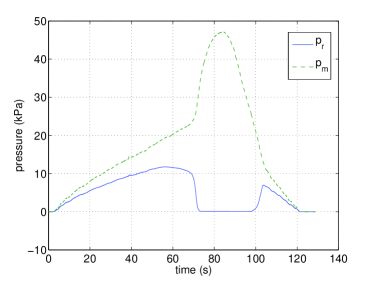
Figure 8: Time variation of the mouth pressure ($p_{m}$)and the pressure inside the reed ($p_{r}$) during a successful characteristic measurement.

II.4 Double-reeds used in this study and operating conditions

Among the great variety of double-reeds that are used in music, we chose as a first target for these measurements a natural cane oboe-reed fabricated using standard procedures (by Glotin), and sold to the oboist (usually a beginner oboist) as a final product (i.e., ready to be played).

The choice of a ready-to-use cane reed was mainly retained because it can be considered as an average reed. This avoids considering a particular scraping technique among many used by musicians and reed-makers. Of course, this does not greatly facilitate the task of the reed measurement, because natural reeds are very sensitive to environment conditions, age or time of usage.

Other reeds were also tested, as a term of comparison with the natural reeds used in most of the experiments. However, none of these reeds was produced by a professional oboist or reed maker, although it would be an interesting project to investigate the variations in reeds produced by different professionals.

To conclude, the results presented in the next section may depend to a certain extent on the reed chosen for the experiments, and a larger sample of reeds embracing the big diversity of scraping techniques needs to be tested before claiming for the generality of the results that will be presented.

Another remark has to be made on the conditions during the experiments. The kind of reeds used in most experiments are always blown with highly moisturised air. In fact, in real life, reeds are often soaked before they are used, and constantly maintained wet by saliva and water vapour condensation. These conditions were sought throughout most of the experiments, although their sensitivity to environmental conditions was also investigated. For instance, the added masses were found to have no practical influence on the nonlinear characteristics, whereas the humidity increases the hysteresis in the complete measurement cycle (increasing followed by decreasing pressures), while reducing the reed opening at rest Almeida, (2006).

In our measurements, humidification is achieved by letting the air flow through a plastic bottle half-filled with hot water at $40^{\circ}$ (see fig. 5), recovering it from the top. Air arriving in the artificial mouth has a lower temperature, because its temperature is approximately $10^{\circ}$ when entering the bottle. This causes the temperature and humidity to decrease gradually along the experiments. Future measurements should include a thermostat for the water temperature in order to ensure stable humidification

III Results and discussion

III.1 Typical pressure vs flow characteristics

Using the formula of eq. (8), and the calibrations carried out for the diaphragm used in the measurement, the flow is determined from the pressure inside the reed ($p_{r}$). The pressure drop in the reed corresponds to the difference between the mouth and reed pressures ($(\Delta p)_{r}=p_{m}-p_{r}$). Volume flow ($q$) is then plotted against the pressure difference ($(\Delta p)_{r}$), yielding a curve shown in figure 9.

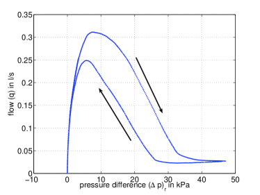
Figure 9: A typical result for the measurement of the volume flow vs pressure characteristic of a natural cane oboe reed.

In this figure, the flow is seen to increase until a certain maximum value (at about 6 kPa). When the pressure is increased further, flow decreases due to the closing of the reed. Instead of completely vanishing for $(\Delta p)_{r}=p_{M}$, as predicted by the elementary model shown in section I.2, the flow first stabilises at a certain minimum value and then increases when the pressure is increased further., indicating that it is very hard to completely close the reed.

The flow remaining after the two blades are in contact suggests that despite the closed apparency of the double reed, some narrow channels remaining between the two blades are impossible to close, behaving like rigid capillary ducts, which is corroborated by the slight increase in the residual volume flow for high pressures.

If the residual reed opening is distributed over several channels, the flow in each of these channels would be controlled by viscosity rather then inertia, so that the volume flow $q$ should be proportional to $(\Delta p)_{r}$ rather than to the $1/2$ power of it as in the case of a Bernoulli flow. Nevertheless, observing a logarithmic plot of the non-linear characteristics (fig. 10) shows a $1/2$ power dependence of the residual flow. This may mean that the reed material is not yet stable at this point.

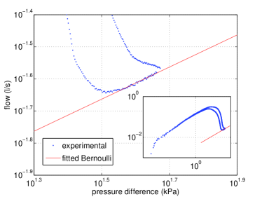
Figure 10: Logarithmic plot of the characteristic curve of figure 9 to show the $1/2$ power dependence when the reed is almost shut.

When reducing the pressure back to zero, the reed follows a different path in the pressure/flow space than the path for increasing pressures. This hysteresis is due to memory effects of the reed material which have been investigated experimentally for single-reed Dalmont et al., (2003) and double-reed instruments Almeida et al., (2006).

III.2 Comparison with other instruments

III.2.1 Bassoon

Since oboes are not the only double-reed instruments, it is interesting to compare the non-linear characteristic curves from different instruments. The bassoon is also played using a double reed, but its dimensions are different: its opening area at rest is typically 7 mm² (against around 2 mm² for the oboe) and the cross section profile varies slightly from oboe reeds.

Figure 11 compares two characteristic curves for natural cane oboe and bassoon reeds. Both were measured under similar experimental conditions, as far as possible. The reed was introduced dry in the artificial mouth, but the supplied air is moisturized at nearly 100% humidity, and masses were added to both reeds to prevent auto-oscillations. The diaphragms used in each measurement are different however, and this is because the opening area of the reed at rest is much larger in the case of the bassoon, so that a smaller resistance (a larger diaphragm) is needed to avoid that the reed closes suddenly in the decreasing side of the characteristic curve (see section II.3 and eq. 27). This should not have any consequences in the measured characteristic curve.

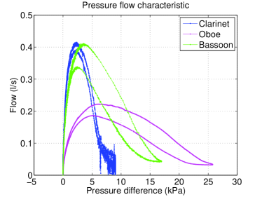
Figure 11: Comparison of the characteristic curves of different reed exciters for different instruments. Clarinet data was obtained by S. Ollivier and J.-P. Dalmont Dalmont et al., (2003) for a PlastiCover®  reed. Oboe and bassoon reeds used moisturised air.

In the $q$ axis, the bassoon reed reaches higher values, and this is probably a consequence of its larger opening area at rest, although the surface stiffness is likely to change as well from the oboe to the bassoon reed. In the $p$ axis, the bassoon reed extends over a smaller range of pressures so that the reed beating pressure is about 17 kPa in the case of the bassoon reed whereas it is near 33 kPa for the oboe reed.

Apart from these scaling considerations, the shape of the curves are similar and this can be better observed if flow and pressure are normalized using the maximum flow point of each curve (figure 12).

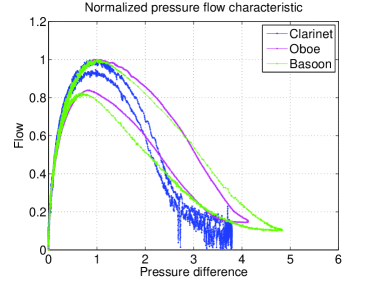
Figure 12: Normalized data from figure 11

III.2.2 Clarinet

The excitation mechanism of clarinets and saxophones share the same principle of functioning with double reeds. However, there are several geometric and mechanical differences between single reeds and double reeds. For instance, flow in a clarinet mouthpiece encounters an abrupt expansion after the first 2 or 3 millimeters of the channel between the reed and the rigid mouthpiece, and the single reed is subject to fewer mechanical constraints than any double reed. These differences suggest that the characteristic curve of single-reed instruments might present some qualitative differences with respect to the double reed Vergez et al., (2003).

The non-linear characteristic curve of clarinet mouthpieces displayed in figures 11 and 12 was measured by S. Ollivier an J.-P. Dalmont Dalmont et al., (2003) using similar methods as the ones we used for the double reed. A comparison between the curves for both kinds of exciters (in figure 11) shows that the overall behavior of the excitation mechanism is similar in both cases. Similarly to when comparing oboe to bassoon reeds, the scalings of the characteristic curves of single-reeds are different from those of oboe reeds, although closer to those of the bassoon. This is probably a question of the dimensions of the opening area.

A different issue is the relation between reference pressure values in the curve (shown in the adimensionalized representation of figure 12). As predicted by the elementary model described in section I.2, in the single reed the pressure at maximum flow is about $1/3$ of the beating pressure of the reed, whereas in double-reed measurements, the relation seems to be closer to $1/4$. This deviation from the model is shown in section IV to be linked with the diffuser effect of the conical staple in double-reeds.

Figure 12 also shows that in the clarinet mouthpiece used by S. Ollivier and J. P. Dalmont the hysteresis is relatively less important than in both kinds of double-reeds. In fact, whereas the measurements for double-reeds were performed in wet conditions, the PlastiCover® reed used for the clarinet was especially chosen because of its smaller sensitivity to environment conditions.

IV Analysis

IV.1 Comparison with the elementary model

The measured non-linear characteristic curve of figure 9 can be compared to the model described in section I.2. In this model, two parameters ($k_{s}$ and $S_{0}$) control the scaling of the curve along the $p$ and $q$ axis. They are used to adjust two key points in the theoretical curve to the experimental one: the reed beating pressure $p_{M}$ and the maximum volume flow $q_{\mathrm{max}}$.

Once $q_{\mathrm{max}}$ is determined through a direct reading, the stiffness $k_{s}$ is calculated using the following relation:

$$k_{s}=q_{\mathrm{max}}^{-1}\left(\frac{2}{3}p_{M}\right)^{3/2}\rho^{-1/2}$$ (12)

This allows to adjust a theoretical characteristic curve (corresponding to the elementary model of equation (4)) to each of the branches of the measured characteristic curve, for increasing and decreasing pressures (fig. 13).

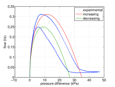
Figure 13: Comparison of the experimental non-linear characteristics curve with the elementary model shown in figure 1. Two models are fitted, for increasing ($p_{M}=35$ kPa, $k_{s}=1.04\times 10^{10}$ kg m^-3 s^-2) and decreasing ($p_{M}=27$ kPa, $k_{s}=8.86\times 10^{9}$ kg m^-3 s^-2) mouth pressures.

When compared to the elementary model of section I.2, the characteristic curve associated to double-reeds shows a deviation of the pressure at which the flow reaches its maximum value. In fact, it can be easily shown that for the elementary model this value is $1/3$ of the reed beating pressure $p_{M}$, which is also verified in the clarinet (sect. III.2.2). In the measured curves however, this value is usually situated between $1/4p_{M}$ and $1/5p_{M}$.

Nevertheless, the shapes of the curves are qualitatively similar to the theoretical ones.

IV.2 Conical diffuser

The former observations about the displacement of the maximum value can be analysed in terms of the pressure recoveries due to flow decelerations inside the reed duct. Variations in the flow velocity are induced by the increasing cross-section of the reed towards the reed output (fig. 14). This can be understood simply by considering energy and mass conservation between two different sections of the reed:

$$p_{in}+\frac{1}{2}\rho\left(\frac{q}{S_{in}}\right)^{2}=p_{out}+\frac{1}{2}\rho\left(\frac{q}{S_{out}}\right)^{2}$$ (13)

where $q$ is the total volume flow that can be calculated either at the input or the output of the conical diffuser by integrating the flow velocity over the cross-section $S_{in}$ or $S_{out}$ respectively.

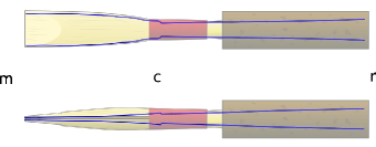
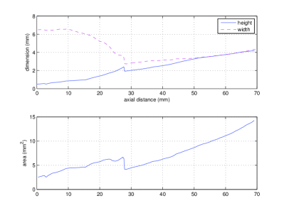
Figure 14: Cross-section profiles (axis and area) of an oboe reed, measured on a mold of the reed channel, and indexes used in section IV.2: mouth, constriction and reed output.

In practice however, energy is not expected to be completely conserved along the flow because of its turbulent nature. In fact, for instance at the reed output (diameter $d$), the Reynolds number of the flow ($Re=\frac{ud}{\nu}=4\frac{q}{\pi d\nu}$) can be estimated using data from figure 9 to reach a maximum value of 5000. Given that this number is inversely proportional to the diameter of the duct $d$, the Reynolds increases upstream, inside the reed duct, so that the flow is expected to be turbulent also for lower volume flows.

For turbulent flows, no theoretical model can be applied to calculate the pressure recovery due to the tapering of the reed duct. However, phenomenological models are available in engineering literature, where similar duct geometries are known as “conical diffusers”. Unlike in clarinet mouthpieces, where the sudden expansion of the profile is likely to cause a turbulent mixing without pressure recovery Hirschberg, (1995), this effect must be considered in conical diffusers. The pressure recovery is usually quantified in terms of a recovery coefficient $C_{P}$ stating the relation between the pressure difference between both ends of the diffuser and the ideal pressure recovery which would be achieved if the flow was stopped without losses:

$$C_{P}=\frac{p_{\mathrm{out}}-p_{\mathrm{in}}}{\frac{1}{2}\rho u_{\mathrm{in}}^{2}}$$ (14)

$C_{P}$ values range from $0$ (no recovery) to $1$ (complete recovery, never achieved in practice). Distributed losses due to laminar viscosity along the reed are neglected.

According to equation (14), pressure recovery is proportional to the square of the flow velocity at the entrance of the conical diffuser, and consequently to the squared volume flow inside the reed. This is coherent with the shifting of the double-reed non-linear characteristics curve for high volume flows, as observed in figure 13.

IV.2.1 Reed model with pressure recovery

In order to take into account the pressure recovery before the reed output, the flow is divided into two sections, the upstream, until the constriction at 28 mm (index $c$ in fig. 14) and the conical diffuser part from the constriction until the reed output. In the upstream section, no pressure recovery is considered, so that the flow velocity can be calculated using the pressure difference between the mouth and this point using a Bernoulli model, as in equation (3), but replacing $p_{r}$ with $p_{c}$:

$$q=S\sqrt{\frac{2(p_{m}-p_{c})}{\rho}}$$ (15)

Similarly, the reed opening is calculated using the same pressure difference:

$$(\Delta p)_{c}=p_{m}-p_{c}=k_{S}(S_{0}-S)$$ (16)

The total pressure difference used to plot the characteristic curve, however, is different, because the recovered pressure has to be added to $(\Delta p)_{c}$:

$$p_{m}-p_{r}=(\Delta p)_{c}-C_{p}\frac{1}{2}\rho\left(\frac{q}{S_{c}}\right)^{2}$$ (17)

where $S_{c}$ is the reed duct cross-section at the diffuser input i. e., at the constriction, which is found from figure 14, $S_{c}=4\times 10^{-6}$ m².

Using these equations, the modified model can be fitted to the experimental data. In figure 15, the same parameters $k_{s}$ and $S_{0}$ were used as in figure 13, leaving only $C_{p}$ as a free parameter for the fitting. Figure 15 was obtained for a value of $C_{p}=0.8$.

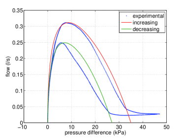
Figure 15: Comparison of the experimental non-linear characteristics curve with a reed model with pressure recovery in the final part of the duct. Fitted $k_{s}$ and $S_{0}$ are the same as in figure 13 and different for increasing and decreasing mouth pressures. In both cases the value $C_{p}=0.8$ was used.

This value can be compared to typical values of pressure recovery coefficients found in industrial machines, for example in Azad, (1996).

In engineering literature, $C_{P}$ is found to depend mostly on the ratio between output and input cross-sections ($AR=S_{\mathrm{out}}/S_{\mathrm{in}}$) and the diffuser length to initial diameter ratio ($L/d_{\mathrm{in}}$) White, (2001). The tapering angle $\theta$ influences the growth of the boundary layers, so that above a critical angle ($\theta=8^{\circ}$) the flow is known to detach from the diffuser walls considerably lowering the recovered pressure. An in-depth study of turbulent flow in conical diffusers can be found in the literature Azad, (1996) usually for diffusers with much larger dimensions than the ones found in the double reed.

The geometry of the conical diffuser studied in Azad, (1996) can be compared to the one studied in our work: the cross-section is circular and the tapering angle $\theta=3.94^{\circ}$ is not very far from the tapering angle of the reed staple $\theta=5.2^{\circ}$ (in particular, both are situated in regions of similar flow regimes Kilne and Abbott, (1962) as a function of the already mentioned $AR$ and $L/d_{\mathrm{in}}$). Reynolds numbers of his flows ($Re=6.9\times 10^{4}$) are also close to the maximum ones found at the staple input ($Re\simeq 10^{4}$).

The length to input diameter ratio of the reed staple $L/d=20$ is bigger than that found in Azad, (1996), however the pressure recovery coefficient can be extrapolated from his data to find the value $C_{P}\simeq 0.8$ (fig. 2 in Azad, (1996)).

V Conclusion

The quasi-static non-linear characteristics was measured for double reeds using a similar device as for single-reed mouthpieces Dalmont et al., (2003). The obtained curves are close to the ones found for single-reeds, and in particular no evidence of multivalued flows for a same pressure was found, as was suggested by some theoretical considerations Wijnands and Hirschberg, (1995), Vergez et al., (2003).

Double-reed characteristic curves present substantial quantitative differences for high volume flows when compared to elementary models for the reed. These differences can be explained using a model of pressure recovery in the conical staple, proportional to the input flow velocity.

It is worth noting that direct application of this measurement to the modelling of the complete oboe is not that obvious. Indeed, the assumption that the mouthpiece as a whole (reed plus staple) can be modelled as a non-linear element with characteristics given by the above experiment would be valid if the size of the mouthpiece was negligible with respect to a typical wavelength. Given the 7 cm of the mouthpiece and the 50 cm of a typical wavelength, this is questionable. Should the staple be considered as part of the resonator? In that case, the separation between the exciter and the resonator would reveal a longuer resonator and an exciter without pressure recovery. This could be investigated through numerical simulations by introducing the pressure recovery coefficient ($C_{P}$) as a free parameter.

Moreover, the underlying assuption of the models is that non stationnary effects are negligible (all flow models are quasi-static). Some clues indicate that this could also be put into question:

• First of all, experimental observations of the flow at the output of the staple (through hot-wire measurements Almeida, (2006)) revealed significant differences in the flow patterns when considering static and auto-oscillating reeds.

• Moreover, non-dimensional analysis reveal Strouhal numbers much larger than for simple reed instruments (Vergez et al., (2003), Almeida, (2006))

Appendix A Calculation of the minimum diaphragm cross-section

The total pressure drop in the reed-diaphragm system (fig. 2) is:

$$(\Delta p)_{s}=(\Delta p)_{r}+(\Delta p)_{d}$$ (18)

The system’s characteristics becomes multivalued when there is at least one point on the curve where the slope is infinite:

$$\frac{\partial}{\partial q}(\Delta p)_{s}=\frac{\partial}{\partial q}(\Delta p)_{r}+\frac{\partial}{\partial q}(\Delta p)_{d}=0$$ (19)

Because of simplicity, the derivatives in equation (18) are replaced by their inverse:

$$\frac{\partial}{\partial q}(\Delta p)_{s}=\left(\frac{\partial q}{\partial(\Delta p)_{r}}\right)^{-1}+\left(\frac{\partial q}{\partial(\Delta p)_{d}}\right)^{-1}=0$$ (20)

yielding

$$\left(\frac{S}{\rho}\left(\frac{2(\Delta p)_{r}}{\rho}\right)^{-1/2}-\frac{1}{k_{s}}\left(\frac{2(\Delta p)_{r}}{\rho}\right)^{1/2}\right)^{-1}+$$

$$+\frac{\rho}{S_{d}}\left(\frac{2(\Delta p)_{d}}{\rho}\right)^{1/2}=0$$ (21)

Solving for $S_{d}$:

$$S_{d} = -\left(\frac{2(\Delta p)_{d}}{\rho}\right)^{1/2}\times$$ (22)

$$\times \left(\frac{S}{\rho}\left(\frac{2(\Delta p)_{r}}{\rho}\right)^{-1/2}-\frac{1}{k_{s}}\left(\frac{2(\Delta p)_{r}}{\rho}\right)^{1/2}\right)$$

Simplifying

$$S_{d}=-S\left(\frac{(\Delta p)_{d}}{(\Delta p)_{r}}\right)^{1/2}+\frac{2}{k_{s}}\left((\Delta p)_{d}(\Delta p)_{r}\right)^{1/2}$$ (23)

From equations (3) and (8), we can find

$$(\Delta p)_{r}=\left(\frac{S_{d}}{S}\right)^{2}(\Delta p)_{d}$$ (24)

and equation (23) can be written

$$S_{d}=-S\frac{S}{S_{d}}+\frac{2}{k_{s}}\frac{S}{S_{d}}(\Delta p)_{r}$$ (25)

Now we can replace $S=S_{0}-\frac{(\Delta p)_{r}}{k_{s}}$ to find

$$S_{d}^{2}=(-S_{0}+3\frac{(\Delta p)_{r}}{k_{s}})(S_{0}-\frac{(\Delta p)_{r}}{k_{s}})$$ (26)

It is clear that the right-hand side of this equation must be positive. Moreover, it is a parabolic function of $(\Delta S)=\frac{(\Delta p)_{r}}{k_{s}}$, with its concavity facing downwards.

The maximum value of $S_{d}^{2}(S)$:

$$\mathrm{max}\left(S_{d}^{2}(S)\right)=\frac{S_{0}^{2}}{3}$$ (27)

is thus the value for which there is only a single point where the characteristic curve has an infinite slope.

We thus conclude that $S_{d}=\frac{S_{0}}{\sqrt{3}}=0.58S_{0}$ is the minimum value of the diaphragm cross-section that should be used for flow measurements.

References

- (1) Static beating pressure: The minimum pressure for which the reed channel is closed.
- (2) The flow velocity at the reed output is neglected when compared to the velocity inside the diaphragm ().
- (3) A plastic adherent material usually used to fixate paper to a wall.
- Almeida, (2006) Almeida, A. (2006). Physics of double-reeds and applications to sound synthesis. PhD thesis, Univ. Paris VI. (to be held in June 2006).
- Almeida et al., (2006) Almeida, A., Vergez, C., and Caussé, R. (2006). Experimental investigation of reed instrument functionning through image analysis of reed opening. Submitted to Acustica.
- Almeida et al., (2004) Almeida, A., Vergez, C., and Caussé, R. (2004). Experimental investigations on double reed quasi-static behavior. In Proceedings of ICA 2004, volume II, pages 1229–1232.
- Azad, (1996) Azad, R. S. (1996). Turbulent flow in a conical diffuser: a review. Exp. Thermal and Fluid Science, 13:318–337.
- Backus, (1963) Backus, J. (1963). Small-vibration theory of the clarinet. Journal of the Acoustical Society of America, 35(3):305–313.
- Dalmont et al., (2005) Dalmont, J.-P., Gilbert, J., Kergomard, J., and Ollivier, S. (2005). An analytical prediction of the oscillation and extinction thresholds of a clarinet. J. Acoust. Soc. Am., 118(5):3294–3305.
- Dalmont et al., (2003) Dalmont, J. P., Gilbert, J., and Ollivier, S. (2003). Nonlinear characteristics of single-reed instruments: quasi-static volume flow and reed opening measurements. J. Acoust. Soc. Am., 114(4):2253–2262.
- Debut, (2004) Debut, V. (2004). Deux études d’un instrument de musique de type clarinette :Analyse des fréquences propres du résonateur et calcul des auto-oscillations par décomposition modale. PhD thesis, Université de la Mediterranée Aix Marseille II.
- Debut and Kergomard, (2004) Debut, V. and Kergomard, J. (2004). Analysis of the self-sustained oscillations of a clarinet as a van-der-pol oscillator. In Proceedings of ICA 2004, volume II, pages 1425–1428.
- Durrieu et al., (2001) Durrieu, P., Hofmans, G., Ajello, G., Boot, R., Aurégan, Y., Hirschberg, A., and Peters, M. C. A. M. (2001). Quasisteady aero-acoustic response of orifices. J. Acoust. Soc. Am., 110(4):1859–1872.
- Fletcher and Rossing, (1998) Fletcher, N. H. and Rossing, T. D. (1998). The Physics of Musical Instruments. Springer-Verlag, 2 edition.
- Gilbert et al., (2005) Gilbert, J., Dalmont, J.-P., and Guimezanes, T. (2005). Nonlinear propagation in woodwinds. In Forum Acusticum 2005, pages 1369–1372.
- Helmholtz, (1954) Helmholtz, H. e. t. b. A. E. (1954). On the Sensations of Tone as a Physiological Basis for the Theory of Music. Dover.
- Hirschberg, (1995) Hirschberg, A. (1995). Mechanics of Musical Instruments, chapter 7: Aero-acoustics of Wind Instruments, pages 229–290. Springer-Verlag.
- Kilne and Abbott, (1962) Kilne, S. J. and Abbott, D. E. (1962). Flow regimes in curved subsonic diffusers. J. Basic Eng., 84:303–312.
- Ollivier, (2002) Ollivier, S. (2002). Contribution à l’étude des Oscillations des Instruments à Vent à Anche Simple. PhD thesis, Université du Maine, Laboratoire d’Acoustique de l’Université du Maine – UMR CNRS 6613.
- Vergez et al., (2003) Vergez, C., Almeida, A., Causse, R., and Rodet, X. (2003). Toward a simple physical model of double-reed musical instruments: Influence of aero-dynamical losses in the embouchure on the coupling between the reed and the bore of the resonator. Acustica, 89:964–973.
- White, (2001) White, F. M. (2001). Fluid Mechanics. McGraw-Hill, 4th edition.
- Wijnands and Hirschberg, (1995) Wijnands, A. P. J. and Hirschberg, A. (1995). Effect of a pipe neck downstream of a double reed. In Proceedings of the International Symposium on Musical Acoustics, pages 149–152. Societe Française d’Acoustique.
- Wilson and S., (1974) Wilson, T. A. and S., B. G. (1974). Operating modes of the clarinet. Jour. Acoust. Soc. Am., 56(2):653–658.