Modeling Society with Statistical Mechanics:
an Application to Cultural Contact and Immigration

Abstract

We introduce a general modeling framework to predict the outcomes, at the population level, of individual psychology and behavior. The framework prescribes that researchers build a cost function that embodies knowledge of what trait values (opinions, behaviors, etc.) are favored by individual interactions under given social conditions. Predictions at the population level are then drawn using methods from statistical mechanics, a branch of theoretical physics born to link the microscopic and macroscopic behavior of physical systems. We demonstrate our approach building a model of cultural contact between two cultures (e.g., immigration), showing that it is possible to make predictions about how contact changes the two cultures.

1 Introduction

Modern society features an increasing degree of interaction between cultures (“cultural contact”) owing to, e.g., communication technologies, immigration and other socio-political forces [Lull (2000)]. In many countries cultural contact is perceived as both an opportunity and a threat and is related to important public issues such as immigration management and the need to “protect” national culture [Cornelius et al. (1994), Givens and Luedtke (2005)]. Our understanding of these phenomena is, however, limited: we cannot predict the outcome of cultural contact, nor make plausible conjectures that can be used in policy making. Within this context, the aim of this paper is twofold: we first describe a general mathematical framework for modeling social interactions, then we make specific assumptions relevant to studying immigration, i.e., social contact between two groups that, typically, differ both in culture and relative size.

2 General framework

2.1 A formalization of social interactions

For simplicity, we focus on a single cultural trait, which may represent an idea, an opinion or a behavior that has two mutually exclusive forms. A useful example to keep in mind is being in favor or against an issue such as the death penalty, or any other issue that might be the subject of a yes/no referendum vote. Our framework allows to consider multiple traits without conceptual differences, although model analysis may in general be much more difficult.

We consider a population of $N$ individuals, labeled by an index $i$ ranging from $1$ to $N$. We associate to the $i$-th individual the variable $s_{i}$, which may take values $+1$ or $-1$ representing the two possible trait values. For instance, $+1$ might represent a yes vote in a referendum, and $-1$ a no vote. The state of the whole population is thus encoded in an array $s$ of $N$ numbers, such as $s=\{+1,-1,+1,\ldots\}$.

The hallmark of social interactions is that individuals may change their opinions or behavior owing to interactions with others. A given couple $(i,k)$ can in principle be in one of the four states $\{+1,+1\}$, $\{-1,+1\}$, $\{+1,-1\}$ and $\{-1,-1\}$, but these outcomes, in general, do not have the same probability. Which one is more likely will depend on the characteristics of individuals such as their culture and personality. Our starting assumption is that individuals have no particular bias towards $+1$ or $-1$ opinions: what matters most is whether, by adopting one or the other value, an individual is in agreement or disagreement with others. There are two reasons for this assumptions. First, social psychologists have shown that, in most cultures, agreement or disagreement with others is a powerful determinant of individual opinions and behavior, often more important than holding a particular opinion [Bond and Smith (1996)]; we will expand on this point in our model of immigration below. Second, our framework allows to introduce biases that favor a particular trait value, if needed. Indeed, any model in which individuals are biased can be recast as a model with unbiased individuals, plus an additional “force” that orients individual opinions. Thus our starting assumption of unbiased individuals does not reduce the generality of the framework. Again, we will make a specific example for the case of immigration below.

To formalize these notions, we assume that individuals take on the trait that minimizes a cost function. We define the cost $H_{ik}$ for individual $i$ to agree or disagree with individual $k$ as

$$H_{ik}(s_{i},s_{k})=-J_{ik}s_{i}s_{k}$$ (1)

where $J_{ik}$ is a number that summarizes the nature of the interaction between $i$ and $k$, as follows. When $i$ and $k$ agree ($s_{i}s_{k}=1$) we have a cost $H_{ik}=-J_{ik}$, while when $i$ and $k$ disagree ($s_{i}s_{k}=-1$) we have $H_{ik}=J_{ik}$. Thus whether agreement or disagreement carries the lesser cost depends on the sign of $J_{ik}$: $J_{ik}>0$ favors agreement while $J_{ik}<0$ favors disagreement. The magnitude of $J_{ik}$ gives how important it is for $i$ to agree or disagree with $j$. If, for instance, $J_{ik}>J_{im}$ then it is more important for $i$ to agree with $k$ than with $m$, while $J_{ik}=0$ means that agreement with $k$ is not relevant to $i$. The signs and magnitudes of the $J_{ik}$’s become important when we consider that an individual interacts with many others. In this case, we assume that the costs $H_{ik}$ relative to each interaction sum up to a total cost $H_{i}$

$$H_{i}(s_{i})=\sum_{k}H(s_{i},s_{k})=-\sum_{k}J_{ik}s_{i}s_{k}$$ (2)

As anticipated above, we can take into account additional factors that may influence individuals modifying equation (2) as follows:

$$H_{i}(s_{i})=-\sum_{k}J_{ik}s_{i}s_{k}-h_{i}s_{i}$$ (3)

meaning that individual $i$ is subject to an additional “force” that favors $s_{i}=1$ if $h_{i}>0$ and $s_{i}=-1$ if $h_{i}<0$. The quantity $h_{i}$ may represent any factor that is not explicitly taken into account by the direct interaction with other individuals. For instance, it may summarize the influence of media, government campaigns or existing culture (see below).

We can now write a population-level cost function as the sum of individual cost functions:

$$H(s)=\sum_{i}H_{i}(s_{i})=-\sum_{i,k}J_{ik}s_{i}s_{k}-\sum_{i}h_{i}s_{i}$$ (4)

We stress that the cost function is a theoretical computational aid to track which trait values are favored by the interactions $J_{ik}$ and the external forces $h_{i}$. We do not assume that individuals explicitly compute or are aware of such costs. Rather, $H(s)$ should be designed so that its minima correspond to those trait values that are favored by the mechanisms with which individuals interact.

2.2 The role of statistical mechanics

Once a cost function has been specified, it is possible to calculate population level quantities such as the average trait value using the methods of statistical mechanics, a branch of theoretical physics. Statistical mechanics was originally concerned with deriving the laws of thermodynamics from the behaviour of atoms and molecules [Thompson (1979)], but can actually be applied to understand the macroscopic (population level) properties of any system composed of many parts that interact according to given microscopic (individual level) rules. More recently its methods have found application in fields as diverse as biology [Mezard et al. (1987)], neuroscience [Amit (1989), Arbib (2003)], economy and finance [Bouchaud and Potters (2000)] and also social science [Durlauf (1999)]. The starting point is to assign to each system configuration $s$ a probability $\Pr(s)$ according to the Boltzmann-Gibbs formula [Thompson (1979)]

$$\Pr(s)=\frac{e^{-H(s)}}{\sum_{s}e^{-H(s)}}$$ (5)

where the sum runs over all possible configurations of the system.In physical applications, the parameter $\beta$ (inverse temperature) usually multiplies $H$ in (5). Here, as in other applications of statistical mechanics such as combinatorial optimization [Mezard et al. (1987)], we include $\beta$ in $H$ itself as an overall scale factor.

By means of (5) a given configuration is considered more or less likely according to whether it is more or less costly: a low value of $H(s)$ results in a high probability of $s$, and vice-versa. Assigning probabilities based on a given cost function is the heart of statistical mechanics and is inspired by the principles of thermodynamics (see the appendix for a short discussion, and th, for a fuller treatment).

Once a probability is assigned to system configurations, it is possible to compute the expected values of quantities of interest and to relate them to the parameters that describe the system. For instance the average cultural trait defined by

$$m(s)=\frac{1}{N}\sum_{i}s_{i}$$ (6)

would have an expected value given by

$$\overline{m}=\sum_{s}m(s)\Pr(s)$$ (7)

Note that, while $m(s)$ is the average trait value in a given configuration, $\overline{m}$ is the average trait value over all possible system configurations, each one weighted according to its probability of occurrence. These probabilities depend on the cost function $H$ and thus on the parameters that appear in its expression, i.e., the $J_{ik}$’s and $h_{i}$’s.

Rather than directly attempting to compute expected values such as (7), statistical mechanics aims to compute the so-called free energy of a system, defined as

$$f=-\log\sum_{s}e^{-H(s)}$$ (8)

The rationale for this strategy is that important quantities such as (7) can be easily computed from knowledge of the free energy function, typically by taking suitable derivatives with respect to system parameters (see appendix). The basic task of statistical mechanics is thus, after the cost function $H$ has been specified, to calculate the free energy function for a given system. We stress that the form of the cost function is not given by statistical mechanics; rather, it is the outcome of a modeling effort relative to a specific problem. We now make an example of how one may proceed.

3 The cultural outcomes of immigration

We illustrate here the potentials of our framework considering the impact of immigration on culture. We consider a large and a small population, which will be referred to, respectively, as residents ($R$) and immigrants ($I$). We let $N_{1}$ be the number of residents, and $N_{2}$ of immigrants, with $N_{1}\gg N_{2}$ and $N=N_{1}+N_{2}$ the total number of individuals. We are interested in how cultural contact changes the average trait values in the two populations, with the aim of understanding the effect of one culture upon the other.

3.1 Interactions between residents and immigrants

Our main assumption regarding how residents and immigrants interact is that people, generally speaking, tend to agree with those who are perceived as similar to oneself and to disagree with those perceived as different. In social psychology this is known as the similarity-attraction hypothesis. It has received ample support, although the details of how we interact with others often depend on social context [Michinov and Monteil (2002), Byrne (1997)]. We consider this assumption a general guideline, and in modeling a specific case it can be modified without difficulty. We formalize the similarity-attraction hypothesis by assuming that high perceived similarity corresponds to positive values of $J_{ik}$, and low perceived similarity to negative values. Since residents and immigrants have generally different cultures, we may assume the following structure for the interaction coefficients $J_{ik}$. We let the interaction between any two residents be $J^{(1,1)}>0$; the similarity-attraction hypothesis suggests that this be a positive number, whose magnitude reflects how strongly residents prefer to agree among themselves. Likewise, we let the interactions between immigrants be $J^{(2,2)}>0$. The mutual interactions $J^{(1,2)}$ and $J^{(2,1)}$ should model whether residents prefer to agree or disagree with immigrants, and vice-versa, and how strongly so. If resident and immigrant cultures are very different, the similarity-attraction hypothesis suggests to take both $J^{(1,2)}$ and $J^{(2,1)}$ as negative, but the best choice of values depends on the specific case one intends to model.

Note that we are assuming that $J_{ik}$ depends only on population membership and not on the particular individuals $i$ and $k$ (the so-called mean field assumption in statistical mechanics). This assumption greatly simplifies mathematical analysis but is not wholly realistic. It can capture the average variation in interactions across population but not the variation that exists within each population. For instance, a more realistic assumption would be to take the $J_{ik}$’s as random variables whose mean and variance depend on population membership. We plan to return on that model (which would represent the two-population generalization of the Sherrington-Kirkpatrick model in statistical mechanics, meza87) in future studies.

When modeling interactions, a technical requirement is that the value of the cost function be proportional to total population size $N$. This guarantees that the free-energy function and important quantities such as average trait value, equation (7), scale appropriately with $N$. In our case the appropriate scaling is $1/2N$, hence the interactions are:

$$J_{ik}=\left\{\begin{array}[]{l@{\qquad}l}\displaystyle\frac{J^{(1,1)}}{2N}&i,k\in R\\ \displaystyle\frac{J^{(1,2)}}{2N}&i\in R,k\in I\\ \displaystyle\frac{J^{(2,1)}}{2N}&i\in I,k\in R\\ \displaystyle\frac{J^{(2,2)}}{2N}&i,k\in I\end{array}\right.$$ (9)

3.2 Modeling pre-existing culture

Before the two populations start to interact, residents and immigrants are each characterized by a given average trait value, say ${\tilde{m}_{1}}$ and ${\tilde{m}_{2}}$, respectively. We consider ${\tilde{m}_{1}}$ and ${\tilde{m}_{2}}$ as experimental data about the beliefs or behavior of each population, which could be obtained from, say, a referendum vote on a particular issue (e.g., the death penalty) or from statistical sampling of the population.

That a population is characterized by a given average value $\tilde{m}_{i}\neq 0$ means that the two forms of the trait are not equally common. Specifically, the individuals with the $+1$ form are $N(1+\tilde{m}_{i})/2$, while $N(1-\tilde{m}_{1})/2$ individuals have the $-1$ form. Pre-existing culture, in other words, is like a bias or force that favors one trait value over the other. For modeling purposes, it is convenient to describe pre-existing culture as a “cultural force” that acts to orient the opinion of otherwise unbiased individuals. This is possible including a force term in the cost function, as shown in (3). By standard methods of statistical mechanics (see appendix) it is possible to show that the force term corresponding to a particular average opinion $\tilde{m}_{i}$ is

$$h^{(i)}=\mathrm{atanh}(\tilde{m}_{i})-J^{(i,i)}\tilde{m}_{i}$$ (10)

where $\mathrm{atanh}$ is the inverse hyperbolic tangent function. To summarize, a model in which individuals are biased so that the average opinion is $\tilde{m}_{i}$ is equivalent to a model with unbiased individuals subject to a force given by (10).

3.3 Model analysis

So far we have specified interaction terms $J_{ik}$ to model cultural contact between two populations and we have introduced equation (10) to represent the pre-existing culture in the two populations. The next step is to compute the average trait values $m_{1}$ and $m_{2}$ in the two populations after immigration has taken place. The same method that allows to derive equation (10) enables us to derive the following equations for $m_{1}$ and $m_{2}$ (see appendix):

$$m_{1}=\tanh\Big{(}(1-\alpha)J^{(1,1)}m_{1}+\alpha(J^{(1,2)}+J^{(2,1)})m_{2}+h^{(1)}\Big{)}$$ (11)

$$m_{2}=\tanh\Big{(}(1-\alpha)(J^{(2,1)}+J^{(1,2)})m_{1}+\alpha J^{(2,2)}m_{2}+h^{(2)}\Big{)}$$ (12)

where $\alpha=N_{2}/N$ is the fraction of immigrants in the total population and $\tanh$ is the hyperbolic tangent function. The values of $m_{1}$ and $m_{2}$ predicted by (3.3) depend of course on values of the $J$ and $h$ parameters, and on $\alpha$. We give here a qualitative description of the different regimes that one can observe varying these parameters. We refer to co for a proof of the following statements, in the context of an analogous model from condensed matter physics.

The two key parameters are $\alpha$, the fraction of immigrants, and the overall scale of the interactions $J_{ik}$, which we label $J$. If $J$ is below a critical value $J^{\star}$, equation (3.3) has always one pair of solutions, for all values of $\alpha$. In this case the two populations are essentially merging into a homogeneous one, with average cultural trait in between the two initial ones—more toward one or the other according to the value of $\alpha$. This regime is not surprising and corresponds to the naïve prediction that one could have made a priori without applying statistical mechanics.

If the interaction scale is large ($J>J^{\star}$), however, model predictions are highly non-trivial, suggesting that the outcome of cultural contact can be surprising. Depending on $J$ there are two critical values for $\alpha$: $\alpha_{1}(J)$ and $\alpha_{2}(J)$ that delimit qualitatively different behavior. For $\alpha\leq\alpha_{1}(J)$ the resident culture dominates dominant and the immigrant culture disappears, i.e., $m_{2}$ is close to $m_{1}$ irrespective of the initial value $\tilde{m}_{2}$. The converse happens when $\alpha\geq\alpha_{2}(J)$, i.e., immigrant culture dominates. The most interesting case occurs when $\alpha_{1}(J)\leq\alpha\leq\alpha_{2}(J)$. In this regime (3.3) has two distinct solutions in which either of the two cultures dominates. That is, both cultures may survive the immigration process, generally with a different probability determined by system parameters.

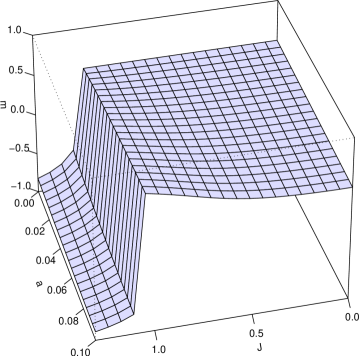
Figure 1: Possible outcomes of cultural contact. Average trait value in the two populations, $m=(1-\alpha)m_{1}+\alpha m_{2}$, is plotted as a function of $\alpha$ (fraction of immigrants) and $J$ (scale of the interaction) for an interaction matrix of the form (9) with $J^{(i,k)}=J$. Before the interaction the two populations have initial trait values of $\tilde{m}_{1}=0.5$ and $\tilde{m}_{2}=-0.5$. Only the most likely outcome is plotted (see text).

The parameter values that favor the resident or immigrant culture, have still to be worked out and will be the topic of future work.As noted above, co has studied a formally identical model arising from a condensed-matter problem, but there the $h_{i}$’s were free parameters, while here they are determined in terms of the $J^{(i,i)}$ and the $\tilde{m}_{i}$ through (10). Here we analyze the case in which the intensity of the interactions is uniform both within and between groups, $J^{(i,k)}=J$. This is interpreted as two groups that do not really discriminate between themselves, so that disagreement with any particular individual carries the same cost independent of which group the individual belongs to. We assume, however, that the two groups have initially a very different average trait value: $\tilde{m}_{1}=0.5$ and $\tilde{m}_{2}=-0.5$. In figure 1 we explore this system by plotting the average trait value after the interaction, $m=(1-\alpha)m_{1}+\alpha m_{2}$, for $\alpha$ between 0 and 10% and for $J\geq 0$.The maximum admissible value for $J$ is given by the condition that (10) has a stable solution, corresponding to the assumption that each culture is in equilibrium before cultural contact. This condition yields $J\lessapprox 1.3$. For $J=0$ (no interaction) $m$ is simply the weighted sum of pre-existing trait values, $m=(1-\alpha)\tilde{m}_{1}+\alpha\tilde{m}_{2}$, where each group contributes according to its size. As a function of $\alpha$, this is a straight line. As the interaction increases the line slowly bends and for higher values of $\alpha$ we see a slight exaggeration of the pre-existing opinion $\tilde{m}_{1}$ (the surface in figure 1 rises slightly over the level $m=0.5$). When $J$ crosses a critical value $J^{\star}\simeq 1.125$, however, a dramatic phenomenon occurs: the population undergoes a sudden change of opinion, switching to a value of $m$ that is closer to, and indeed exaggerates, the initial value in the immigrant population, $\tilde{m}_{2}=-0.5$. Note that this sudden transition occurs for all values of $\alpha$, i.e., irrespective of the proportion of immigrants. The solution with $m$ closer to $m_{1}$ is still available to the system (not plotted in Figure 1), but as $J$ grows past $J^{\star}$ it is less and less likely that the system remains in such state (technically, for $J<J^{\star}$ the solution with $m\simeq\tilde{m}_{1}$ has a higher free-energy than the solution with $m\simeq\tilde{m}_{2}$ and thus becomes metastable, allowing fluctuations to cause a transition between the two solutions). Thus, according to this model, to prevent dramatic changes in resident culture, it would do little to restrict immigration (the effect of $\alpha$ is small in the graph). Rather, one should concentrate in reducing the scale of the interaction $J$, i.e., the strength of attitudes within and between groups.

4 Discussion

Attempts to apply mathematical-physics methods to social sciences have appeared in the litterature since the pioneering work of ga. In this paper we have focused on statistical mechanics as a tool to bridge the gap from individual-level psychology and behavior to population-level outcomes. Our framework prescribes that researchers build a cost function that embodies knowledge of what trait values (opinions, behaviors, etc.) are favored by individual interactions under given social conditions. The cost function, equation (4), is defined by a choice for the interactions $J_{ik}$ and the fields $h_{i}$ that represent social forces influencing individual opinions and behavior. This modeling effort, of course, requires specific knowledge of the social issue to be modeled. After a cost function has been specified, the machinery of statistical mechanics can be used to compute population-level quantities and study how they depend on system parameters.

We have demonstrated our framework with an attempt to understand the possible outcomes of contact between two cultures. Even the simple case we studied in some detail the model suggests that cultural contact may have dramatic outcomes (figure 1). How to tailor our framework to specific cases, and what scenarios such models predict, is open to future research.

Appendix A Model solution

It is a standard result of statistical mechanics [Thompson (1979)] that the free energy function of a system defined by a cost function of the form

$$H(s)=-\frac{J}{2N}\sum_{i,k}s_{i}s_{k}-h\sum_{i}s_{i}$$ (13)

is obtained for the value of $m$ that minimizes the function

$$F(m)=-\frac{J}{2}m^{2}-hm+\frac{1+m}{2}\log\frac{1+m}{2}+\frac{1-m}{2}\log\frac{1-m}{2}$$ (14)

The minimization of this function with respect to $m$ yields the condition (10) which relates $m$ and $h$ and the Hamiltonian parameters. The structure of the free energy (14) admits the standard statistical mechanics interpretation as a sum of two contributions: the internal energy (the average of the cost function)

$$U(m)=\overline{H}=-\frac{J}{2}m^{2}-hm$$ (15)

minus the entropy

$$S(m)=-\sum_{s}\Pr(s)\log\Pr(s)=-\frac{1+m}{2}\log\frac{1+m}{2}-\frac{1-m}{2}\log\frac{1-m}{2}\;.$$ (16)

One can indeed show that the distribution function (5) may be deduced from the second principle of thermodynamics i.e. as the distribution for which the entropy is minimum at an assigned value of the cost function [Thompson (1979)]. Equation (3.3) is obtained similarly from the representation of the free energy of the two population system as the minimum of the function

$$\begin{array}[]{l@{\,}l}F(m_{1},m_{2})=&-(1-\alpha)^{2}J^{(1,1)}\frac{m^{2}_{1}}{2}-\alpha^{2}J^{(2,2)}\frac{m^{2}_{2}}{2}\\ &-\alpha(1-\alpha)(J^{(1,2)}+J^{(2,1)})m_{1}m_{2}\\ &-(1-\alpha)h_{1}m_{1}-\alpha h_{2}m_{2}\\ &+(1-\alpha)[+\frac{1+m_{1}}{2}\log\frac{1+m_{1}}{2}+\frac{1-m_{1}}{2}\log\frac{1-m_{1}}{2}]\\ &+\alpha[+\frac{1+m_{2}}{2}\log\frac{1+m_{2}}{2}+\frac{1-m_{2}}{2}\log\frac{1-m_{2}}{2}]\end{array}$$ (17)

The minimum condition yields (3.3).