Optimal estimation for Large-Eddy Simulation of turbulence and application to the analysis of subgrid models

Abstract

The tools of optimal estimation are applied to the study of subgrid models for Large-Eddy Simulation of turbulence. The concept of optimal estimator is introduced and its properties are analyzed in the context of applications to a priori tests of subgrid models. Attention is focused on the Cook and Riley model in the case of a scalar field in isotropic turbulence. Using DNS data, the relevance of the $\beta$ assumption is estimated by computing (i) generalized optimal estimators and (ii) the error brought by this assumption alone. Optimal estimators are computed for the subgrid variance using various sets of variables and various techniques (histograms and neural networks). It is shown that optimal estimators allow a thorough exploration of models. Neural networks are proved to be relevant and very efficient in this framework, and further usages are suggested.

1 Introduction

The principle of Large Eddy Simulations is to solve the evolution equations only for the large scales of a turbulent flow. Since the large eddies do not contain all the information that would be necessary to compute the future of a given flow[1], the evolution equations for the large eddies are not closed. It is then a generic problem in any type of LES, that the unknown terms have to be approximated using known quantities, i.e. quantities that can be computed directly using information associated with the resolved field, or quantities estimated via additional subgrid variables solution of auxiliary evolution equations (a subgrid turbulent stress tensor [2], a subgrid probability [3], or a subgrid spectrum [4]…).

The aim of the present paper is to introduce the concept of optimal estimator as a tool to estimate the minimal error that a perfect subgrid model based on a given set of known large scale quantities (the variables of the model) will generate (the irreducible error). This optimal estimator strategy is considered by the authors of the present paper as a very helpful process in the field of subgrid modeling, since it provides a way of assessing the relevance of the set of variables on which a subgrid model will be built, before having to specify the precise form of the model.

The optimal estimator can be computed numerically if the true subgrid term is known, that is to say using the results of a Direct Numerical Simulation (DNS). It is therefore a concept that is developed in the framework of what is usually referred to as ”a priori” test of subgrid models. The first sections of the paper are devoted to presenting the method of building the optimal estimator using different techniques. The classical technique relies on histograms, and a new and promising technique based on neural networks is introduced. It is pointed out in section 7 that neural networks are indeed particularly relevant and efficient to build the optimal estimator when the number of parameters to be included in the subgrid model increases. Some classical results in optimal estimation will also be exposed in the two following sections.

In the second part of the paper (sections 4 to 7), the interest of optimal estimators is illustrated in the particular case of the subgrid modeling problem for a simple reaction term depending on a single passive scalar in isotropic homogeneous turbulence. The procedure is used to assess the performances of the popular Cook and Riley model[5], which uses a $\beta$-distribution as a presumed form of the Filtered Density Function (FDF).

It is shown how it allows to distinguish between the various sources of errors in the model. Once the error brought by each assumption contained in the model has been estimated, it is easy to identify at which level improvements could be made.

We will particularly compare the error associated with the choice of the $\beta$ distributions, with the one resulting from the use of a sub-model to estimate the subgrid variance. We will address the problem of the relevancy of the different variables which have been used in the literature[5, 6] to express the subgrid variance.

2 Properties of optimal estimators

The optimal estimator $\Omega$ for a quantity $\gamma$, from a set $\pi$ of quantities (that we will call the variables) and a norm $||.||$, minimizes $||\Omega(\pi)-\gamma||$. Optimal estimators are typically defined for the $L_{2}$-norm (quadratic error) and then $\Omega$ minimizes $||\Omega(\pi)-\gamma||^{2}=\left<(\Omega(\pi)-\gamma)^{2}\right>$ where $\left<.\right>$ is the statistical mean (also called the expectation). The quantity $\left<(\Omega(\pi)-\gamma)^{2}\right>$ is null if and only if $\gamma$ is a deterministic function of $\pi$ , so that $\left<(\Omega(\pi)-\gamma)^{2}\right>$ is generally not null.

A model is a function $g(\pi)$ which aims at approaching $\gamma$ (and thus $\Omega(\pi)$) as closely as possible. In a recent work[1] Langford and Moser firmly asserted that the quadratic error is the relevant error to consider in LES. This point of view is here adopted without further discussion and therefore the quadratic error will be retained throughout the paper as the relevant criterium for assessing the quality of a subgrid model. This section surveys and shows some properties of optimal estimators in relation with the quadratic error.

The quadratic error made by $g(\pi)$ when estimating $\gamma$ is

$$E_{g}=\left<\left(\gamma-g(\pi)\right)^{2}\right>.$$ (1)

The quadratic error satisfies the following orthogonality relation (see the proof in appendix A)

$$\left<\left(\gamma-g(\pi)\right)^{2}\right>=\left<\left(\gamma-\left.\left<\gamma\right|\pi\right>\right)^{2}\right>+\left<\left(\left.\left<\gamma\right|\pi\right>-g(\pi)\right)^{2}\right>.$$ (2)

Since the last term in the RHS of equation 2 is the expectation of a positive quantity, it is positive. Thus for any $g$

$$\left<\left(\gamma-g(\pi)\right)^{2}\right>\geq\left<\left(\gamma-\left.\left<\gamma\right|\pi\right>\right)^{2}\right>.$$ (3)

This relation means that any subgrid model $g$, built on the set of variables $\pi$, will lead to quadratic errors larger than the one made by the conditional expectation ${\left.\left<\gamma\right|\pi\right>}$.

We will call the error made by the conditional expectation the irreducible error made by estimating $\gamma$ using $\pi$, since no model using $\pi$ as variables can make a smaller error. The last term in (2) can be written

$$\left<\left(\left.\left<\gamma\right|\pi\right>-g(\pi)\right)^{2}\right>=\int(\left.\left<\gamma\right|\pi\right>-g(\pi))^{2}\,p(\pi)\,\mbox{d}\pi.$$ (4)

It is equal to zero only if $g(\pi)=\left.\left<\gamma\right|\pi\right>$. This means that the conditional expectation is the unique best model[7]. For the quadratic error, the optimal estimator $\Omega(\pi)$ using $\pi$ as variables is thus the conditional expectation $\left.\left<\gamma\right|\pi\right>$.

Let $\pi^{\prime}$ be a set of variables that can be computed using $\pi$. The optimal estimator for $\pi^{\prime}$ is thus implicitly a function of $\pi$, so that equation (3) becomes

$$\left<\left(\gamma-\left.\left<\gamma\right|\pi^{\prime}\right>\right)^{2}\right>\geq\left<\left(\gamma-\left.\left<\gamma\right|\pi\right>\right)^{2}\right>.$$ (5)

The irreducible error associated with $\pi^{\prime}$ is then always greater than the irreducible error associated with $\pi$.

The optimal estimators verify another property that is called the “successive conditioning”

$$\left.\left<\gamma\right|\left.\left<\gamma\right|\pi\right>\right>=\left.\left<\gamma\right|\pi\right>$$ (6)

The proof of this property is given in appendix B. When considering a given model, it is common to draw a cloud of points with $\gamma$ on the $y$ axis and $g(\pi)$ on the $x$ axis[5, 6]. For a given value $a$ of $g(\pi)$, it is possible to compute the mean of $\gamma$ for all the points that are close to $a$. This can be done for all the values of $a$ and drawn on the figure(i.e., moving averages). This is a way of representing $\left.\left<\gamma\right|g(\pi)=a\right>$, which is a function of $a$. The successive conditioning of the optimal estimators means that if $g(\pi)$ is an optimal estimator, then all the points computed as described should be on the $y=x$ line.

Provided they can be computed, optimal estimators (i) allow to know if a given model is far from the optimal estimator by comparing the error it makes to the irreducible error; (ii) suggest ways of improving models just by representing the optimal estimators when this is possible and (iii) allow to compare different sets of variables quantitatively, by computing the irreducible error for each set.

3 Practical computation of optimal estimators

Now that the properties of optimal estimators have been presented, we will turn to the practical computation of optimal estimators using data: optimal estimation. Optimal estimation from data in non-parametric frameworks (i.e. without prior knowledge of the function to be approximated) is a wide area of research consisting in designing algorithms, termed learning algorithms, that use data $(\pi_{1},\gamma_{1}),\dots,(\pi_{n},\gamma_{n})$ to compute approximations $f_{n}$ of the optimal $\Omega$, with some nice convergence properties of $f_{n}$ to $\Omega$ as $n\to\infty$.

The main usual hypothesis is that the data are independent and identically distributed. Various results of Universal Consistency (UC), i.e. asymptotic convergence towards the optimal function in $L^{p}$-norm, have been proved for various techniques; histogram-rules ([8]), $k$-nearest neighbours [9], neural networks ([13]), gaussian support vector machines ([10]); various general results using VC-theory include wide families of methods ([11]). There is no possible universal convergence rate; a method is better or worse than another depending on the distribution of the examples. However, various heuristics for choosing between various learning-algorithms are well-known: support vector machines are often efficient for generalizing from very small samples or when relevant kernels can be defined, $k$-nearest neighbours only need a metric, histograms are simple and interpretable, neural networks do not work well in huge (non-sparse) dimensionality but can deal with very large numbers of examples.

In consequence, two techniques have been chosen here, in the framework of $L^{2}$-norm (quadratic error) using large DNS data. The first one is the most intuitive and is based on the fact that optimal estimators are conditional expectations. This is the “histogram technique”. The second one is based on the fact that optimal estimators minimize the quadratic error. It uses neural networks.

First, a conditional expectation can be approximated by a piecewise-constant function (a histogram). The $\pi$ space (whose dimension is the number of variables of the model) is discretized in small cells. Each data point (a value of $\gamma$ and of $\pi$ that has been produced by a DNS) belongs to a given cell of the $\pi$ space. Let us consider the piecewise-constant function which associates to each cell the mean of $\gamma$ for all the data points belonging to the cell. This function is an approximation of the optimal estimator. When you have $\pi$, you can take as an approximation of $\left.\left<\gamma\right|\pi\right>$ the value of the previous function for the cell corresponding to $\pi$.

The main difficulty is the choice of the size of the cell. If the size is too big, the piecewise-constant function will obviously not be a good approximation of the conditional expectation. If the size of the cell is too small, too few points will be contained in each cell and the value associated with each cell will not be reliable.

In order to overcome this difficulty, one has to divide the data into two parts. The first one is used for the computation of the piecewise-constant function. Then the error made by the piecewise-constant function when estimating $\gamma$ for the second part of the data will be computed. This error is the generalization error. The relevant size for the cells is the one for which the generalization error is minimized. Figure 1 shows the generalization error in function of the number of cells for a given range.

Figure 1: Typical generalization error versus the number of cells for each parameter.

The optimal estimators can be approached using neural networks instead of piecewise-constant functions. A neural network can be seen as a parametric function. For a perceptron with a single hidden layer[12], this function can be written

$$g(\pi)=\sum_{j=1}^{N}A_{j}\,\mbox{tanh}\left(\sum_{k=1}^{N_{\pi}}B_{jk}\,\pi_{k}+b_{j}\right)+a$$ (7)

where $N$ is the number of neurons in the hidden layer, $N_{\pi}$ is the number of variables in $\pi$ and $\pi_{k}$ is the $k^{th}$ parameter. In the NN-terminology, the parameters $B_{jk}$ are called the weights of the first layer, the $A_{j}$ are the weights of the second layer; $a$ and the $b_{j}$ are the thresholds. By adjusting the weights of a neural network, it is possible to approach almost any function. Formally, neural networks with one hidden layer of neurons have the universal approximation property, i.e. they can approximate any measurable function for the $L^{2}$-norm, and they have the statistical consistency, i.e. this convergence occurs with probability one when the network is trained from data if the number of neurons increases properly[13]. A typical neural network is represented figure 2.

As previoulsy, the data is split into two parts. Using the first part, the neural network is trained: the weights are adjusted so that the error made by the neural network is minimized. This means that the neural network is a numerical approximation of the optimal estimator. The learning is made using a back-propagation algorithm[14, 12].

Then, the generalization error is computed. The generalization error is the quadratic error made by the neural network on the rest of the data (on the data that have not been used for choosing the weights). The number of hidden neurons is chosen in order to minimize this generalization error.

Neural networks allow to compute optimal estimators for a number of variables which is greater than 3. Let us just stress that neural networks are usual tools for pattern recognition, estimation of conditional expectations, density estimation [12]. They have been applied in various areas of physics ([15, 16]), even in fluid mechanics[17]. Other forms of statistical learning tools derived from neural networks have also been experimented, particularly Support Vector Machines ([18, 19]). We have chosen neural networks because Support Vector Machines, at least in their most standard form, do not use the mean square error, and therefore are not conditional-expectation estimators, whereas standard neural networks are[13]. However, less standard forms of Support Vector Machines could also be used[20]; but SVM are much slower than neural networks for large data sets such as the ones we will use further on.

Figure 2: Representation of the neural network used to approximate the optimal estimators in the case where the number of neurons in the hidden layer is 3 and with two variables only.

The results obtained using neural networks are presented section 7.

4 Filtered Density Functions

The case of a scalar field $c(\vec{x})$ advected by turbulence is now considered ($c(\vec{x})$ representing for instance a temperature or the concentration of a chemical species). The large scales of the scalar field are denoted by $\overline{c}(\vec{x})$ defined as

$$\overline{c}\left(\vec{x}\right)=\frac{1}{h^{3}}\int_{D(\vec{x})}c(\vec{x^{\prime}},t)~{}\mbox{d}\vec{x^{\prime}}$$ (8)

where $D(\vec{x})$ denotes a cube of edge-length $h$, centered in $\vec{x}$. The $\overline{.}$ filter considered here is then a box filter in the physical space. It is a positive filter: the filtering can be written as a convolution $\overline{c}=G*c$ of the scalar field by a function

$$G(\vec{x})=\frac{1}{h^{3}}\prod_{i=1}^{3}\,H\left(\frac{h}{2}-\left|x_{i}\right|\right)$$ (9)

which is positive (see appendix C). Here, $H$ is the Heaviside function. In the Fourier space, the filter corresponds to a product of the Fourier transform of the scalar fluctuation by

$$\widetilde{G}(\vec{k})=\prod_{i=1}^{3}\mbox{sinc}\left(\frac{1}{2}\,k_{i}\,h\right).$$ (10)

In this article, the scalar field is bounded: $0\leq c(\vec{x})\leq 1$. As already pointed out[5], the large eddies are bounded in the same way only if $G\geq 0$ and $\int G=1$.

We now consider quantities that can be written as:

$$\overline{f(c)}(\vec{x})$$ (11)

where $f$ is a function. It is not specified here, but $f(c)$ represents a quantity that is important for the simulation and whose filtered value requires closure: a (simple) chemical reaction term for example. The quantity $\overline{f(c)}(\vec{x})$ only depends on the Filtered Density Function (FDF) which is defined[21] by

$$\mbox{d}_{s}(C,\vec{x})=\overline{\delta\left(C-c(\vec{x^{\prime}})\right)}(\vec{x})$$ (12)

The link between the FDF and the quantity of interest is the following relation[21]

$$\overline{f(c)}(\vec{x})=\int f(C)\,\mbox{d}_{s}(C,\vec{x})\,\mbox{d}C$$ (13)

which means that the knowledge of $\mbox{d}_{s}$ (which is sometimes called the Subgrid PDF) allows to compute $\overline{f(c)}$ whatever $f$ is. The FDF is not a statistical quantity: it is defined for a given realization of the flow and for a given $\vec{x}$. Now that this has been underlined, the space dependence of the FDF will be omitted in the following - as for $\overline{f(c)}$ or $\overline{c}$.

The mean (on the cube $D(\vec{x})$ and not in the statistical sense) of the FDF is its first moment. It is simply equal to $\overline{c}$ since

$$\int x\,\mbox{d}_{s}(x)\,\mbox{d}x=\overline{\int x\,\delta(x-c)\,\mbox{d}x}=\overline{c}.$$ (14)

The variance of the FDF will be called the subgrid variance

$$\sigma_{s}^{2}=\int(x-\overline{c})^{2}\,\mbox{d}_{s}(x)\,\mbox{d}x=\overline{c^{2}}-\overline{c}^{2}.$$ (15)

For a given cube $D=D(\vec{x})$, let us consider the proportion of the cube which contains a scalar field bounded above by $C$. It will be noted $V_{D}(C)$ and can be written

$$V_{D}(C)=\frac{1}{h^{3}}\int H(C-c(\vec{x}))\,\mbox{d}\vec{x},$$ (16)

where $H$ is the Heaviside function. We then have the following relation

$$\frac{\partial V_{D}}{\partial C} = \frac{1}{h^{3}}\int\frac{\partial}{\partial C}H(C-c(\vec{x}))\,\mbox{d}\vec{x}$$

$$= \frac{1}{h^{3}}\int\delta(C-c(\vec{x}))\,\mbox{d}\vec{x}=\mbox{d}_{s}$$

The FDF thus gives information about the distribution of the values of the scalar field in the cube $D(\vec{x})$ since $V_{D}(C)=\int_{-\infty}^{C}\mbox{d}_{s}(x)\,\mbox{d}x$. Points can be chosen randomly in the cube $D(\vec{x})$. A histogram made using the values of the scalar at these points will approach the FDF. This gives a way of computing the FDF provided that the field is known everywhere in the cube $D(\vec{x})$.

We used data from a pseudo-spectral DNS with periodic boundaries. In such a simulation, the evolution equation of the flow is solved in the Fourier space. The fields of the velocity and of the scalar are then defined by their first Fourier modes. For the scalar, this can be written

$$c(x,y,z)=\sum_{j=-\kappa}^{+\kappa}\sum_{k=-\kappa}^{+\kappa}\sum_{l=-\kappa}^{+\kappa}a_{j,k,l}\,e^{i\omega_{0}(j\,x+k\,y+l\,z)},$$ (17)

where $\omega_{0}=\frac{2\pi}{L}$ ($L$ being the size of the simulation domain) where $\kappa$ is the number of modes retained and the $a_{i,j,k}$ coefficients are the amplitudes of the Fourier modes. The Fast Fourier Transform (FFT) computes the field at special points (grid nodes) because (i) there is a mapping between the values of the fields at the grid nodes and the amplitudes of the Fourier modes and (ii) equation (17) can be factorized, so that the computation of the field at the grid nodes is easier. But let us stress the fact that the field is defined everywhere in the physical space by (17). It can be computed for an arbitrary $\vec{x}$ by summing the contributions of the different modes at this particular point. This operation is of course very costly compared to a FFT, but it is necessary. We have tried to approximate the field between the nodes using a simple interpolation, which requires less computation time, but the results are not satisfactory. The FDF computed using interpolation substantially differs from the one computed using the rigorous formula (17).

The box filter (8) cannot easily be computed in the physical space. On the contrary, it is simple to perform in the Fourier space, since the amplitudes of the Fourier modes just have to be multiplied by a function given by (10). This is a rigorous method in the sense that the obtained field exacly satisfies (8) in the physical space, reflecting the fact that the field is indeed implicitly defined everywhere in the physical space when the Fourier modes are known.

The DNS we have performed use a particular injection method for the scalar field. Periodically in time, large cubes are chosen randomly in the simulation domain. “Fresh” scalar is injected in these cubes: in half the cubes the field is put to zero and in the other half it is put to 1. A view of the scalar field is shown figure 3. It has to be stressed that the scalar fluctuation always satisfies $0\leq c\leq 1$. The characteristics of the simulations are detailed in [22].

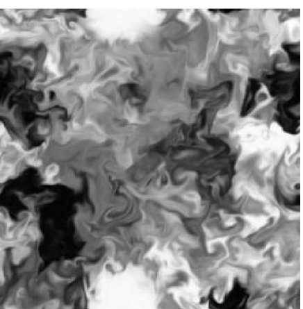
Figure 3: A view of the scalar field for a $256^{3}$ DNS. A recent injection can be seen, appearing as a white homogeneous zone.

Figure 4 shows several FDFs with extremely close means and variances. The cubes have been chosen so that $\overline{c}=0.5\pm 0.01$ and $\sigma_{s}^{2}=0.0055\pm 0.0001$.

Figure 4: Comparisons between a $\beta$ law (solid line) and several arbitrary chosen FDFs, of same mean ($\overline{c}=0.5\pm 0.01$) and variance ($\sigma_{s}^{2}=0.0055\pm 0.0001$)

5 FDF modelling

In the framework of LES, the FDF can be estimated either by solving an equation governing its evolution[23, 3] or by using a model for the FDF. The model proposed by Cook and Riley[5] uses a presumed form for the FDFs. It has drawn much attention and has been the subject of several studies[6, 24]. In this model, the main assumption is that the FDF can be approximated by a $\beta$ distribution with same mean and same variance as the real FDFs (i.e. the same first moments). The definition of the $\beta$ distribution is as follows:

$$\beta\left(x;\overline{c},\sigma_{s}^{2}\right)=\frac{x^{a-1}(1-x)^{b-1}}{B(a,b)},$$ (18)

with

$$B(a,b)=\frac{\Gamma(a)\,\Gamma(b)}{\Gamma(a+b)}=\int_{0}^{1}x^{a-1}(1-x)^{b-1}\,\mbox{d}x$$ (19)

$\Gamma(a)$ being the gamma function of Euler.

In order to have the right mean and variance, $a$ and $b$ must be chosen so that

$$a=\overline{c}\,\left(\frac{\overline{c}\,(1-\overline{c})}{\sigma_{s}^{2}}-1\right)~{}~{}~{}\mbox{and}~{}~{}~{}b=\frac{a}{\overline{c}}-a.$$

The presumed form for the FDF can be used in equation (13). This provides a model for $\overline{f(c)}$ whatever $f$ is, using $\overline{c}$ and $\sigma_{s}^{2}$ as variables. The estimator of $\overline{f(c)}$ can be written

$$\int f(x)\,\beta\left(x;\overline{c},\sigma_{s}^{2}\right)\,\mbox{d}x.$$ (20)

Since the definition of the variables is crucial for the optimal estimators, we will pay much attention to the often implicit choice of the fundamental variables. Here $\overline{c}$ and $\sigma_{s}^{2}$ are the variables. Hence we will denote $\pi_{1}=\left\{\overline{c},\sigma_{s}^{2}\right\}$ this first set of fundamental variables. The choice of $\beta$ distributions will be called the “$\beta$ assumption”.

The subgrid variance $\sigma_{s}^{2}$ cannot be computed using the large eddies $\overline{c}$ only. A sub-model is thus necessary so that the $\beta$ assumption can be used. Let us denote $\widehat{.}$ a test filter of a characteristic size twice as big as for $\overline{.}$. Cook and Riley assume that the subgrid variance is proportional to the quantity

$$\alpha=\widehat{\overline{c}^{2}}-\widehat{\overline{c}}^{2}.$$

This estimation is used to approximate the FDF and the whole model thus provides an estimation of $\overline{f(c)}$ based on the variables $\overline{c}$ and $\alpha$ only. We will denote $\pi_{2}=\left\{\overline{c},\alpha\right\}$ this second set of variables.

Another sub-model has been proposed by Pierce and Moin[25]. They assume that $\sigma_{s}^{2}$ is proportional to the modulus of the gradient of the filtered scalar, which we will denote $\epsilon_{\overline{c}}=(\partial_{i}\overline{c})^{2}$. In the following, we will denote $\pi_{2}=\left\{\overline{c},\epsilon_{\overline{c}}\right\}$ the variables corresponding to this modelization.

6 Validity of the $\beta$ assumption

Our purpose is to know if there is an optimal choice for the presumed form of the FDF. Of course this optimal choice depends on the variables $\pi$ used for the model. The fact that there is an optimal choice is not obvious. The optimal estimators used in the first part are defined in the case where a scalar quantity $\gamma$ has to be estimated using $\pi$. Here the model provides a function for each different value of $\pi$. No relevant measure of the error can be defined in this case. But we have the relation

$$\left.\left<\overline{f(c)}\right|\pi\right> = \left.\left<\int f(C)\,\mbox{d}_{s}(C)\,\mbox{d}C\right|\pi\right>$$ (21)

$$= \int f(C)~{}\left.\left<\mbox{d}_{s}(C)\right|\pi\right>~{}\mbox{d}C.$$ (22)

This means that $\left.\left<\mbox{d}_{s}\right|\pi\right>$ is the optimal estimator for the approximation of the FDF using $\pi$ since when it is used in equation (13), the estimator of $\overline{f(c)}$ which is obtained is the optimal estimator for $\overline{f(c)}$ using $\pi$. In this particular case the optimal estimator concept can therefore easily be extended. This quantity has already been considered in the case where the variables are $\overline{c}$ and $\sigma_{s}^{2}$. It has been called the conditional FDF[26]. It is sometimes refered to as the FPDF[27].

This optimal estimator can be computed using the following natural method: first, grid nodes are chosen for which $\pi$ has a value very close to an arbitrary given one, then the FDF is computed for each of these nodes, and finally, all the FDFs are averaged to obtain the optimal estimator.

Let us consider the set of variables $\pi_{1}=\left\{\overline{c},\sigma_{s}^{2}\right\}$, which is the case when the subgrid variance is known. Comparisons between beta distributions and the optimal estimators are shown for three sets of values of the variables in figure 5. The cubes which are selected for the computation of the optimal estimators are chosen so that $\overline{c}=0.5\pm 0.01$ and $\sigma_{s}^{2}=0.0055\pm 0.0001$ for the first comparison, $\overline{c}=0.25\pm 0.01$ and $\sigma_{s}^{2}=0.01\pm 0.001$ for the second one and $\overline{c}=0.1\pm 0.01$ and $\sigma_{s}^{2}=0.01\pm 0.001$ for the last one.

The correspondence between the $\beta$ distributions and the optimal estimators is excellent. The $\beta$ distributions can thus be considered as a very appropriate presumed form for the FDF, as long as $\sigma_{s}^{2}$ is known. We must point out that this does not mean that the FDFs are actually $\beta$ distributions[5], as shown figure 4. We agree [5] that the $\beta$ assumption seems to be appropriate for any subvolume. We think that a mathematical property of $\beta$ distributions could explain these results but we were not able to find it. Here, the size filter is about four grid nodes and has been chosen so that all values of $\overline{c}$, $\sigma_{s}^{2}$ (or $\alpha$) are well represented in the statistical sampling process.

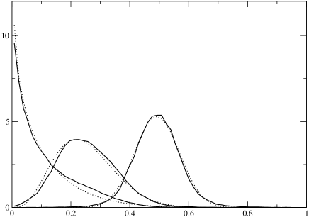
Figure 5: Comparisons between $\left.\left<\mbox{d}_{s}(C)\right|\overline{c},\sigma_{s}^{2}\right>$ and $\beta(C;\overline{c},\sigma_{s}^{2})$ for (i) $\overline{c}=0.5$ and $\sigma_{s}^{2}=0.0055$ (ii) $\overline{c}=0.25$ and $\sigma_{s}^{2}=0.01$ (iii) $\overline{c}=0.1$ and $\sigma_{s}^{2}=0.01$.

Let us consider the case when the variables of the model are $\overline{c}$ and $\alpha$. Figure 6 shows examples of FDFs for cubes which present the same values of $\overline{c}$ and $\alpha$. When compared to figure 4, it is observed that there are much larger differences between the FDFs. This is due to the fact that for given $\overline{c}$ and $\alpha$, different values of $\sigma_{s}^{2}$ are observed. This is what we will call the subgrid variance dispersion. For a given $\pi$ the subgrid variance dispersion can be quantified by the irreducible error made when estimating $\sigma_{s}^{2}$ using $\pi$. When for instance this error is small, the subgrid variance of cubes with very close $\pi$ values will be very close to $\left.\left<\sigma_{s}^{2}\right|\pi\right>$.

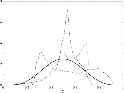
Figure 6: Comparisons between a $\beta$ law (solid line) and several arbitrary chosen FDFs, for $\overline{c}=0.5\pm 0.01$ and $\alpha=0.0125\pm 0.0005$.

Figure 7, the optimal estimators are compared to a $\beta$ distribution whose variance is $\left.\left<\sigma_{s}^{2}\right|\overline{c},\alpha\right>$ (the average of $\sigma_{s}^{2}$ for all the FDFs). The cubes which are selected for the computation of the optimal estimators are chosen so that $\overline{c}=0.5\pm 0.01$ and $\alpha=0.0125\pm 0.0005$ for the first case, $\overline{c}=0.355\pm 0.005$ and $\alpha=0.01\pm 0.001$ for the second case, and for the last one $\overline{c}=0.1\pm 0.01$ and $\alpha=0.001\pm 0.001$.

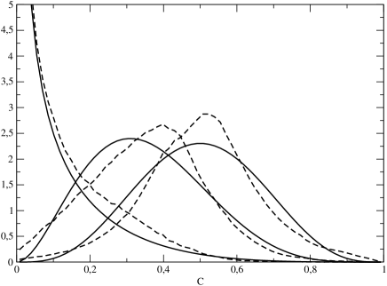
Figure 7: Comparisons between $\left.\left<\mbox{d}_{s}(C)\right|\overline{c},\alpha\right>$ and $\beta(C;\overline{c},\left.\left<\sigma_{s}^{2}\right|\overline{c},\alpha\right>)$

In this case, the $\beta$ distributions are not very close to the optimal estimators. This is due to the variance dispersion. This means that there is a better presumed form when $\alpha$ is used - closer to the optimal estimator. However, this form would be relevant for $\pi=\{\overline{c},\alpha\}$ only.

When choosing a set $\pi$ with less subgrid variance dispersion, the form of the optimal estimator must tend towards the form of the optimal estimator when $\sigma_{s}^{2}$ is known (when the dispersion is null). Hence, we conclude that the $\beta$ assumption is better when the subgrid variance dispersion is small.

Now that we have established that, when $\sigma_{s}^{2}$ is unknown, $\beta$ distributions are not as clearly appropriate as when the subgrid variance is known, the question is: is the error due to the difference between the optimal estimator of the FDF and the $\beta$ distribution a significant one ?

Using optimal estimators, it is possible to compute the supplementary error brought by the $\beta$ assumption alone for the estimation of $\overline{f(c)}$. This must be done for a given $f$.

Let us consider the following estimator for $\overline{f(c)}$ using $\pi$:

$$g_{f}(\pi)=\int f(C)~{}\beta\left(C;\overline{c},\left.\left<\sigma_{s}^{2}\right|\pi\right>\right)~{}\mbox{d}C.$$ (23)

It is obtained by replacing $\mbox{d}_{s}$ in (13) by a $\beta$ distribution. The variance of the $\beta$ distribution is the optimal estimator of $\sigma_{s}^{2}$ using $\pi$. The error made by this estimator can be compared to the irreducible error made by $\left.\left<\overline{f(c)}\right|\pi\right>$. The supplementary error made by the estimator (23) reflects the fact that $\beta$ distributions are not exactly the optimal estimators as shown figure 7 (or figure 5 even if the difference is slight).

We will now present results that have been obtained using histograms. All the quadratic errors have been normalized by the variance of the quantity which is estimated. This allows to compare two errors even if the quantity to estimate is not the same.

The results concerning the estimation of $\sigma_{s}^{2}$ are presented in table 1 concerning the estimation of $\sigma_{s}^{2}$. The irreducible error that is computed here reflects the subgrid variance dispersion. This dispersion is smaller when the variables are $\overline{c}$ and $\epsilon_{\overline{c}}$ than when the variables are $\overline{c}$ and $\alpha$.

Since the error brought by the $\beta$ assumption must be computed for a given $f$ we have chosen to do so for several $\beta$ distributions with different means and variances. This is a very plausible choice[25]. The comparison between the optimal estimators and the estimator $g_{f}(\pi)$ is presented in table 2. Column one is the error made by the optimal estimators, i.e. the irreducible error. Column two is the error made by $g_{f}(\pi)$, i.e. when using the $\beta$ assumption.

It can be observed that the supplementary error due to the $\beta$ assumption is always much smaller than the irreducible error. In most cases, it is one order of magnitude smaller. This confirms the previous results on the optimal estimators of the FDF.

The fact that the $\beta$ distributions are not very close to the optimal estimators of the FDFs has not a measurable incidence on the supplementary error. The latter can often be neglected and there is no need to search for a more relevant presumed form for the FDF.

Since the irreducible errors are normalized, they can be compared. The conclusion is that $\sigma_{s}^{2}$ is a quantity which is very difficult to estimate. The quantity $\overline{f(c)}$ is in general easier to estimate. In addition, the better $\sigma_{s}^{2}$ is estimated using a set of variables, the better the $\overline{f(c)}$ are estimated. For a few variables, the relative relevancy of a set does not depend on $f$.

Estimator	Normalized error
$\left.\left<\sigma_{s}^{2}\right|\overline{c},\epsilon_{\overline{c}}\right>$	0.215
$\left.\left<\sigma_{s}^{2}\right|\overline{c},\alpha\right>$	0.259
$\sigma_{s}^{2}=\kappa\,\alpha$	0.359

Table 1: Normalized quadratic errors for several optimal estimators of $\sigma_{s}^{2}$ (the optimal estimators are computed using the histogram technique). The constant $\kappa$ is chosen so that the error made by the Cook and Riley estimator of $\sigma_{s}^{2}$ is minimized.

Variables ($\pi$)	Error of $\left.\left<\overline{f(c)}\right|\pi\right>$	Error of $g_{f}(\pi)$
Mean 0.35, variance 0.01
$\overline{c}$, $\sigma_{s}^{2}$	0.043	0.051
$\overline{c}$,$\epsilon_{\overline{c}}$	0.095	0.099
$\overline{c}$,$\alpha$	0.136	0.140
Mean 0.15, variance 0.01
$\overline{c}$, $\sigma_{s}^{2}$	0.031	0.042
$\overline{c}$,$\epsilon_{\overline{c}}$	0.055	0.070
$\overline{c}$,$\alpha$	0.072	0.091
Mean 0.5, variance 0.01
$\overline{c}$, $\sigma_{s}^{2}$	0.041	0.063
$\overline{c}$,$\epsilon_{\overline{c}}$	0.092	0.107
$\overline{c}$,$\alpha$	0.130	0.146
Mean 0.5, variance 0.036
$\overline{c}$, $\sigma_{s}^{2}$	0.011	0.013
$\overline{c}$,$\epsilon_{\overline{c}}$	0.064	0.066
$\overline{c}$,$\alpha$	0.079	0.081

Table 2: Normalized quadratic errors of different estimators for the estimation of $\overline{f(c)}$. The mean and the variance of the different $f$ that have been chosen are specified.

7 Neural networks

As already underlined[5], the estimation of the subgrid variance $\sigma_{s}^{2}$ is the main problem in the presumed FDF approach. Rather complex models have been proposed[6] using dynamic approach and many new variables. Table 3 shows the irreducible error for different sets of variables computed using neural networks. One of these variables ($\overline{c}$) has often been neglected in the different models proposed. The results shown here suggest this is a mistake. On the contrary, the results show that the dissipation $\epsilon$ does not bring much information about $\sigma_{s}^{2}$.

Variables	Irreducible error
$\overline{c},\alpha$	0,259
$\overline{c},\epsilon_{\overline{c}}$	0,215
$\overline{c},\alpha,\epsilon_{\overline{c}}$	0,192
$\overline{c},\alpha,\epsilon$	0,258
$\alpha,\epsilon_{\overline{c}},\epsilon_{\widehat{\overline{c}}},\widehat{\epsilon_{\overline{c}}}$	0,173
$\overline{c},\alpha,\epsilon_{\overline{c}},\epsilon_{\widehat{\overline{c}}}$	0,158
$\overline{c},\alpha,\epsilon_{\overline{c}},\widehat{\epsilon_{\overline{c}}}$	0,152
$\overline{c},\alpha,\epsilon_{\overline{c}},\epsilon_{\widehat{\overline{c}}},\widehat{\epsilon_{\overline{c}}}$	0,137

Table 3: Irreducible error linked to different parameter sets. $64^{3}$ examples are used for evaluating the weights of the neural networks and $(128^{3}-64^{3})$ examples are used for estimating the irreducible error.

In addition, they show that the more variables are included in $\pi$, the better the estimation of the subgrid quantities - with errors much smaller than with usual models. Neural network can thus be considered as a new way towards optimal LES in the sense of Langford and Moser[1]. We think that they could be used directly for the modelling of unknown terms in LES and that they present some advantages: they do not need much data to estimate the conditional expectations correctly and they can reproduce highly non linear behaviours. It is possible to take physics directly into account when choosing the variables (galilean invariance[1], scale invariance or dimensional analysis arguments).

8 Conclusion

In agreement with Langford and Moser[1], we have used and explored the idea that in the framework of LES, once a set of variables has been chosen to estimate a given subgrid term, there is only one optimal estimator. Some of the properties of optimal estimators that are of interest for LES have been presented throughout this article. We have shown how optimal estimators could be computed using simple techniques if the number of variables is small, or neural networks if the number of variables is greater than 3.

As an illustration, the concept of optimal estimator was applied to the Cook and Riley subgrid model[5] for the scalar fluctuation, a model which is widely used and whose basis has already retained much attention in the literature. The concept of optimal estimator has been extended to the approximation of FDF and the main conclusion is that the $\beta$ assumption is very appropriate. When the error directly associated with the $\beta$ assumption for the estimation of a given quantity is compared with the irreducible error, it is found to be small. The largest error are associated with the estimation of the subgrid variance of the scalar fluctuations. That is the very point on which the Cook and Riley model needs to be improved.

In the paper we did not attempt to propose any new practical model for this scalar variance, but we used neural networks to see how closely the subgrid variance could be estimated. The error made by the optimal estimator is smaller when the number of relevant variables is increased.

The optimal estimation technique provides a way of assesssing which set of parameters will potentially lead to the most accurate subgrid model. It does not provide any information on how to specify the formulation of the model, but simply indicates if efforts for building a model with a given set of parameters are likely to be fruitful.

As the number of retained parameters is increased, it can become more and more difficult to propose a model formulation on the ground of physical reasoning, and this might suggest using the optimal estimator directly instead of a model. Then, neural networks would be used directly - instead of a modelization. This “NN guided LES” could constitute an optimal LES as defined by[1, 28]. We did not perform such a simulation in the present paper. This could be the subject of a future study (following the path explored by [28]).

This paper is an illustration of the relevance of optimal estimation techniques for the problem of subgrid modeling for LES. These techniques allow a thorough exploration of the behaviours of models in LES indicating the points which have to be improved in the models.

Appendix A Orthogonality relation

Let us give a short demonstration of (2). The quadratic error made by an estimator $g(\pi)$ can be developed:

$$\left<\left(\gamma-g(\pi)\right)^{2}\right> = \left<\left(\gamma-\left.\left<\gamma\right|\pi\right>\right)^{2}\right>+\left<\left(\left.\left<\gamma\right|\pi\right>-g(\pi)\right)^{2}\right>$$

$$+2\left<(\gamma-\left.\left<\gamma\right|\pi\right>)\,(\left.\left<\gamma\right|\pi\right>-g(\pi))\right>$$

Now, we have to show that the last term is null. It can be written

$$2\,\int(\gamma-\left.\left<\gamma\right|\pi\right>)\,(\left.\left<\gamma\right|\pi\right>-g(\pi))\,p(\gamma,\pi)\,\mbox{d}\gamma\,\mbox{d}\pi$$

$$= 2\,\int(\left.\left<\gamma\right|\pi\right>-g(\pi))\,p(\pi)\left(\int(\gamma-\left.\left<\gamma\right|\pi\right>)\,p(\gamma|\pi)\,\mbox{d}\gamma\right)\,\mbox{d}\pi$$

Since $\left.\left<\gamma\right|\pi\right>=\int\gamma p(\gamma|\pi)\,\mbox{d}\gamma$, the previous quantity is null and the orthogonality relation holds.

Appendix B Successive conditioning

Let $g(\pi)$ be an estimator of $\gamma$ using $\pi$. We will note $p(g(\pi)=g)$ or $p(g)$ the PDF that $g(\pi)=g$. Then we have

$$\left.\left<\gamma\right|g(\pi)=g\right>\,p(g(\pi)=g) = \int\gamma\,p(\gamma,g)\,\mbox{d}\gamma$$

$$= \int\gamma\,p(\gamma,\pi,g)\,\mbox{d}\gamma\,\mbox{d}\pi$$

$$= \int\gamma\,p(\gamma,\pi)\,\delta(g(\pi)-g)\,\mbox{d}\gamma\,\mbox{d}\pi$$

$$= \int\left(\int\gamma\,p(\gamma|\pi)\,\mbox{d}\gamma\right)\,p(\pi)\,\delta(g(\pi)-g)\,\mbox{d}\pi$$

$$= \int\left.\left<\gamma\right|\pi\right>\,p(\pi)\,\delta(g(\pi)-g)\,\mbox{d}\pi.$$

And if $g(\pi)=\left.\left<\gamma\right|\pi\right>$ then

$$\left.\left<\gamma\right|\left.\left<\gamma\right|\pi\right>=g\right>\,p(g) = \int\left.\left<\gamma\right|\pi\right>\,p(\pi)\,\delta(\left.\left<\gamma\right|\pi\right>-g)\,\mbox{d}\pi$$

$$= g\,\int p(\pi)\,\delta(\left.\left<\gamma\right|\pi\right>-g)\,\mbox{d}\pi$$

$$= g\int p(\pi,g)\,\mbox{d}\pi$$

$$= g\,p(g)$$

Hence, $\left.\left<\gamma\right|g(\pi)=g\right>=g$, which can be written

$$\left.\left<\gamma\right|\left.\left<\gamma\right|\pi\right>\right>=\left.\left<\gamma\right|\pi\right>.$$

Appendix C Filtering

The filtering can be written

$$\overline{c}(\vec{r})=\int G(\vec{r}-\vec{x})\,c(\vec{x})\,\mbox{d}\vec{x}$$

or $\overline{c}=G*c$. Let us assume that we have $0\leq c\leq 1$ and that we want

$$0\leq\overline{c}\leq 1.$$ (24)

If $G(\vec{x})\geq 0\;\forall\vec{x}$ we can write

$$0\leq\overline{c}\leq\overline{1}.$$

If $G$ is not positive, the inequality can be false. Thus it is necessary that $G$ should be positive. In order to have (24) verified, $G$ must have the property $\overline{1}=1$, which can be written $\int G=1$.

Let us now define $V_{D}(C)=\overline{H(C-c(\vec{x}))}$. The physical meaning of this quantity is not as clear as in the case of the box filter. Anyway, the FDF is still the derivative of $V_{D}$. We can write

$$V_{D}(a)-V_{D}(b)=\overline{H(a-c)-H(b-c)}.$$

If $a\geq b$ then $H(a-c(\vec{x})-H(b-c(\vec{x}))\geq 0$. If the filter is positive, then $V_{D}(a)\geq V_{D}(b)$ and $V_{D}$ is a growing function. If $G$ is not positive, this is not granted. Since the FDF is the derivative of $V_{D}$, it is positive only if the filter is positive. Finally, we have $V_{D}(1)=\overline{1}=\int\mbox{d}_{s}$, so that the FDF is normalized only if $\int G=1$.

The filters are generally chosen so that $\int G=1$. The previous arguments show that they should be chosen positive, too. The box filter has been chosen for historical[5, 6] and clarity reasons. But it is an invertible filter, whereas the filters that should be considered in the framework of LES should be non-invertible[1]. All the non-invertible filters that have been proposed are not positive. We propose here a new filter that could be more relevant. It is defined by

$$G(\vec{x})=\prod_{i=1}^{3}\frac{2}{\pi\,\ell}\;\mbox{sinc}^{2}\frac{x}{\ell}.$$ (25)

This filter is non-invertible (since the Fourier Transform of $\mbox{sinc}^{2}$ is a triangle function), normalized and positive. We think that the choice of a particular filter has not much importance while the error made by the estimators is large. For very small errors, a difference could probably be found between the error made by the estimators when using an invertible filter and the error when using a non-invertible filter. This could probably be seen using neural networks when computing the irreducible error.

References

- [1] J.A. Langford and R.D. Moser, “Optimal LES formulations for isotropic turbulence”, J. Fluid Mech. 398, 321 (1999).
- [2] U. Schumann, “Subgrid scale model for finite difference simulations of turbulent flows in plane channels and annuli”, J. of Comp. Phys., 18, 376 (1975).
- [3] P.J. Colucci, F.A. Jaberi, P. Givi, and S.B. Pope, “Filtered density function for large eddy simulation of turbulent reacting flows”, Phys. Fluids 10, 499 (1998).
- [4] J.P. Bertoglio, A stochastic subgrid model for sheared turbulence. Macroscopic modelling of turbulent flows, Lecture Notes in Physics, Berlin and New York, Springer-Verlag, p. 100-119 (1985).
- [5] A.W. Cook, J.J. Riley, “A subgrid model for equilibrium chemistry in turbulent flows”, Phys. Fluids 6, 2868 (1994).
- [6] C. Wall, B.J. Boersma, and P. Moin. “An evaluation of the assumed beta probability density function subgrid-scale model for large eddy simulation of nonpremixed turbulent combustion with heat release”, Phys. Fluids, 12, 2522 (2000).
- [7] R. Deutsch, Estimation theory (Prentice Hall, 1965).
- [8] L. Gorden and R. Olshen, “Asymptotically efficient solutions to the classification problem”, Ann. Statist. 6, 515 (1978).
- [9] C. Stone, “Consistent nonparametric regression”, Ann. of Statit. 8, 1348 (1977).
- [10] I. Steinwart, “Consistency of support vector machines and other regularized kernel classifiers” Information Theory, IEEE Trans. 51, 128 (2005).
- [11] V.N. Vapnik and A.Ya. Chervonenkis, Theory of Pattern Recognition (in Russian) (Nauka, Moscow, 1974).
- [12] C.M. Bishop. Neural Networks for Pattern Recognition. (Oxford University Press, 1995).
- [13] H. White, “Connectionist Nonparametric Regression: Multilayer Feedforward Networks Can Learn Arbitrary Mappings”, Neural Networks 3, 535 (1990).
- [14] D. Rumelhart, G. Hinton, and R. Williams, “Learning internal representations by error propagation”, Neurocomputing, J. Anderson and E. Rosenfeld eds., 675-695. Cambridge (MA), MIT Press (1988).
- [15] S. Haykin and J. Principle, “Using Neural Networks to Dynamically model Chaotic events such as sea clutter; making sense of a complex world”, IEEE Signal Processing Magazine 66, 81 (1998).
- [16] J.-M. Friedt, O. Teytaud and M. Planat, “Learning from Noise in Chua’s Oscillator”, Proceedings of the 16th International Conference on Noise in Physical Systems and 1/f Fluctuations, pp 491-496 (2001).
- [17] C. Lee, J. Kim, and D. Babcok, “Application of neural networks for turbulence control for drag reduction”, Phys. Fluids 9, 1740 (1997).
- [18] S. Mukherjee, E. Osuna, F. Girosi, “Nonlinear prediction of chaotic time series using support vector machines”, in Proc.of IEEE NNSP 97, Amelia Island, FL, 511-519 (1997).
- [19] H. Ali and Y. Najjar, “Neuronet - Based Approach for Assessing the Liquefaction Potential of Soils”, Transportation Research Records, No. 1633, pp. 3 -8 (1999).
- [20] J.A.K. Suykens, T. Van Gestel, J. De Brabanter, B. De Moor and J. Vandewalle, Least Squares Support Vector Machines (World Scientific, Singapore, 2002).
- [21] S.B. Pope, “Pdf methods for turbulent reactive flows”, Prog. Energy Combust. Sci. 11 119 (1985).
- [22] M. Elmo, A. Moreau, J.P. Bertoglio, V.A. Sabel’nikov, “Mixing in isotropic turbulence with scalar injection and applications to subgrid modeling”, Flow, Turb. Combust. 65 113 (2000).
- [23] F. Gao and E.E. O’Brien, “A large-eddy simulation scheme for turbulent reacting flows”, Phys. Fluids A, 5,1282 (1993).
- [24] J. Jimenez, A. Liñan, M.M. Rogers, and F.J. Higuera, “A priori testing of subgrid models for chemically reacting non-premixed turbulent shear flows”, J. Fluid Mech 349, 149 (1997).
- [25] C.D. Pierce and P. Moin, “A dynamic model for subgrid-scale variance and dissipation rate of a conserved scalar”, Phys. Fluids 10,3041 (1998).
- [26] C. Tong, “Measurements of conserved scalar filtered density function in a turbulent jet”, Phys. Fluids 13,2923 (2001).
- [27] H. Pitsch, “Large-Eddy Simulation of Turbulent Combustion”, Annu. Rev. Fluid Mech. 38,453 (2006).
- [28] S. Völker, R.D. Moser and P. Venugopal, “Optimal large eddy simulation of turbulent channel flow based on direct numerical simulation statistical data”, Phys. Fluids 14,3675 (2002).