Brewster angle for anisotropic materials from the extinction theorem

Abstract

We explore the physical origin of Brewster angle in the external and internal reflections associated with an anisotropic material. We obtain the expressions of the reflected fields and the existence condition of Brewster angle by using the extinction theorem. It is found that the Brewster angle will occur if the total contribution of the anisotropic material’s electric and magnetic dipoles to the reflection field becomes zero. In internal reflection, the requirements on the material parameters ${\bm{\varepsilon}}$ and ${\bm{\mu}}$ for Brewster angle are the same as those in external reflection, and the Brewster angle is just the refraction angle in external reflection at the incidence of external Brewster angle. In contrast to the conventional isotropic medium, an anisotropic material can exhibit Brewster angle for both TE and TM waves due to its anisotropy. The results of the present paper are applicable to anisotropic dielectric and magnetic materials, including metamaterials.

I Introduction

As well known, Brewster angle is the angle of incidence at which the incident light is reflected without the polarization component parallel to the plane of incidence. At the Brewster angle, the reflected light is perpendicular to the refracted light. The physics accounting for such a phenomenon is that the vibration of electrons in the second medium can not generate the reflected light which travels perpendicular to the transmitted light Born . These conclusions only hold for isotropic dielectric materials. Since conventional transparent isotropic materials can be regarded nonmagnetic, these conclusions are applicable to them.

However, the advent of a new kind of artificial materials, named as left-handed materials, changes the situation. The left-handed material was hypothesized by Veselago Veselago1968 and can exhibit many exotic electromagnetic properties, among which the most well known is the negative refraction. Since the negative refraction was experimentally observed in a structured metamaterial composed of arrays of conducting split ring resonators (SRRs) and wires Shelby2001 , the left-handed material has sparked great interest Pendry2000 ; Lindell2001 ; Smith2003 ; Smith2004 ; Hu2002 ; Luo2002 ; Belov2003 ; Lakhtakia2004 ; Lakhtakia2006 ; Luo2005 ; Luo2006 . Metamaterials have been explored to exhibit Brewster angle not only for TM (traverse magnetic) waves, but also for TE (traverse electric) waves Zhou2003 ; Grzegorczyk2005 . Then, one enquires naturally: How on earth do TE waves exhibit Brewster angle in metamaterials? Whether the mechanism of Brewster angle for TE waves is the same as that for TM waves, i.e., just described above?

It is well accepted that the molecular optics theory can give much deeper physical insight into the interaction of electromagnetic wave with material than do Maxwell theory Feynman1963 ; Wolf1972 ; Reali1982 ; Karam1997 ; Doyle1985 . But such an approach is less frequently employed because it involves integral-differential equations difficult to solve. Recently, Lai et al. Lai2002 used the method of superposition of retarded field to discuss the reflection and refraction law of electromagnetic wave incident on an isotropic medium. Along that way, Fu et al. Fu2005 explored the Brewster condition for light incident from the vacuum onto an isotropic material with negative index. Since the metamaterials are actually anisotropic, it is necessary to generalize the Brewster condition from the isotropic material to the anisotropic material. At the same time, in most work dealing with the interaction of electromagnetic wave with material by the molecular optics theory, often considered is the wave incident from the vacuum into a dielectric material Feynman1963 ; Reali1982 ; Karam1996 , but the case of wave incident from the vacuum on a magnetic material, or from a material into vacuum is rarely investigated.

The purpose of this paper is to present a detailed investigation on the mechanism of Brewster angle in external and internal reflections associated with an anisotropic dielectric-magnetic material. We use the extinction theorem of the molecular optics to derive the reflected fields and the existence condition of Brewster angle. We find that Brewster angle will occur if the contributions of the electric and magnetic dipoles to the reflected field add up to zero. We also study in detail the impacts of the material parameters ${\bm{\varepsilon}}$ and ${\bm{\mu}}$ on the Brewster angle. The results extend the conclusions about Brewster angle in isotropic materials Fu2005 ; Lai2002 ; Reali1982 ; Doyle1985 and can provide references in manufacturing materials for specific purposes, such as making polarization devices. The conclusions also provide a new and deep look on those obtained by Maxwell theory Shen2006 .

II Brewster angle in external reflection

In molecular optics theory, a bulk material can be regarded as a collection of molecules (or atoms) embedded in the vacuum. Under the action of an incident field, the molecules oscillate as electric and magnetic dipoles and emit radiations. The radiation field and the incident field interact to form the new transmitted field in the material and the reflection field outside the material Born .

In this section, we first employ the Ewald-Oseen extinction theorem to deduce the expressions of radiated fields generated by dipoles in the external reflection of waves incident on an anisotropic dielectric-magnetic material. Then we study the Brewster angle condition and discuss the results.

II.1 Extinction theorem and external reflection

Let a monochromatic electromagnetic field of ${\bf E}_{i}={\bf E}_{i0}\exp{(i{\bf k}_{i}\cdot{\bf r}-i\omega t)}$ and ${\bf H}_{i}={\bf H}_{i0}\exp{(i{\bf k}_{i}\cdot{\bf r}-i\omega t)}$ incident from the vacuum on an anisotropic material filling the semi-infinite space $z>0$ with ${\bf k}_{i}=k_{ix}\hat{{\bf x}}-k_{iz}\hat{{\bf z}}$. The $x-z$ plane is the plane of incidence and the schematic diagram is shown in Fig. 1. Since the material responds linearly, all the fields have the same dependence of $\exp{(-i\omega t)}$ which will be omitted subsequently for simplicity. We assume that the reflected fields are ${\bf E}_{r}={\bf E}_{r0}\exp{(i{\bf k}_{r}\cdot{\bf r})}$ and ${\bf H}_{r}={\bf H}_{r0}\exp{(i{\bf k}_{r}\cdot{\bf r})}$, and the transmitted fields are ${\bf E}_{t}={\bf E}_{t0}\exp{(i{\bf k}_{t}\cdot{\bf r})}$ and ${\bf H}_{t}={\bf H}_{t0}\exp{(i{\bf k}_{t}\cdot{\bf r})}$, where ${\bf k}_{r}=k_{rx}\hat{{\bf x}}-k_{rz}\hat{{\bf z}}$ and ${\bf k}_{t}=k_{tx}\hat{{\bf x}}+k_{tz}\hat{{\bf z}}$. The permittivity and permeability tensors of the anisotropic material are simultaneously diagonal in the principal coordinate system, $\bm{\varepsilon}=\hbox{diag}[\varepsilon_{x},\varepsilon_{y},\varepsilon_{z}],~{}~{}\bm{\mu}=\hbox{diag}[\mu_{x},\mu_{y},\mu_{z}]$.

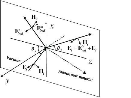
Figure 1: Schematic diagram for how the reflected and transmitted fields of TE waves are generated by the incident field and radiated fields of dipoles. In the vacuum, the reflected field ${\bf E}_{r}={\bf E}^{e}_{r0}+{\bf E}^{m}_{r0}$, while the transmitted field ${\bf E}_{t}={\bf E}_{i}+{\bf E}^{in}_{rad}$ in the material. When ${\bf E}^{e}_{r0}+{\bf E}^{m}_{r0}=0$, ${\bf E}_{r0}=0$ and Brewster angle occurs for TE waves. The dotted line is the transmitted wave in negative refraction.

Inside the anisotropic material, the incident field drive the dipoles to oscillate and radiate. The electric fields radiated by electric dipoles and magnetic dipoles are respectively decided by Born

$${\bf E}^{e}_{rad}=\nabla(\nabla\cdot{\bf{\Pi}}_{e})-\varepsilon_{0}\mu_{0}\frac{\partial^{2}{\bf{\Pi}}_{e}}{\partial t^{2}},$$ (1)

$${\bf E}^{m}_{rad}=-\mu_{0}\nabla\times\frac{\partial{\bf{\Pi}}_{m}}{\partial t}.$$ (2)

And the magnetic fields generated by magnetic dipoles and electric dipoles are

$${\bf H}^{m}_{rad}=\nabla(\nabla\cdot{\bf{\Pi}}_{m})-\varepsilon_{0}\mu_{0}\frac{\partial^{2}{\bf{\Pi}}_{m}}{\partial t^{2}},$$ (3)

$${\bf H}^{e}_{rad}=\varepsilon_{0}\nabla\times\frac{\partial{\bf{\Pi}}_{e}}{\partial t}.$$ (4)

Here ${\bf\Pi}_{e}$ and ${\bf\Pi}_{m}$ are the Hertz vectors,

$${\bf\Pi}_{e}({\bf r})=\int\frac{{\bf P}({\bf r^{\prime}})}{\varepsilon_{0}}G({\bf r}-{\bf r}^{\prime})\hbox{d}{\bf r}^{\prime},$$ (5)

$${\bf\Pi}_{m}({\bf r})=\int{\bf M}({\bf r^{\prime}})G({\bf r}-{\bf r}^{\prime})\hbox{d}{\bf r}^{\prime}.$$ (6)

${\bf P}$ is the dipole moment density of electric dipoles and ${\bf M}$ is that of magnetic dipoles, which are related to the transmitted fields by ${\bf P}=\varepsilon_{0}\bm{\chi}_{e}\cdot{\bf E}_{t}$ and ${\bf M}=\bm{\chi}_{m}\cdot{\bf H}_{t}$, where the electric susceptibility $\bm{\chi}_{e}=(\bm{\varepsilon}/{\varepsilon_{0}})-1$ and the magnetic susceptibility $\bm{\chi}_{m}=(\bm{\mu}/{\mu_{0}})-1$. The Green function is $G({\bf r}-{\bf r}^{\prime})=\exp{(ik_{i}|{\bf r}-{\bf r}^{\prime}|)}/(4\pi|{\bf r}-{\bf r}^{\prime}|)$. To evaluate the Hertz vectors, we firstly represent the Green function in the Fourier form. Then, inserting it into Eqs. (5) and (6) and using the delta function definition and contour integration method Reali1982 , the Hertz vectors can be evaluated as

$${\bf\Pi}_{e}=\left\{\begin{array}[]{cc}\displaystyle-\frac{\bm{\chi}_{e}\cdot{\bf E}_{t0}\exp{(ik_{tx}x-ik_{1z}z})}{2k_{1z}(k_{1z}+k_{tz})},&-\infty<z<0\\ \displaystyle\frac{\bm{\chi}_{e}\cdot{\bf E}_{t0}\exp{(i{\bf k}_{1}\cdot{\bf r})}}{2k_{1z}(k_{1z}-k_{tz})}+\frac{\bm{\chi}_{e}\cdot{\bf E}_{t0}\exp{(i{\bf k}_{t}\cdot{\bf r})}}{k_{t}^{2}-k_{i}^{2}},&0\leq z<\infty\end{array}\right.$$ (7)

$${\bf\Pi}_{m}=\left\{\begin{array}[]{cc}\displaystyle-\frac{\bm{\chi}_{m}\cdot{\bf H}_{t0}\exp{(ik_{tx}x-ik_{1z}z)}}{2k_{1z}(k_{1z}+k_{tz})},&-\infty<z<0\\ \displaystyle\frac{\bm{\chi}_{m}\cdot{\bf H}_{t0}\exp{(i{\bf k}_{1}\cdot{\bf r})}}{2k_{1z}(k_{1z}-k_{tz})}+\frac{\bm{\chi}_{m}\cdot{\bf H}_{t0}\exp{(i{\bf k}_{t}\cdot{\bf r})}}{k_{t}^{2}-k_{i}^{2}},&0\leq z<\infty\end{array}\right.$$ (8)

where ${\bf k}_{1}=k_{tx}\hat{{\bf x}}+k_{1z}\hat{{\bf z}}$, $k_{1z}^{2}=k_{i}^{2}-k_{tx}^{2}$, and we have used the Faraday’s law ${\bf H}_{t}=({\bf k}_{t}\times{\bf E}_{t})/(\omega{\bm{\mu}})$ which can also be established by the molecular theory.

Following the extinction theorem, the incident field is extinguished inside the material and is replaced by the transmitted field Born . Then, we get

$${\bf E}_{t}={\bf E}^{e}_{rad}+{\bf E}^{m}_{rad}+{\bf E}_{i}.$$ (9)

Using Eqs. (7) and (8) and inserting Eqs. (1) and (2) into Eq. (9), we come to the following conclusions.

(1). Comparing terms of the phase factor $\exp{(i{\bf k}_{1}\cdot{\bf r})}$ in Eq. (9), we know that ${\bf k}_{1}={\bf k}_{i}$ and $k_{ix}=k_{tx}$. This is just the Snell’s law: $k_{i}\sin\theta_{i}=k_{t}\sin\theta_{t}$.

(2). At the same time, the incident field can be written in terms of the transmitted field

$${\bf E}_{i0}=\frac{{\bf k}_{i}\times[{\bf k}_{i}\times(\bm{\chi}_{e}\cdot{\bf E}_{t0})]}{2k_{iz}(k_{iz}-k_{tz})}+\frac{{\bf k}_{i}\times\{\bm{\chi}_{m}\cdot[{\mu_{0}}{\bm{\mu}}^{-1}\cdot({\bf k}_{t}\times{\bf E}_{t0})]\}}{2k_{iz}(k_{iz}-k_{tz})}.$$ (10)

Equation (10) is actually the expression of the Ewald-Odseen extinction theorem. It shows quantitatively how the radiation field of dipoles extinguish the incident field.

(3). The terms with the phase factor $\exp{(i{\bf k}_{t}\cdot{\bf r})}$ in Eq. (9) yields the dispersion relation

$$\frac{k_{tx}^{2}}{\mu_{z}\varepsilon_{y}}+\frac{k_{tz}^{2}}{\mu_{x}\varepsilon_{y}}=\omega^{2}$$ (11)

for TE waves. In order to guarantee $k_{tz}$ real, it requires that $\varepsilon_{y}{\mu_{z}}<\varepsilon_{0}{\mu_{0}}\cap{\mu_{x}}{\mu_{z}}<0$, or $\varepsilon_{y}{\mu_{z}}>0\cap{\mu_{x}}{\mu_{z}}>0$. In addition, there will exist a critical angle of incidence $\theta^{TE}_{C}=\sin^{-1}\sqrt{{\mu_{z}}\varepsilon_{y}/{\varepsilon_{0}}\mu_{0}}$ if $0<{\mu_{z}}\varepsilon_{y}<{\varepsilon_{0}}\mu_{0}$. Outside the anisotropic material, the contributions from the electric and magnetic dipoles form the reflected field ${\bf E}_{r}$. Applying Eqs. (7) and (8) for $z<0$ to Eqs. (1) and (2), we obtain

$${\bf E}_{r0} = {\bf E}^{e}_{r0}+{\bf E}^{m}_{r0}$$ (12)

$$= \frac{{\bf k}_{r}\times[{\bf k}_{r}\times(\bm{\chi}_{e}\cdot{\bf E}_{t0})]}{2k_{iz}(k_{iz}+k_{tz})}+\frac{{\bf k}_{r}\times\{\bm{\chi}_{m}\cdot[{\mu_{0}}{\bm{\mu}}^{-1}\cdot({\bf k}_{t}\times{\bf E}_{t0})]\}}{2k_{iz}(k_{iz}+k_{tz})}.$$

where ${\bf k}_{r}=k_{ix}\hat{{\bf x}}-k_{iz}\hat{{\bf z}}$. Equations (10) and (12) hold for both TE and TM waves. And we obtain the reflection coefficient $R_{E}(={E}_{r0}/{E}_{i0})$ and the transmission coefficient $T_{E}(={E}_{t0}/{E}_{i0})$ for TE waves

$$R_{E}=\frac{\mu_{x}k_{iz}-\mu_{0}k_{tz}}{\mu_{x}k_{iz}+\mu_{0}k_{tz}},~{}~{}~{}T_{E}=\frac{2\mu_{x}k_{iz}}{\mu_{x}k_{iz}+\mu_{0}k_{tz}}.$$ (13)

Analogously, we can derive the incident magnetic field

$${\bf H}_{i0}=\frac{{\bf k}_{i}\times[{\bf k}_{i}\times(\bm{\chi}_{m}\cdot{\bf H}_{t0})]}{2k_{iz}(k_{iz}-k_{tz})}+\frac{{\bf k}_{i}\times\{\bm{\chi}_{e}\cdot[{\varepsilon_{0}}{\bm{\varepsilon}}^{-1}\cdot({\bf k}_{t}\times{\bf H}_{t0})]\}}{2k_{iz}(k_{iz}-k_{tz})},$$ (14)

the reflected magnetic field

$${\bf H}_{r0} = {\bf H}^{m}_{r0}+{\bf H}^{e}_{r0}$$ (15)

$$= \frac{{\bf k}_{r}\times[{\bf k}_{r}\times(\bm{\chi}_{m}\cdot{\bf H}_{t0})]}{2k_{iz}(k_{iz}+k_{tz})}+\frac{{\bf k}_{r}\times\{\bm{\chi}_{e}\cdot[{\varepsilon_{0}}{\bm{\varepsilon}}^{-1}\cdot({\bf k}_{t}\times{\bf H}_{t0})]\}}{2k_{iz}(k_{iz}+k_{tz})},$$

and the dispersion relation

$$\frac{k_{tx}^{2}}{\varepsilon_{z}\mu_{y}}+\frac{k_{tz}^{2}}{\varepsilon_{x}\mu_{y}}=\omega^{2}$$ (16)

for TM waves. To ensure $k_{tz}$ real, it needs that $\varepsilon_{z}{\mu_{y}}<\varepsilon_{0}{\mu_{0}}\cap{\varepsilon_{x}}{\varepsilon_{z}}<0$, or $\varepsilon_{z}{\mu_{y}}>0\cap{\varepsilon_{x}}{\varepsilon_{z}}>0$. In addition, there will be a critical angle of incidence $\theta^{TM}_{C}=\sin^{-1}\sqrt{{\mu_{y}}\varepsilon_{z}/{\varepsilon_{0}}\mu_{0}}$ if $0<{\mu_{y}}\varepsilon_{z}<{\varepsilon_{0}}\mu_{0}$. And we obtain the reflection coefficient $R_{H}(={H}_{r0}/{H}_{i0})$ and the transmission coefficient $T_{H}(={H}_{t0}/{H}_{i0})$ for TM waves as

$$R_{H}=\frac{\varepsilon_{x}k_{iz}-\varepsilon_{0}k_{tz}}{\varepsilon_{x}k_{iz}+\varepsilon_{0}k_{tz}},~{}~{}~{}T_{H}=\frac{2\varepsilon_{x}k_{iz}}{\varepsilon_{x}k_{iz}+\varepsilon_{0}k_{tz}},$$ (17)

respectively.

Obviously, Eqs. (13) and (17) are in agreement with the results obtained by the formal approach of Maxwell’s equations. At the same time, we can see that the extinction theorem plays the role of the boundary conditions in Maxwell approach.

II.2 The origin of Brewster angle and the impact of $\bm{\varepsilon}$ and $\bm{\mu}$

Let us now apply the results just obtained to study the origin of Brewster angle in the reflection of waves incident on the anisotropic material.

If the power reflectivity $r=|R|^{2}=0$, there is no reflected wave and the incident angle is named as Brewster angle Kong2000 . Now we discuss TE and TM waves separately. In order to meet $r_{E}=|{\bf E}_{r0}/{\bf E}_{i0}|^{2}=0$, it requires that ${\bf E}_{r0}=0$ in Eq. (12), i.e.,

$$\frac{(1-{\varepsilon_{y}}/{\varepsilon_{0}})k_{i}^{2}-k_{ix}k_{tx}(1-{\mu_{0}}/{\mu_{z}})+k_{iz}k_{tz}(1-{\mu_{0}}/{\mu_{x}})}{2k_{iz}(k_{iz}+k_{tz})}=0.$$ (18)

From Eq. (18), it follows that if

$$0<\frac{1-\frac{\mu_{0}\varepsilon_{y}}{\mu_{x}\varepsilon_{0}}}{1-\frac{\mu_{0}\mu_{0}}{\mu_{x}\mu_{z}}}<1$$ (19)

the Brewster angle for TE waves is

$$\theta_{B}^{TE}=\sin^{-1}\sqrt{\frac{1-\frac{\mu_{0}\varepsilon_{y}}{\mu_{x}\varepsilon_{0}}}{1-\frac{\mu_{0}\mu_{0}}{\mu_{x}\mu_{z}}}}.$$ (20)

To realize $r_{H}=|{\bf H}_{r0}/{\bf H}_{i0}|^{2}=0$, it is needed that ${\bf H}_{r0}=0$, that is,

$$\frac{(1-{\mu_{y}}/{\mu_{0}})k_{i}^{2}-k_{ix}k_{tx}(1-{\varepsilon_{0}}/{\varepsilon_{z}})+k_{iz}k_{tz}(1-{\varepsilon_{0}}/{\varepsilon_{x}})}{2k_{iz}(k_{iz}+k_{tz})}=0.$$ (21)

Similarly, we conclude that under the condition

$$0<\frac{1-\frac{\varepsilon_{0}\mu_{y}}{\varepsilon_{x}\mu_{0}}}{1-\frac{\varepsilon_{0}\varepsilon_{0}}{\varepsilon_{x}\varepsilon_{z}}}<1,$$ (22)

there exists a Brewster angle for TM waves

$$\theta_{B}^{TM}=\sin^{-1}\sqrt{\frac{1-\frac{\varepsilon_{0}\mu_{y}}{\varepsilon_{x}\mu_{0}}}{1-\frac{\varepsilon_{0}\varepsilon_{0}}{\varepsilon_{x}\varepsilon_{z}}}}.$$ (23)

We find that the Brewster condition of TE waves is only related to three components of the material parameters ${\bm{\varepsilon}}$ and ${\bm{\mu}}$, while that of TM waves depends on the other three components. Therefore, we can let the anisotropic material exhibit Brewster angles for TE, or TM, or both waves through choosing appropriate ${\bm{\varepsilon}}$ and ${\bm{\mu}}$. This is in sharp contrast with the regular isotropic material case where only one of TE and TM waves can exhibit Brewster angle.

There are different sign combination of ${\bm{\varepsilon}}$ and ${\bm{\mu}}$ for the anisotropic materials. According to the form of dispersion relation Smith et al. classify the anisotropic material into three types : cutoff, never cutoff, and anti-cutoff Smith2003 . We give an example of the reflectivity for wave incident into each type in Fig. 2.

Figure 2: Reflectivity $r$ of TE waves as a function of the incidence angle $\theta_{i}$ at the interface between vacuum and an cutoff, never cutoff, and anti-cutoff anisotropic materials. There exists a Brewster angle for the three cases. Note that there exists a critical angle of incidence $\theta^{TE}_{C}$ in reflection on anti-cutoff anisotropic material.

Clearly, we see that there is Brewster angle in the reflection of TE (the case of TM waves can be discussed similarly). To explain the Brewster condition vividly, we illustrate in Figs. 3, 4 and 5 the magnitudes of radiation fields for the examples in Fig. 2. It is clear that when the total radiated field of electric and magnetic dipoles is zero, i.e., ${\bf E}_{r0}^{e}+{\bf E}_{r0}^{m}=0$, the Brewster angle occurs. Each of the three classes of media has two subtypes: one positive (fig(a))and one negative (fig(b)) refracting. Comparing the two subtypes of each figure, one can find that the reflectivity is the same, but the field magnitudes ${\bf E}^{e}_{r0}$ and ${\bf E}^{m}_{r0}$ are totally different because signs of ${\bm{\varepsilon}}$ and ${\bm{\mu}}$ are reversed. Even if one element’s sign changes, such as $\mu_{z}$ in Figs. 3(b) and 4(b), ${\bf E}^{e}_{r0}$ and ${\bf E}^{m}_{r0}$ alter accordingly. If one element’s magnitude and sign change, then not only the magnitude but also the phase of the radiated field can change, such as in Figs. 4(b) and 5(b).

Figure 3: Reflected field magnitudes, normalized by the corresponding incident field magnitudes, for TE wave incident from vacuum into a cutoff anisotropic material. Since $\varepsilon_{y}=\varepsilon_{0}$, the radiated electric fields of electric dipoles ${\bf E}^{e}_{r0}=0$, then ${\bf E}_{r0}={\bf E}^{m}_{r0}$. When ${\bf E}^{m}_{r0}=0$ Brewster angle $\theta_{B}^{TE}$ appears, as shown in (a).

Figure 4: Reflected field magnitudes, normalized by the corresponding incident field magnitudes, for TE wave incident from vacuum into a never cutoff anisotropic material.

Figure 5: Reflected field magnitudes, normalized by the corresponding incident field magnitudes, for TE wave incident from vacuum into an anti-cutoff anisotropic material. There exist a critical angle $\theta^{TE}_{C}$ for incidence and $\theta^{TE}_{C}>\theta^{TE}_{B3}$, which is called as the inversion of critical angle.

In the next step, we study the impacts of ${\bm{\varepsilon}}$ and ${\bm{\mu}}$ on Brewster angles for TE and TM waves.

(1). TE waves. In Eq. (18) the first term denotes the contribution of electric dipoles ${\bf E}_{r0}^{e}$, and the other two stand for the contributions of magnetic dipoles ${\bf E}_{r0}^{m}$. Obviously, the condition (19) is only connected with ${\varepsilon_{y}}/{\varepsilon_{0}}$, ${\mu_{0}}/{\mu_{z}}$ and ${\mu_{0}}/{\mu_{x}}$, which determine the magnitudes of contributions of the dipoles, i.e., ${\bf E}_{r0}^{e}$ and ${\bf E}_{r0}^{m}$. The relevant points to note are as follows. (i) If $\varepsilon_{y}=\varepsilon_{0}$, then ${\bf E}_{r0}^{e}=0$. From the condition Eq. (18) we know the angle between the reflection and refraction waves satisfies

$$\cos\theta=\frac{k_{ix}k_{tx}}{k_{i}k_{t}}\frac{\mu_{0}(\mu_{x}-\mu_{z})}{\mu_{z}(\mu_{x}-\mu_{0})}.$$ (24)

Obviously, if $\mu_{x}\neq\mu_{z}$, then $\cos\theta\neq 0$ and ${\bf k}_{r}$ is not perpendicular to ${\bf k}_{t}$ at the Brewster angle. It indicates that, in general, the reflection wave and the refraction wave are not mutually perpendicular. (ii) If $\mu_{x}=\mu_{z}$, this corresponds to the case of isotropic media or uniaxial materials with the optical axis being $y$-axis. Further, if $\varepsilon_{y}=\varepsilon_{0}$ $({\bf E}_{r0}^{e}=0)$, then ${\bf k}_{r}$ will be perpendicular to ${\bf k}_{t}$ at the Brewster angle. Or else, they will be not perpendicular mutually. (iii) If $\mu_{x}=\mu_{z}=\mu_{0}$ $({\bf E}_{r0}^{m}=0)$ and $\varepsilon_{y}\neq\varepsilon_{0}$ $({\bf E}_{r0}^{e}\neq 0)$, then ${\bf E}_{r0}\neq 0$. That is the reason why TE waves do not exhibit Brewster angle in reflection on ordinary isotropic dielectric material.

We next discuss some special cases about Brewster angle for TE waves. (i) It can be shown that if $\varepsilon_{y}/\mu_{x}=\varepsilon_{0}/\mu_{0}\cap\mu_{x}\mu_{z}\neq\mu_{0}^{2}$ , the Brewster angle is $\theta_{B}^{TE}=0$. (ii) If $\varepsilon_{y}/\mu_{x}=\varepsilon_{0}/\mu_{0}\cap\mu_{x}\mu_{z}=\mu_{0}^{2}$ , then ${\bf E}_{r0}^{e}+{\bf E}_{r0}^{m}\equiv 0$ and an arbitrary angle of incidence will be the Brewster angle. Consequently, the omnidirectional total transmission occurs, which may lead to important applications in optics. (iii) If $\varepsilon_{y}/\mu_{x}\neq\varepsilon_{0}/\mu_{0}\cap\mu_{x}\mu_{z}=\mu_{0}^{2}$ , then ${\bf E}_{r0}^{e}+{\bf E}_{r0}^{m}\neq 0$ and the Brewster angle will not exist.

(2). TM waves. We can discuss Brewster angle of TM waves and come to conclusions similar to those about the Brewster angle of TE waves, simply interchanging $\mu_{0}$ and $\varepsilon_{0}$, $\bm{\mu}$ and $\bm{\varepsilon}$, respectively. In addition, it is clear from Eq. (21) that if $\mu_{y}=\mu_{0}$ $({\bf H}_{r0}^{e}=0)$, $\varepsilon_{x}=\varepsilon_{z}$ and ${\bf k}_{r}\bot{\bf k}_{t}$ $({\bf H}_{r0}^{m}=0)$, then ${\bf H}_{r0}=0$. Hence, ${\bf k}_{r}$ is always perpendicular to ${\bf k}_{t}$ at the Brewster angle for an isotropic dielectric material. Further, we can write the Brewster angle as the well-known form $\theta_{B}^{TM}=\tan^{-1}{(n^{\prime}/n)}$, where $n=\sqrt{\varepsilon_{0}\mu_{0}}$ and $n^{\prime}=\sqrt{\varepsilon\mu}$ are the indices of refraction of the vacuum and the isotropic material, respectively. That is how TM waves exhibit Brewster angle in reflection on an isotropic nonmagnetic material. And the explanation at the beginning of the paper is practically that ${\bf H}_{r0}=0$.

In conclusion, the origin of Brewster angle for TE (TM) waves is that the reflected fields generated by the anisotropic material’s electric and magnetic dipoles disappear in the vacuum, i.e., ${\bf E}_{r0}^{e}+{\bf E}_{r0}^{m}=0$ (${\bf H}_{r0}^{e}+{\bf H}_{r0}^{m}=0$).

III Brewster angle in internal reflection

Now, let us consider a different situation: light impinges from the material into vacuum, where the Brewster angle can also occur Zhou2003 ; Grzegorczyk2005 . One may wonder why the Brewster angle can exist here since there does not exist any dipoles in the vacuum. In the following, we discuss the mechanism of Brewster angle in internal reflection.

III.1 Internal reflection

Let us consider a plane wave with ${\bf E}_{1}={\bf E}_{10}\exp{(i{\bf k}_{1}\cdot{\bf r})}$ and ${\bf H}_{1}={\bf H}_{10}\exp{(i{\bf k}_{1}\cdot{\bf r})}$ incident from an anisotropic material into the vacuum, where ${\bf k}_{1}=k_{1x}\hat{{\bf x}}+k_{1z}\hat{{\bf z}}$. The polarization ${\bf P}$ and the magnetization ${\bf M}$ are related to the incident field as ${\bf P}=\varepsilon_{0}\bm{\chi}_{e}\cdot{\bf E}_{1}$ and ${\bf M}=\bm{\chi}_{m}\cdot{\bf H}_{1}$, respectively.

Following the molecular theory, the incident field ${\bf E}_{1}$ will create a radiated field ${\bf E}^{in}_{rad}$ inside the material and another radiated field ${\bf E}^{out}_{rad}$ outside the material. Please see Fig. 6. Now, let us calculate the radiated fields. First, we need to calculate the Hertz vectors

$${\bf\Pi}_{e}=\left\{\begin{array}[]{cc}\displaystyle\frac{\bm{\chi}_{e}\cdot{\bf E}_{10}\exp{(ik_{1x}x-ik_{0z}z)}}{2k_{0z}(k_{0z}+k_{1z})}+\frac{\bm{\chi}_{e}\cdot{\bf E}_{10}\exp{(i{\bf k}_{1}\cdot{\bf r})}}{k_{t}^{2}-k_{i}^{2}},&-\infty<z<0\\ \displaystyle-\frac{\bm{\chi}_{e}\cdot{\bf E}_{10}\exp{(i{\bf k}_{0}\cdot{\bf r})}}{2k_{0z}(k_{0z}-k_{1z})},&0\leq z<\infty\end{array}\right.$$ (25)

$${\bf\Pi}_{m}=\left\{\begin{array}[]{cc}\displaystyle\frac{\bm{\chi}_{m}\cdot{\bf H}_{t0}\exp{(ik_{1x}x-ik_{0z}z)}}{2k_{0z}(k_{0z}+k_{1z})}+\frac{\bm{\chi}_{m}\cdot{\bf H}_{t0}\exp{(i{\bf k}_{1}\cdot{\bf r})}}{k_{t}^{2}-k_{i}^{2}},&-\infty<z<0\\ \displaystyle-\frac{\bm{\chi}_{m}\cdot{\bf H}_{t0}\exp{(i{\bf k}_{0}\cdot{\bf r})}}{2k_{0z}(k_{0z}-k_{1z})},&0\leq z<\infty\end{array}\right.$$ (26)

where ${\bf k}_{0}=k_{1x}\hat{{\bf x}}-k_{0z}\hat{{\bf z}}$ and $k_{0z}^{2}=k_{i}^{2}-k_{1x}^{2}$. Then, substituting Eqs. (25) and (26) into Eqs. (1) and (2) to calculate ${\bf E}^{in}_{rad}$, we come to the following conclusions: The radiation field in the material is

$${\bf E}_{rad}^{in}=-\frac{{\bf k}_{0}\times[{\bf k}_{0}\times(\bm{\chi}_{e}\cdot{\bf E}_{10})]}{2k_{0z}(k_{0z}+k_{1z})}-\frac{{\bf k}_{0}\times\{\bm{\chi}_{m}\cdot[{\mu_{0}}{\bm{\mu}}^{-1}\cdot({\bf k}_{1}\times{\bf E}_{10})]\}}{2k_{0z}(k_{0z}+k_{1z})}$$ (27)

with a phase factor $\exp{(i{\bf k}_{0}\cdot{\bf r})}$; Examining terms with phase $\exp{(i{\bf k}_{1}\cdot{\bf r})}$, we can see $k_{ix}=k_{0x}=k_{1x}$ and $k_{iz}=k_{0z}$; We also get the dispersion relations for TE and TM waves similar to Eqs. (11) and (16) with $k_{tx}$ and $k_{tz}$ replaced by $k_{1x}$ and $k_{1z}$, respectively. In the vacuum, the external radiation field is

$${\bf E}_{rad}^{out}=\frac{{\bf k}_{i}\times[{\bf k}_{i}\times(\bm{\chi}_{e}\cdot{\bf E}_{10})]}{2k_{0z}(k_{0z}-k_{1z})}+\frac{{\bf k}_{i}\times\{\bm{\chi}_{m}\cdot[{\mu_{0}}{\bm{\mu}}^{-1}\cdot({\bf k}_{1}\times{\bf E}_{10})]\}}{2k_{0z}(k_{0z}-k_{1z})}$$ (28)

with the phase factor $\exp{(i{\bf k}_{i}\cdot{\bf r})}$.

Evidently, Eq. (27) denotes a vacuum plane wave with a wave vector ${\bf k}_{0}$ and can be regarded being incident from the vacuum into the material. Then, the vacuum wave will be reflected on the interface and transmitted into the material. Using the conclusions obtained in Sec. II, we calculate the reflection wave ${\bf E}_{rad.r}=R{\bf E}_{rad}^{in}$ and the transmitted wave ${\bf E}_{rad.t}=T{\bf E}_{rad}^{in}$ where $R$ and $T$ are the reflection and transmission coefficients in external reflections. The transmitted wave ${\bf E}_{rad.t}$ is the final reflection wave ${\bf E}_{r0}$,

$${\bf E}_{r0}=T{\bf E}_{rad}^{in}$$ (29)

and ${\bf k}_{t}={\bf k}_{i}$. For TE wave, using the dispersion relation of the material the reflection coefficient $R_{E}={E}_{r0}/{E}_{10}$ is readily evaluated

$$R_{E}=\frac{\mu_{0}k_{1z}-\mu_{x}k_{tz}}{\mu_{0}k_{1z}+\mu_{x}k_{tz}}.$$ (30)

The reflection field ${\bf E}_{rad.r}$ are superposed by the radiation field ${\bf E}_{rad}^{out}$ in the vacuum to produce the real transmitted wave

$${\bf E}_{t0}=R{\bf E}_{rad}^{in}+{\bf E}_{rad}^{out}.$$ (31)

Therefore, the transmission coefficient $T_{E}={E}_{t0}/{E}_{10}$ is obtained as

$$T_{E}=\frac{2\mu_{0}k_{1z}}{\mu_{0}k_{1z}+\mu_{x}k_{tz}},$$ (32)

and ${\bf k}_{r}=k_{1x}\hat{{\bf x}}-k_{1z}\hat{{\bf z}}$. Following a similar way, we can obtain the reflection and transmission coefficients for TM wave

$$R_{H}=\frac{\varepsilon_{0}k_{1z}-\varepsilon_{x}k_{tz}}{\varepsilon_{0}k_{1z}+\varepsilon_{x}k_{tz}},~{}~{}~{}T_{H}=\frac{2\varepsilon_{0}k_{1z}}{\varepsilon_{0}k_{1z}+\varepsilon_{x}k_{tz}}.$$ (33)

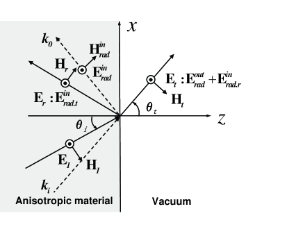
Figure 6: Schematic diagram for how the reflected and transmitted fields are generated for TE waves incident from an anisotropic material into vacuum. The process is distinct from those in external reflection as in Fig. 1. Under the action of the incident field ${\bf E}_{1}$, the dipoles produce an internal radiated field ${\bf E}_{rad}^{in}$ in the material and an external one ${\bf E}_{rad}^{out}$ in the vacuum. ${\bf E}_{rad}^{in}$ can be regarded as an incident wave from the vacuum into the material. It produces a reflected wave ${\bf E}_{rad.r}^{in}$ in the vacuum and a transmitted wave ${\bf E}_{rad.t}^{in}$ in the material. The magnitude of the real reflected field is ${\bf E}_{r0}={\bf E}_{rad.t}^{in}=T{\bf E}_{rad}^{in}$. The final transmitted field is ${\bf E}_{t0}={\bf E}_{rad.r}^{in}+{\bf E}_{rad}^{out}$. When ${\bf E}_{rad}^{in}={\bf E}^{e}_{rad}+{\bf E}^{m}_{rad}=0$, ${\bf E}_{r0}=0$ and Brewster angle occurs.

III.2 Brewster angle

Next, we explore the mechanism of Brewster angle in internal reflection.

In order to satisfy $r_{E}=|{\bf E}_{r0}/{\bf E}_{10}|^{2}=0$, it requires ${\bf E}^{in}_{rad}=0$ in Eq. (29). Equation (27) is similar to Eq. (12), then one can obtain conclusions similar to those about Brewster angle for external reflection in the subsection B of Sec. II after replacing $k_{iz}$ and $k_{tz}$ with $k_{tz}$ and $k_{1z}$, respectively. Thus the conditions for Brewster angle in internal reflection are identical to those of external reflection. The Brewster angle of internal reflection can be obtained by Snell’s law $\sin{\theta_{B}}=k_{t}\sin{\theta_{t}}/{k_{1}}$, where $\theta_{t}$ is equal to the Brewster angle of external reflection. Therefore, we know that if the condition

$$0<\frac{1-\frac{\mu_{0}\varepsilon_{y}}{\mu_{x}\varepsilon_{0}}}{1-\frac{\mu_{0}\mu_{0}}{\mu_{x}\mu_{z}}}<1$$ (34)

is satisfied, the Brewster angle for TE waves is

$$\theta_{B}^{TE}=\sin^{-1}\sqrt{\frac{\mu_{0}\mu_{z}(\varepsilon_{y}\mu_{0}-\varepsilon_{0}\mu_{x})}{\varepsilon_{0}\mu_{0}(\mu_{x}^{2}-\mu_{x}\mu_{z})+\varepsilon_{y}\mu_{z}(\mu_{0}^{2}-\mu_{x}^{2})}}.$$ (35)

Similarly, we conclude that under the condition

$$0<\frac{1-\frac{\varepsilon_{0}\mu_{y}}{\varepsilon_{x}\mu_{0}}}{1-\frac{\varepsilon_{0}\varepsilon_{0}}{\varepsilon_{x}\varepsilon_{z}}}<1,$$ (36)

there exists a Brewster angle for TM waves

$$\theta_{B}^{TM}=\sin^{-1}\sqrt{\frac{\varepsilon_{0}\varepsilon_{z}(\mu_{y}\varepsilon_{0}-\mu_{0}\varepsilon_{x})}{\varepsilon_{0}\mu_{0}(\varepsilon_{x}^{2}-\varepsilon_{x}\varepsilon_{z})+\mu_{y}\varepsilon_{z}(\varepsilon_{0}^{2}-\varepsilon_{x}^{2})}}.$$ (37)

Through choosing appropriate material parameters, i.e., ${\bm{\varepsilon}}$ and ${\bm{\mu}}$, Brewster angles can happen to both TE and TM waves. Since the requirements on ${\bm{\varepsilon}}$ and ${\bm{\mu}}$ for Brewster angle in internal reflection are the same as those in external reflection, we can discuss and come to conclusions about the Brewster angle in internal reflection similar to in external reflection.

IV Conclusion

In summary, we have used the extinction theorem to generalize the existence condition of Brewster angle from the isotropic dielectric material to the anisotropic dielectric-magnetic material. We investigated the Brewster angle not only in external reflection, but also in internal reflection. We found the mechanism for Brewster effect is that the total contributions of the anisotropic material’s electric and magnetic dipoles to the reflection fields are zero. Interestingly, the requirements on the material parameters ${\bm{\varepsilon}}$ and ${\bm{\mu}}$ for Brewster angle in internal reflection are the same as those in external reflection, and the corresponding Brewster angle is just the refracted angle of external reflection at the incidence of external Brewster angle. This point is consistent with the reversibility of light ray. We also discussed in detail the impact of ${\bm{\varepsilon}}$ and ${\bm{\mu}}$ on the Brewster angle. We found that, through choosing appropriate ${\bm{\varepsilon}}$ and ${\bm{\mu}}$ the anisotropic material can exhibit Brewster angles for TE waves, or TM waves, or both. Moreover, the Brewster effect can happen to TE and TM waves simultaneously and the omnidirectional total transmission will occur, which may lead to important applications in practice.

Although based on molecular optics theory, these conclusions are applicable to metamaterials consisting of SRRs and wires. That is because both the SRR and the wire dimensions are much smaller than the wavelength of interest Shelby2001 . Then the unit cells of SRR and wire can be modelled as the molecules (or atoms) in ordinary materials. Actually, Belov et al. have used the Ewald-Oseen extinction theorem to investigate the boundary problem of metamaterials Belov2006 . We hope that our results will provide references in manufacturing materials for specific purposes, such as making polarization devices.

References

• (1) M. Born and E. Wolf, Principles of Optics, 7th ed. (Cambridge, Cambridge, 1999).
• (2) V. G. Veselago, Sov. Phys. Usp. 10, 509 (1968).
• (3) R. A. Shelby, D. R. Smith, and S. Schultz, Science 292, 77 (2001).
• (4) J. B. Pendry, Phys.Β Rev.Β Lett.Β 85, 3966 (2000).
• (5) I. V. Lindell, S. A. Tretyakov, K. I. Nikoskinen, and S. Ilvonen, Microw. Opt. Technol. Lett. 31, 129 (2001).
• (6) D. R. Smith and D. Schurig, Phys.Β Rev.Β Lett.Β 90, 077405 (2003).
• (7) D. R. Smith, P. Kolinko, and D. Schurig, J. Opt. Soc. Am. B 21, 1032 (2004).
• (8) C. Luo, S. G. Johnson, J. D. Joannopoulos, and J. B. Pendry, Optics Express 11, 746 (2003).
• (9) L. B. Hu, S. T. Chui, Phys.Β Rev.Β B66, 085108 (2002).
• (10) P. A. Belov, Microw. Opt. Technol. Lett. 37, 259–263 (2003).
• (11) Tom G. Mackay and A. Lakhtakia, Phys.Β Rev.Β E69, 026602 (2004)
• (12) R. A. Depine, M. E. Inchaussandague, A. Lakhtakia, J. Opt. Soc. Am. A. 23, 949 (2006).
• (13) H. Luo, W. Hu, X. Yi, H. Liu, and J. Zhu, Opt.Β Commun.Β  254, 353 (2005).
• (14) H. Luo, W. Hu, W. Shu, F. Li and Z. Ren, Europhys. Lett. 74, 1081 (2006).
• (15) L. Zhou, C. T. Chan, and P. Sheng, Phys.Β Rev.Β B68, 115424 (2003).
• (16) T. M. Grzegorczyk, Z. M. Thomas, and J. A. Kong, Appl.Β Phys.Β Lett.Β 86, 251909 (2005).
• (17) R. P. Feynman, R. B. Leighton, and M. Sands, The Feynman Lectures on Physics (Addison-Wesley, 1963), Vol. 1, Secs. 31 and 30-7.
• (18) E. Lalor and E. Wolf, J. Opt. Soc. Am. 62, 1165 (1972).
• (19) M. A. Karam, Applied Optics. 36, 5238–5245 (1997).
• (20) G. C. Reali, J. Opt. Soc. Am. 72, 1421 (1982).
• (21) W. T. Doyle, Am. J. Phys. 53, 463 (1985).
• (22) H. M. Lai, Y. P. Lau, and W. H. Wong, Am. J. Phys. 70, 173 C179 (2002).
• (23) C. Fu, Z. M. Zhang, and P. N. First, Applied Optics. 44, 3716 (2005).
• (24) M. A. Karam, J. Opt. Soc. Am. A 13, 2208 (1996).
• (25) N. H. Shen, Q. Wang, J. Chen, Y. X. Fan, J. P. Ding, H. T. Wang, J. Opt. Soc. Am. B. 23, 904 (2006).
• (26) J. A. Kong, Electromagnetic wave theory (EMW, New York, 2000).
• (27) P. A. Belov, Phys.Β Rev.Β B73, 045102 (2006).