Queueing theoretical analysis of foreign currency exchange rates

Abstract

We propose a useful approach for investigating the statistical properties of foreign currency exchange rates. Our approach is based on queueing theory, particularly, the so-called renewal-reward theorem. For the first passage processes of the Sony Bank US dollar/Japanese yen (USD/JPY) exchange rate, we evaluate the average waiting time which is defined as the average time that customers have to wait between any instant when they want to observe the rate (e.g. when they log in to their computer systems) and the next rate change. We find that the assumption of exponential distribution for the first-passage process should be rejected and that a Weibull distribution seems more suitable for explaining the stochastic process of the Sony Bank rate. Our approach also enables us to evaluate the expected reward for customers, i.e. one can predict how long customers must wait and how much reward they will obtain by the next price change after they log in to their computer systems. We check the validity of our prediction by comparing it with empirical data analysis.

I Introduction

Recently, internet trading has become very popular. Obviously, the rate (or price) change of the trading behaves according to some unknown stochastic processes, and numerous studies have been conducted to reveal the statistical properties of its nonlinear dynamics Mantegna2000 ; Bouchaud ; Voit . In fact, several authors have analysed tick-by-tick data of price changes including the currency exchange rate in financial markets Simonsen ; Simonsen2 ; Raberto ; Scalas ; Kurihara ; Sazuka ; Sazuka2 . Some of these studies are restricted to the stochastic variables of price changes (returns) and most of them are specified by terms such as the fat or heavy tails of distributions Mantegna2000 . However, fluctuation in time intervals, namely, the duration in the point process Cox1 ; Cox2 might also contain important market information, and it is worthwhile to investigate these properties.

Such fluctuations in the time intervals between events are not unique to price changes in financial markets but are also very common in the real world. In fact, it is wellknown that the spike train of a single neuron in the human brain is regarded as a time series, wherein the difference between two successive spikes is not constant but fluctuates. The stochastic process specified by the so-called inter-spike intervals (ISI) is one such example Tuckwell ; Gerstner . The average ISI is of the order of a few milli-second and the distribution of the intervals is well-described by a Gamma distribution Gerstner .

On the other hand, in financial markets, for instance, the time interval between two consecutive transactions of Bund futures (Bund is the German word for bond) and BTP futures (BTPs are middle- and long-term Italian Government bonds with fixed interest rates) traded at London International Financial Futures and Options Exchange (LIFFE) is $\sim 10$ seconds and is well-fitted by the Mittag-Leffler function Mainardi ; Raberto ; Scalas . The Mittag-Leffler function behaves as a stretched exponential distribution for short time-interval regimes, whereas for the long time-interval regimes, the function has a power-law tail. Thus, the behaviour of the distribution described by the Mittag-Leffler function changes from the stretched exponential to the power-law at some critical point Gorenflo . However, it is nontrivial to determine whether the Mittag-Leffler function supports any other kind of market data, e.g. the market data filtered by a rate window.

Similar to the stochastic processes of price change in financial markets, the US dollar/Japanese yen (USD/JPY) exchange rate of Sony Bank Sony , which is an internet-based bank, reproduces its rate by using a rate window with a width of $0.1$ yen for its individual customers in Japan. That is, if the USD/JPY market rate changes by more than $0.1$ yen, the USD/JPY Sony Bank rate is updated to the market rate. In this sense, it is possible for us to say that the procedure of determination of the Sony Bank USD/JPY exchange rate is essentially a first-passage process Redner ; Kappen ; Risken ; Gardiner ; Schoutens .

In this paper, we analyse the average time interval that a customer must wait until the next price (rate) change after they log in to their computer systems. Empirical data analysis has shown that the average time interval between rate changes is one of the most important statistics for understanding market behaviour. However, as internet trading becomes popular, customers would be more interested in the average waiting time — defined as the average time that customers have to wait between any instant and the next price change — when they want to observe the rate, e.g. when they log in to their computer systems rather than the average time interval between rate changes. To evaluate the average waiting time, we use the so-called renewal-reward theorem which is wellknown in the field of queueing theory Tijms ; Oishi . In addition, we provide a simple formula to evaluate the expected reward for customers. In particular, we investigate these important quantities for the Sony Bank USD/JPY exchange rate by analysing a simple probabilistic model and computer simulations that are based on the ARCH (autoregressive conditional heteroscedasticity) Engle and GARCH (generalised ARCH) Mantegna2000 ; Ballerslev ; Franke stochastic models with the assistance of empirical data analysis of the Sony Bank rate Sazuka ; Sazuka2 .

This paper is organised as follows. In the next section, we explain the method being used by the Sony Bank and introduce several studies concerning empirical data about the rate. In Sec. III, we introduce a general formula to evaluate average waiting time using the renewal-reward theorem and calculate it with regard to Sony Bank customers. Recently, one of the authors Sazuka2 provided evidence implying that the first-passage time (FPT) distribution of the Sony Bank rate obeys the Weibull distribution Everitt . This conjecture is regarded as a counter part of studies that suggest that the FPT should follow an exponential distribution (see example in Chan ). In the same section, we evaluate the average waiting time while assuming that FPT obeys an exponential distribution. Next, we compare it with the result for the Weibull distribution and perform empirical data analyses Sazuka ; Sazuka2 . We find that the assumption of exponential distributions on the first-passage process should be rejected and that a Weibull distribution seems more suitable for explaining the first-passage processes of the Sony Bank rate. Thus, we can predict how long customers wait and how many returns they obtain until the next rate change after they log in to their computer systems. In Sec. IV, to investigate the effects of the rate window of the Sony Bank, we introduce the ARCH and GARCH models to reproduce the raw data before filtering it through the rate window. In Sec. V, we evaluate the reward that customers can expect to obtain after they log in to their computer systems. The last section provides a summary and discussion.

II Data: The Sony Bank USD/JPY exchange rate

The Sony Bank rate Sony is the foreign exchange rate that the Sony Bank offers with reference to the market rate and not their customers’ orders. In FIG. 1, we show a typical update of the Sony Bank rate.

Figure 1: The Sony Bank USD/JPY exchange rate. The units of the horizontal and vertical axes are ticks and yen/dollar, respectively.

If the USD/JPY market rate changes by greater than or equal to $0.1$ yen, the Sony Bank USD/JPY rate is updated to the market rate. In FIG. 2, we show the method of generating the Sony Bank rate from the market rate.

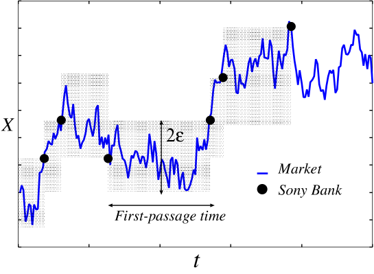
Figure 2: An illustration of generating the filtered rate (black circle) by the rate window with a constant width $2\epsilon$ in time (shaded area) from the market rate (solid line). The units of the horizontal and the vertical axes are ticks and yen, respectively.

In this sense, the Sony Bank rate can be regarded as a kind of first-passage processes. In TABLE 1, we show data concerning the Sony Bank USD/JPY rate vs. tick-by-tick data for the USD/JPY rate from Bloomberg L.P.

Table 1: The Sony Bank USD/JPY rate vs. tick-by-tick data for the USD/JPY rate Sazuka .

	Sony Bank rate	tick-by-tick data
Number of data per day	$\sim 70$	$\sim 10,000$
The smallest price change	$0.1$ yen	$0.01$ yen
Average interval between data	$\sim 20$ minutes	$\sim 7$ seconds

From these tables and figures, an important question might arise. Namely; how long should Sony Bank customers wait between observing the price and the next price change? This type of question never arises in the case of ISI or Bund futures, because the average time intervals are too short to evaluate such measures. We would like to stress that in this paper, we do not discuss the market data underlying the Sony Bank rate; however, as we will see in the following sections, the main result obtained in this study, i.e. how long a trader must wait for the next price change of the Sony Bank rate from the time she or he logs on to the internet, is not affected by this lack of information.

III Renewal-reward theorem and average waiting time

From TABLE 1, we find that the number of data per day is remarkably reduced from $\sim 10,000$ to $\sim 70$ because of an effect of the rate window of $0.1$-yen width. As a result, the average interval of exchange rate updates is extended to $\sim 20$ min. This quantity is one of the most important measures for the market, however, customers might seek information about the average waiting time, which is defined as the average time interval that customers have to wait until the next change of the Sony Bank USD/JPY rate after they log in to their computer systems. To evaluate the average waiting time, we use the renewal-reward theorem, which is wellknown in the field of queueing theory Tijms ; Oishi . We briefly explain the theorem below.

Let us define $N(\tau)$ as the number of rate changes within the interval $(0,\tau]$ and suppose that a customer logs in to her/his computer system at time $\tau$ ($\tau_{N(\tau)}\leq\tau<\tau_{N(\tau)+1}$). Then, we defined the following quantity:

$$W(\tau) = \tau_{N(\tau)+1}-\tau,$$ (1)

which denotes the waiting time for the customer until the next update of the Sony Bank USD/JPY rates when she or he logs in to a computer system at time $\tau$. Then, the renewal-reward theorem Tijms ; Oishi implies that the average waiting time $w$ can be written in terms of the first two moments, $E(t)$ and $E(t^{2})$, of the first-passage time distribution $P(t)$ as

$$w = \lim_{\tau\to\infty}\frac{1}{\tau}\int_{0}^{\tau}W(s)ds=\frac{E(t^{2})}{2E(t)},$$ (2)

where $E(\cdots)$ denotes $\int_{0}^{\infty}dt(\cdots)P(t)$. Therefore, if we obtain the explicit form of the FPT distribution $P(t)$, we can evaluate the average waiting time $w$ by using this theorem (2).

The proof of the theorem is quite simple. Let us suppose that the points at which the Sony Bank USD/JPY rate changes are given by the time sequence $\tau_{1},\tau_{2},\cdots,\tau_{N(\tau)}$. For these data points, the first-passage time series is given by definition as $t_{0}=\tau_{1},t_{1}=\tau_{2}-\tau_{1},t_{2}=\tau_{3}-\tau_{2},\cdots,t_{N(\tau)-1}=\tau_{N(\tau)}-\tau_{N(\tau)-1}$. Then, we observe that the time integral $\int_{0}^{\tau}W(s)ds$ appearing in equation (2) is identical to $\sum_{i=0}^{N(\tau)}(t_{i})^{2}/2$, where $(t_{i})^{2}/2$ corresponds to the area of a triangle with sides $t_{i},t_{i}$ and $\sqrt{2}\,t_{i}$. As a result, we obtain

$$w = \lim_{\tau\to\infty}\frac{1}{\tau}\int_{0}^{\tau}W(s)ds\,\simeq\,\frac{N(\tau)}{\tau}\cdot\frac{1}{N(\tau)}\sum_{i=1}^{N(\tau)}\frac{(t_{i})^{2}}{2}=\frac{E(t^{2})}{2E(t)},$$ (3)

wherein we used the fact that the expectation of the waiting time $t_{i}$ is given by

$$E(t) = \frac{1}{N(\tau)}\sum_{i=0}^{N(\tau)}t_{i}=\frac{1}{N(\tau)}\{\tau_{1}+\tau_{2}-\tau_{1}+\tau_{3}-\tau_{2}+\cdots+\tau_{N(\tau)}-\tau_{N(\tau)-1}\}=\frac{\tau_{N(\tau)}}{N(\tau)}.$$ (4)

Therefore,

$$\lim_{\tau\to\infty}\frac{N(\tau)}{\tau} = \frac{1}{E(t)}.$$ (5)

Thus, equation (2) holds true.

Therefore, if we obtain the explicit form of the first-passage time distribution $P(t)$, the average waiting time $w$ can be evaluated by theorem (2). However, for estimating the distribution $P(t)$, we can only perform empirical data analysis of the Sony Bank rate. Apparently, the first-passage process of the Sony Bank rate depends on the stochastic processes of raw market data underlying the data that is available on the website for customers after being filtered by a rate window of $0.1$-yen width. Unfortunately, this raw data is not available to us and we cannot use any information regarding the high-frequency raw data.

Recently, an empirical data analysis by one of the authors of this paper Sazuka2 revealed that the Weibull probability distribution function, which is defined by

$$P_{W}(t) = m\,\frac{t^{m-1}}{a}\,{\exp}\left(-\frac{t^{m}}{a}\right),$$ (6)

is a good approximation of the Sony Bank USD/JPY rate in the non-asymptotic regime. We should keep in mind that in the asymptotic regime, the FPT distribution obeys the power-law — $P(t)\,\sim\,t^{-\alpha}\,\,(\alpha\sim 3.67)$ — and a crossover takes place at the intermediate time scale $t_{\rm c}\,\sim\,18,000$ [s]. However, the percentage of empirical data for the power-law regime is only $0.3\%$. Similar behaviour was observed for the time-interval distribution between two consecutive transactions of Bund futures traded at LIFFE, and the time-interval distribution is well-described by the Mittag-Leffler type function Mainardi , namely, the distribution changes from the stretched exponential to the power-law for long-time regimes. Therefore, we have chosen a Weibull distribution in both asymptotic and non-asymptotic regimes to evaluate the average waiting time. The justification for this choice will be discussed later by comparing the predicted value with the result from empirical data analysis.

This Weibull distribution (6) is reduced to an exponential distribution for $m=1$ and a Rayleigh distribution for $m=2$. It is easy for us to evaluate the first two moments of the distribution $P_{W}(t)$. We obtained them explicitly as $E(t)=a^{1/m}\Gamma(1+(1/m))$ and $E(t^{2})=a^{2/m}\Gamma(1+(2/m))$. Thus, the average waiting time $w$ for the Weibull distribution is explicitly given by

$$w = a^{1/m}\,\frac{\Gamma\left(\frac{2}{m}\right)}{\Gamma\left(\frac{1}{m}\right)},$$ (7)

where $\Gamma(z)$ refers to the gamma function, and $\Gamma(z+1)=z\Gamma(z)$.

Figure 3: Average waiting time $w$ as a function of $m$ for the Weibull distribution. We set $a=0.5,1$ and $2$. The unit of the vertical axis is second. In the inset, we plot for $a=50.855$, which was evaluated from empirical data of the Sony Bank USD/JPY rate Sazuka2 . From the inset, for the parameter $m=0.59$, the average waiting time $w$ is expected to be $w\simeq 2534.146\,\,\mbox{[s]}=42.236$ [min]. This time interval does not differ much from the result ($w\sim 49$ [min]) obtained from our empirical data analysis.

In FIG. 3 we plot the average waiting time $w$ (7) as a function of $m$ for several values of $a$, and we find that $w$ for Sony Bank customers is convenient and reasonable. This is because the empirical data analysis reported the value of the parameter as $m=0.59$, and the average waiting time $w$ for this case is evaluated as $w\simeq 2534.146\,\,\mbox{[s]}=42.236$ [min] from the inset of this figure. From reference Sazuka2 , information about the scaling parameter $a$ was not available; however, we can easily obtain the value as discussed next.

As mentioned above, several empirical data analyses Sazuka2 revealed that parameter $m\simeq 0.59$ for the Sony Bank rate. In fact, it is possible for us to estimate $a$ by using the fact that the average interval $\langle t\rangle$ of the rate change is $\sim 20$ [min] (TABLE 1). Next, we obtain the following simple relation:

$$E(t) = \langle t\rangle.$$ (8)

That is $(a^{1/m}/{m})\Gamma(1/m)=\langle t\rangle$. Therefore,

$$a = \left\{\frac{m\langle t\rangle}{\Gamma\left(\frac{1}{m}\right)}\right\}^{m}.$$ (9)

Substituting $m\simeq 0.59$ and $\langle t\rangle\sim 20\times 60=1200$ [s], we obtain the parameter $a$ for the Sony Bank rate as $a\simeq 50.855$.

It should be noted that the average waiting time is also evaluated by a simple sampling from the empirical data of the Sony Bank rates. The first two moments of the first-passage time distribution $P_{W}(t)$ — $\langle t\rangle\equiv\lim_{T\to\infty}(1/T)\sum_{k=0}^{T}\Delta t_{k},\langle t^{2}\rangle\equiv\lim_{T\to\infty}(1/T)\sum_{k=0}^{T}(\Delta t_{k})^{2}$ — are easily calculated from the sampling, and then, the average waiting time is given by $w_{\rm sampling}=\langle t^{2}\rangle/2\langle t\rangle$. We find that $w_{\rm sampling}\simeq 49$ [min] which is not much different from that obtained by evaluation ($w=42.236$ [min]) by means of the renewal-reward theorem (2). Thus, the renewal-reward theorem introduced here determines the average waiting time of the financial system with adequate accuracy, and our assumption of the Weibull distribution for the first-passage time of the Sony Bank rates seems to be reasonable. We would particularly like to stress that the $0.3\%$ data from the asymptotic regime does not contribute much to the average waiting time.

A detailed account of this fine agreement between $w$ and $w_{\rm sampling}$, more precisely, the factors to which we can attribute the small difference between $w$ and $w_{\rm sampling}$, will be reported in our forthcoming paper ISE .

We would now like to discuss the average waiting time for the case in which the first-passage process can be regarded as a Poisson process. In the Poisson process, the number of events occurring in the interval $(0,\tau]$ is given by $P_{k}(\tau)=(\lambda\tau)^{k}\,{\rm e}^{-\lambda\tau}/k!$   $(k=0,1,2,\cdots)$. For this Poisson process, the time interval $t$ between two arbitrary successive events obeys the following exponential distribution:

$$P(t) = \lambda\,{\rm e}^{-\lambda t}.$$ (10)

Then, we obtain the first two moments of the above distribution $P(t)$ as $E(t)=1/\lambda,E(t^{2})=2/\lambda^{2}$. These two moments give the average waiting time for the Poisson process as $w=E(t^{2})/2E(t)=1/\lambda=E(t)$. Therefore, for the Poisson process, the average waiting time $w$ is identical to the average rate interval $E(t)$. This result might be naturally accepted because the login-time dependence on the average waiting time is averaged out due to the fact that for a Poisson process, each event takes place independently. On the other hand, for a non-Poisson process, the login time is essential to determine the average waiting time. Thus, the average waiting time becomes $E(t^{2})/2E(t)$ instead of $E(t)$.

We should stress that for a given stochastic process whose FPT is a constant $T$, the average waiting time $w$ is easily evaluated by $w=(1/T)\int_{0}^{T}sds=T/2$. However, the result for the above Poisson process implies that for a Poisson process with a mean $E(t)$ of the FPT, the average waiting time is not $E(t)/2$ but $E(t)$. This fact is referred to as the inspection paradox Tijms in the field of queueing theory. For a Poisson process, each event occurs independently, but the time interval between the events follows an exponential distribution. Therefore, there is some opportunity for the customers to log in to their computer systems when the exchange rate remains the same for a relatively long time, although the short FPT occurs with higher frequency than the long FPT. This fact makes $w$ the first moment $E(t)$ of the FPT distribution.

On the other hand, for the Weibull distribution, the condition under which the average waiting time $w$ is the same as the average first-passage time $E(t)$ is given by $w=E(t)$, i.e.

$$m\Gamma\left(\frac{2}{m}\right) = \left\{\Gamma\left(\frac{1}{m}\right)\right\}^{2}.$$ (11)

Figure 4: $m\Gamma(2/m)$ and $\{\Gamma(1/m)\}^{2}$ as functions of $m$. The crossing point $m_{\times}=1$ of the two curves corresponds to the Weibull parameter for which the average waiting time $w$ is identical to the average first-passage time $E(t)$. For $m<m_{\times}$ (the case of Sony Bank), $w>E(t)$ holds true, whereas for $m>m_{\times}$, $w<E(t)$ is satisfied.

In FIG. 4, we plot both curves $m\Gamma(2/m)$ and $\{\Gamma(1/m)\}^{2}$, as functions of $m$. The crossing point $m_{\times}=1$ corresponds to the Weibull parameter for which the average waiting time $w$ is identical to the average first-passage time $E(t)$. Obviously, for the parameter regime $m<m_{\times}$ (the case of Sony Bank), the average waiting time evaluated by the renewal-reward theorem becomes longer than the average first-passage time $E(t)$. As mentioned before, the Weibull distribution with $m=1$ follows the exponential distribution $P_{W}(t)\,\sim\,{\rm e}^{-t}$. Therefore, as mentioned in the case of the Poisson process, the login-time dependence of the customers is averaged out in the calculation of the average waiting time $w$. As the result, $w$ becomes the first moment of the FPT distribution, $E(t)$. However, once the parameter of the Weibull distribution has deviated from $m=m_{\times}=1$, the cumulative distribution is no longer an exponential distribution. Thus, the stochastic process is not described by a Poisson process and the average waiting time $w$ is not $E(t)$ but $w=E(t^{2})/2E(t)$ which is derived from the renewal-reward theorem. As mentioned above, the empirical data analysis revealed that the average waiting time of Sony Bank rates is $w_{sampling}=\langle t^{2}\rangle/2\langle t\rangle\sim 49$ [min]. This value is almost twice of the average interval of the rate change data $E(t)=\langle t\rangle\,\sim\,20$ [min] in TABLE 1. This fact is a kind of justification or evidence for the conclusion that the Sony Bank USD/JPY exchange rate obeys non-exponential distribution from the viewpoint of the renewal-reward theorem.

IV Effect of rate window on first-passage processes of price change

In the previous sections, we evaluated the average waiting time $w$ for foreign exchange rates (price change). In particular, we focused on the average waiting time of the Sony Bank rate whose FPT distribution might be represented by a Weibull distribution. We compared the average waiting time $w$ obtained by the renewal-reward theorem with that obtained by a simple sampling of the empirical data of the Sony Bank rate and found a good agreement between the two. However, as mentioned earlier, the empirical data of Sony Bank was obtained by filtering the raw market data using a rate window of $0.1$-yen width. Unfortunately, the raw data of the real market is not available to us (Sony Bank does not keep these records) and the only information we could obtain is the Sony Bank rate itself. Although the main result of the evaluation of the average waiting time is never affected by this lack of information, it might be worthwhile to investigate the role of the rate window with the assistance of computer simulations.

For this purpose, we introduce the stochastic process $X_{k_{0}},X_{k_{1}},\cdots,X_{k_{n}},\cdots$ , where the time intervals of two successive time stamps $\Delta t_{1}=k_{1}-k_{0},\Delta t_{2}=k_{2}-k_{1},\cdots,\Delta t_{n}=k_{n}-k_{n-1},\cdots$ obey a Weibull distribution specified by the two parameters $m_{0}$ and $a_{0}$. For example, for the ordinary Wiener process, the above stochastic process is described by

$$X_{t+\Delta t} = X_{t}+Y_{t},\,\,\,\,\,Y_{t}={\cal N}(0,\sigma^{2}),$$ (12)

$$P_{W}^{0}(\Delta t) = m_{0}\,\frac{(\Delta t)^{m_{0}-1}}{a_{0}}{\exp}\left(-\frac{(\Delta t)^{m_{0}}}{a_{0}}\right),$$ (13)

where $X_{t}$ denotes the value of price at time $t$. Obviously, the first-passage time of the above stochastic process has a distribution $P(t)$, which is generally different from $P_{W}^{0}(\Delta t)$. Nevertheless, here we assume that $P(t)$ also obeys a Weibull distribution with parameters $m$ and $a$. Next, we investigate the effect of a rate window with a width of $\epsilon$ through the difference of the parameters, namely, the $m$-$m_{0}$ and $a$-$a_{0}$ plots. For simplicity, we set $a=a_{0}=1$ in our computer simulations. In other words, using computer simulations, we clarify the relationship between the input $m_{0}$ and the corresponding output $m$ of the filter with a rate window of width $\epsilon$.

IV.1 The Weibull paper analysis of the FPT distribution

To determine the output $m$ from the histogram of first-passage time, we use the Weibull paper analysis Sazuka2 ; Everitt for cumulative distribution. Now, we briefly explain the details of the method.

We first consider the cumulative distribution of the Weibull distributions with $a=1$ as

$$R(t) = \int_{t}^{\infty}P_{W}(s)ds=\exp(-t^{m}).$$ (14)

Then, for the histogram of the cumulative distribution obtained by sampling using computer simulations, we fit the histogram to the Weibull distribution by using the following Weibull paper:

$$\log\{\log(R(t)^{-1})\} = m\log t.$$ (15)

Thus, the parameter $m$ of the first-passage time distribution $P(t)$ is obtained as a slope of the $\log t$-$\log\log(R(t)^{-1})$ plot. In the following subsection, we evaluate the parameter $m$ of the FPT distribution for the stochastic processes with time intervals of two successive time stamps $\Delta t$ obeying the Weibull distribution $P_{W}^{0}(\Delta t)$. Then, we compare $m_{0}$ with $m$ using the above Weibull paper analysis (15).

IV.2 ARCH and GARCH processes as stochastic models for raw market data

As stochastic model of the raw data of the real market, the Wiener process defined by equations (12) and (13) is one of the simplest candidates. However, numerous studies from both empirical and theoretical viewpoints have revealed that the volatility of financial data such as the USD/JPY exchange rate is a time-dependent stochastic variable. With this fact in mind, we introduce two types of stochastic processes that are characterised by time-dependent volatility — ARCH Engle and GARCH models Mantegna2000 ; Engle ; Franke .

The ARCH(1) model used in this section is described as follows:

$$\sigma_{t+\Delta t}^{2} = \alpha_{0}+\alpha_{1}X_{t}^{2},$$ (16)

$$X_{t+\Delta t} = X_{t}+{\cal N}(0,\sigma_{t}^{2}),$$ (17)

where we assume that the time interval $\Delta t$ obeys the Weibull distribution (13). From the definition in (16) and (17), we find that the volatility $\sigma_{t}^{2}$ controlling the conditional probability density $P(X_{t})$ at time $t$ fluctuates. However, for the limit $t\to\infty$, such a local time dependence does not prevent the stochastic process from having a well-defined asymptotic distribution $P(X)$. In fact, the above ARCH(1) model is characterised by the variance $\sigma^{2}$ observed over a long time interval $t\to\infty$. It is easily shown that $\sigma^{2}$ can be written in terms of $\alpha_{0}$ and $\alpha_{1}$ as

$$\sigma^{2} = \frac{\alpha_{0}}{1-\alpha_{1}}.$$ (18)

We choose the parameters $\alpha_{0}$ and $\alpha_{1}$ so as to satisfy $\sigma=\epsilon=1$. As a possible choice for this requirement, we select $(\alpha_{0},\alpha_{1})=(0.45,0.55)$. For this parameter choice, the kurtosis (${\rm Kurt}$), which is defined by the second and fourth moments of the probability distribution function of the stochastic variable $X$ as $\langle X^{4}\rangle/\langle X^{2}\rangle^{2}$, leads to

$${\rm Kurt} = 3+\frac{6\alpha_{1}^{2}}{1-3\alpha_{1}^{2}}.$$ (19)

As is well-known, the higher kurtosis values of financial data indicate that the values close to the mean and extreme positive and negative outliers appear more frequently than for normally distributed variables. In other words, the kurtosis is a measure of the fatness of the tails of the distribution. For instance, a normal Gaussian distribution has ${\rm Kurt}=0$, whereas distributions with ${\rm Kurt}>0$ are referred to as leptokurtic and have tails fatter than a Gaussian distribution. The kurtosis of the ARCH(1) model with $(\alpha_{0},\alpha_{1})=(0.45,0.55)$ is ${\rm Kurt}=23$.

Here, we also introduce the GARCH(1,1) model defined as

$$\sigma_{t+\Delta t}^{2} = \alpha_{0}+\alpha_{1}X_{t}^{2}+\beta_{1}\sigma_{t}^{2},$$ (20)

$$X_{t+\Delta t} = X_{t}+{\cal N}(0,\sigma_{t}^{2}),$$ (21)

where the time interval $\Delta t$ is assumed to obey the Weibull distribution (13). The variance of the above GARCH(1,1) model observed on a long time interval, $t\to\infty$, is given by

$$\sigma^{2} = \frac{\alpha_{0}}{1-\alpha_{1}-\beta_{1}}.$$ (22)

To compare the effect of the rate window for the ARCH(1) model with that of the GARCH(1,1) model, we choose the parameters $\alpha_{0},\alpha_{1}$ and $\beta_{1}$ so as to satisfy $\sigma=\epsilon=1$. Among many candidates, we select $(\alpha_{0},\alpha_{1},\beta_{1})=(0.4,0.3,0.3)$, which gives the kurtosis

$${\rm Kurt} = 3+\frac{6\alpha_{1}^{2}}{1-3\alpha_{1}^{2}-2\alpha_{1}\beta_{1}-\beta_{1}^{2}}=4.17.$$ (23)

Figure 5: Probability density function of successive increments (return) $Y=X_{t+\Delta t}-X_{t}$. The unit of the horizontal axis is yen. The left panel is the PDF for the ARCH(1) model with $(\alpha_{0},\alpha_{1})=(0.45,0.55)$ and ${\rm Kurt}=23$. The right panel is the PDF for the GARCH(1,1) model with $(\alpha_{0},\alpha_{1},\beta_{1})=(0.4,0.3,0.3)$ and ${\rm Kurt}=4.17$. In both panels, the broken line corresponds to the PDF for a normal Gaussian ${\cal N}(0,1)$.

In FIG. 5, We plot the probability density function (PDF) of the successive increments (returns) $Y=X_{t+\Delta t}-X_{t}$ for the ARCH(1) and the GARCH(1,1) models. The left panel is the PDF for the ARCH(1) with $(\alpha_{0},\alpha_{1})=(0.45,0.55)$ and ${\rm Kurt}=23$. The right panel is the PDF for the GARCH(1,1) model with $(\alpha_{0},\alpha_{1},\beta_{1})=(0.4,0.3,0.3)$ and ${\rm Kurt}=4.17$.

For the stochastic processes for modelling the raw real market data, namely, the Winer process and the ARCH(1) and GARCH(1,1) models, we determine the parameter $m$ for each FPT distribution by means of the Weibull paper analysis based on (15), and then plot the $m_{0}$-$m$ relation for each stochastic model.

Figure 6: The $m_{0}$-$m$ relations for the Wiener process and the ARCH(1) and GARCH(1,1) models (left). The right panel shows the $m_{0}$-dependence of the average waiting time $w$ for each stochastic process. In this panel, the unit of the vertical axis is second. Each error-bar is evaluated by $20$ independent runs.

In the left panel of FIG. 6, we plot the $m_{0}$-$m$ relations for the stochastic processes: the Wiener process and the ARCH(1) and GARCH(1,1) models. In this panel, the crossing point between the line $m=m_{0}$ and each plot indicates the value of $m_{0}$ for which the distribution $P(t)$ of the first-passage time remains the same as that of the time interval $\Delta t$ of the raw data $P_{W}^{0}(\Delta t)$. Therefore, below the line $m=m_{0}$, the rate window affects the stochastic process so as to decrease the parameter $m_{0}$ of the Weibull distribution, whereas, above this line, the parameter $m_{0}$ increases to $m\,(>m_{0})$. As mentioned earlier, empirical data analysis of the Sony Bank rate Sazuka2 suggested that the waiting time or the time interval $\Delta t$ of the Sony Bank rate obeys the Weibull distribution with $m=0.59$. Therefore, there is a possibility that the raw data before applying the rate window could be modelled by the GARCH(1,1) model. The right panel of FIG. 6 shows the $m_{0}$-dependence of the average waiting time obtained by the data after the rate window filter is applied. From this panel, we find that the GARCH(1,1) model reproduces the average waiting time $w$ for the raw data (Weibull: exact) more effectively than the other three models.

V Evaluation of expected rewards

In the previous sections, we considered the average waiting time that a customer has to wait until the next update of the Sony Bank rate after she or he logs in to her/his computer systems. To evaluate the average waiting time, we used the renewal-reward theorem, which is wellknown in the field of queueing theory Tijms ; Oishi . Besides the average waiting time, we need to consider another relevant quantity while investigating the statistical properties of the Sony Bank rate from a different viewpoint. For instance, the cumulative return that the customers can be expected to obtain during the time interval $t$,

$$R(t) = \sum_{n=1}^{N(t)}Y_{n},\,\,\,Y_{n}=X_{n+1}-X_{n},$$ (24)

is one of the candidates for such relevant quantities. In the definition of the cumulative return (24), $N(t)$ refers to the number of rate changes within time interval $t$. The return $Y_{n}$ is the difference between the rates of two successive time stamps $n+1$ and $n$. Then, the long-time average of the cumulative return defined by $R\equiv\lim_{t\to\infty}(R(t)/t)$ is rewritten as

$$R = \lim_{t\to\infty}\frac{R(t)}{t}=\lim_{t\to\infty}\frac{N(t)}{t}\cdot\frac{R(t)}{N(t)}.$$ (25)

Taking into account the following relation :

$$\lim_{t\to\infty}\frac{N(t)}{t} = E(t)^{-1}$$ (26)

and the law of large numbers $R(t)/N(t)={\cal E}(Y)$, we obtain a long-time average of the cumulative return, i.e. the reward rate $R$ as follows:

$$R = \frac{{\cal E}(Y)}{E(t)},$$ (27)

where we define $E(t)$ as the expectation of the first-passage time $t$ and ${\cal E}(Y)$ as the average of the return $Y$ over the probability distribution $P(Y)$. If we set ${\cal E}(Y)=\mu$ and assume that the first-passage time $t$ obeys the Weibull distribution, the above reward rate $R$ is given by

$$R = \frac{\mu m}{a^{1/m}\Gamma\left(\frac{1}{m}\right)}.$$ (28)

Obviously, if the distribution of the difference of the rates $Y$ between two arbitrary successive time stamps obeys symmetric distribution around $Y=0$, $\mu$ becomes zero, and as a result, the reward rate $R$ also becomes zero. For performing theoretical evaluations for $R$, namely, to investigate the skewness $S$-dependence of the reward rate $R$, we assume that the stochastic variable $Y$ obeys the following skew-normal distribution, wherein the regions $(-\infty,-\epsilon],[\epsilon,\infty)$ are cut off:

$$P(Y) = \sqrt{\frac{2}{\pi}}\,{\rm e}^{-\frac{Y^{2}}{2}}H(\lambda Y)\Theta(|Y|-\epsilon),$$ (29)

where $\Theta(x)$ is a Heaviside step function and $H(x)$ is defined by $H(x)=\int_{x}^{\infty}(dt/\sqrt{2\pi})\,{\rm e}^{-t^{2}/2}$. The variable $Y$ cannot take any values lying in the intervals $(-\infty,-\epsilon]$ and $[\epsilon,\infty)$ because of the method of generating of the Sony Bank rate, as we have already explained in the previous sections. That is, the Sony Bank rate changes if and only if the difference $|Y_{n}|=|X_{n+1}-X_{n}|$ becomes larger than the width of the rate window $\epsilon$. In FIG. 7, we show the skew-normal distribution (29) for $\epsilon=-1$ and $\lambda=1$.

Figure 7: The skew-normal distribution defined by (29) with $\epsilon=1$ and $\lambda=-1$. The unit of the horizontal axis is yen.

Note that $P(Y)$ becomes a normal distribution for the limits $\lambda\to 0$ and $\epsilon\to 0$.

For this skew-normal distribution (29), we easily obtain the average $\mu=\int_{-\infty}^{\infty}YP(Y)$ as

$$\mu = \sqrt{\frac{2}{\pi}}\,{\rm e}^{-\frac{\epsilon^{2}}{2}}\left\{2H(\lambda\epsilon)-1\right\}-2\sqrt{\frac{2}{\pi}}\frac{\lambda}{\sqrt{1+\lambda^{2}}}H(\epsilon\sqrt{1+\lambda^{2}}).$$ (30)

The second and the third moments $\mu_{2}=\int_{-\infty}^{\infty}Y^{2}P(Y),\mu_{3}=\int_{-\infty}^{\infty}Y^{3}P(Y)$ lead to

$$\mu_{2} = \frac{\epsilon}{\sqrt{2\pi}}\,{\rm e}^{-\frac{\epsilon^{2}}{2}}+H(\epsilon),$$ (31)

$$\mu_{3} = 2\epsilon^{2}\sqrt{\frac{2}{\pi}}\,{\rm e}^{-\frac{\epsilon^{2}}{2}}H(\lambda\epsilon)+4\sqrt{\frac{2}{\pi}}\,{\rm e}^{-\frac{\epsilon^{2}}{2}}H(\lambda\epsilon)-4\sqrt{\frac{2}{\pi}}\frac{\lambda}{\sqrt{1+\lambda^{2}}}H(\epsilon\sqrt{1+\lambda^{2}})$$ (32)

$$- 2\sqrt{\frac{2}{\pi}}\lambda(1+\lambda^{2})^{-3/2}\left\{\sqrt{\frac{1+\lambda^{2}}{2\pi}}\,\epsilon\,{\rm e}^{-\frac{\epsilon^{2}}{2}}+H(\epsilon\sqrt{1+\lambda^{2}})\right\}-\sqrt{\frac{2}{\pi}}\,{\rm e}^{-\frac{\epsilon^{2}}{2}}(2+\epsilon^{2}).$$

The skewness $S$ of the distribution $P(Y)$ is written in terms of these moments as follows:

$$S = \frac{{\cal E}((Y-\mu)^{3})}{\sigma^{3}}=\frac{\mu_{3}-3\mu\mu_{2}+2\mu^{3}}{\sigma^{3}},$$ (33)

where $\sigma$ is the standard deviation $\sigma\equiv\sqrt{\mu_{2}^{2}-\mu^{2}}$.

In following, we evaluate the reward rate $R$ as a function of the skewness $S$ for the parameter values $m=0.59$ and $a=50.855$. In FIG. 8, we plot them for the cases of $\epsilon=0.1$ and $1$.

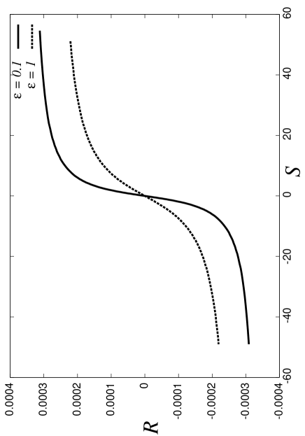
Figure 8: The reward rate $R$ as a function of the skewness $S$ of the skew-normal distribution. The unit of the vertical axis is yen per second. We set the parameters $m$ and $a$ for the Weibull distribution with respect to the first-passage time as $(m,a)=(0.59,50.855)$. We plot it for the cases of $\epsilon=0.1$ and $1$ with $\lambda=-1$.

From this figure, we find that the reward rate increases dramatically as the skewness of the skew-normal distribution (29) becomes positive. As the skewness $S$ increases, the reward rate $R$ saturates at $0.0003$ [yen/s] for our model system, wherein the time interval of the rate change $t$ obeys the Weibull distribution with $(m,a)=(0.59,50.855)$, and the difference of the rate $Y$ follows the skew-normal distribution (29). In this figure, we also find that if we increase the width $\epsilon$ of the rate window from $\epsilon=0.1$ to $1$, the reward rate $R$ decreases. For companies or internet banks, this kind of information might be useful because they can control the reward rate (this takes both positive and negative values) for their customers by tuning the width $\epsilon$ of the rate window in their computer simulations.

Moreover, we should note that we can also evaluate the expected reward $\overline{R}=Rw$, which is the return that the customers can expect to encounter after they log in to their computer systems. By combining the result obtained in this section $R=0.0003$ [yen/s] and the average waiting time $w=42.236\times 60=2534.146$ [s], we conclude that the expected reward should be smaller than $\overline{R}=Rw\,\sim\,0.76$ [yen]. This result seems to be important and useful for both the customers and the bank, e.g. in setting the transaction cost. Of course, the probabilistic model considered here for $P(t)$ or $P(Y)$ is just an example for explaining the stochastic process of the real or empirical rate change. Therefore, several modifications are needed to conduct a much deeper investigation from theoretical viewpoint. Nevertheless, our formulation might be particularly useful in dealing with price changes in real financial markets.

VI Summary and discussion

In this paper, we introduced the concept of queueing theory to analyse price changes in a financial market, for which, we focus on the USD/JPY exchange rate of Sony Bank, which is an internet-based bank. Using the renewal-reward theorem and on the assumption that the Sony Bank rate is described by a first-passage process whose FPT distribution follows a Weibull distribution, we evaluated the average waiting time that Sony Bank customers have to wait until the next rate change after they log in to their computer systems. The theoretical prediction and the result from the empirical data analysis are in good agreement on the value of the average waiting time. Moreover, our analysis revealed that if we assume that the Sony Bank rate is described by a Poisson arrival process with an exponential FPT distribution, the average waiting time predicted by the renewal-reward theorem is half the result predicted by the empirical data analysis. This result justifies the non-exponential time intervals of the Sony Bank USD/JPY exchange rate. We also evaluated the reward that a customer could be expected to encounter by the next price change after they log in to their computer systems. We assumed that the return and FPT follow skew-normal and Weibull distributions, respectively, and found that the expected return for Sony Bank customers is smaller than $\sim\,0.76$ yen. This kind of information about statistical properties might be useful for both the costumers and bank’s system engineers.

As mentioned earlier, in this paper, we applied queueing theoretical analysis to the Sony Bank rate, which is generated as a first-passage process with a rate window of width $2\epsilon$. We did not mention the high-frequency raw data underlying behind the Sony Bank rate because Sony Bank does not record raw data and the data itself is not available to us. Although our results did not suffer from this lack of information, the raw data seems to be attractive and interesting as a material for financial analysis. In particular, the effect of the rate window on high-frequency raw data should be investigated empirically. However, it is impossible for us to conduct such an investigation for the Sony Bank rate. To compensate for this lack of information, we performed the GARCH simulations, wherein the duration between price changes in the raw data obeys a Weibull distribution with parameter $m_{0}$. Next, we investigated the effect of the rate window through the first-passage time distribution under the assumption that it might follow a Weibull distribution with parameter $m\,(\neq m_{0})$. The $m_{0}$-$m$ plot was thus obtained. Nevertheless, an empirical data analysis to investigate the effect might be important. Such a study is beyond the scope of this paper; however, it is possible for us to generate the first-passage process from other high-frequency raw data such as BTP futures. This analysis is currently under way and the results will be reported in our forthcoming article ISE .

As mentioned in TABLE I, the amount of data per day for the Sony Bank rate is about $70$ points, which is less than the tick-by-tick high-frequency data. This is because the Sony Bank rate is generated as a first-passage process of the raw data. This means that the number of data is too few to confirm whether time-varying behaviour is actually observed. In our investigation of the limited data, we found that the first-passage time distribution in a specific time regime (e.g. Monday of each week) obeys a Weibull distribution, but the parameter $m$ is slightly different from $0.59$. However, this result has not yet confirmed because of the low number of data points. Therefore, we used the entire data (about $31,000$ points from September 2002 to May 2004) to determine the Weibull distribution. In this paper, we focused on the evaluation of the average waiting time and achieved the level of accuracy mentioned above. In addition, if Sony Bank records more data in future, we might resolve this issue, namely, whether the Sony Bank rate exhibits time-varying behaviour. This is an important area for future investigation.

Although we dealt with the Sony Bank USD/JPY exchange rate in this paper, our approach is general and applicable to other stochastic processes in financial markets. We hope that it is widely used to evaluate various useful statistics in real markets.

- (1) R.N. Mantegna and H.E. Stanley, An Introduction to Econophysics : Correlations and Complexity in Finance, Cambridge University Press (2000).
- (2) J.-P. Bouchaud and M. Potters, Theory of Financial Risk and Derivative Pricing, Cambridge University Press (2000).
- (3) J. Voit, The Statistical Mechanics of Financial Markets, Springer (2001).
- (4) I. Simonsen, M.H. Jensen and A. Johansen, Eur. Phys. J. B 27, 583 (2002).
- (5) M.H. Jensen, A. Johansen, F. Petroni and I. Simonsen, Physica A 340, 678 (2004).
- (6) M. Raberto, E. Scalas and F. Mainardi, Physica A 314, 749 (2002).
- (7) E. Scalas, R. Gorenflo, H. Luckock, F. Mainardi, M. Mantelli and M. Raberto, Quantitative Finance 4, 695 (2004).
- (8) S. Kurihara, T. Mizuno, H. Takayasu and M. Takayasu, The Application of Econophysics, H. Takayasu (Ed.), pp. 169-173, Springer (2003).
- (9) N. Sazuka, Eur. Phys. J. B 50, 129 (2006).
- (10) N. Sazuka, Physica A 376, 500 (2007).
- (11) D.R. Cox, Renewal Theory, Methuen, London (1961).
- (12) D.R. Cox and V. Isham, Point Processes, Chapman Hall (1981).
- (13) H.C. Tuckwell, Stochastic Processes in the Neuroscience, Society for industrial and applied mathematics, Philadelphia, Pennsylvania (1989).
- (14) W. Gerstner and W. Kistler, Spiking Neuron Models, Cambridge University Press (2002).
- (15) F. Mainardi, M. Raberto, R. Gorenflo and E. Scalas, Physica A 278, 468 (2000).
- (16) R. Gorenflo and F. Mainardi, The asymptotic universality of the Mittag-Leffler waiting time law in continuous random walks, Lecture note at WE-Heraeus-Seminar on Physikzentrum Bad-Honnef (Germany), 12-16 July (2006).
- (17) http://moneykit.net
- (18) S. Redner, A Guide to First-Passage Processes, Cambridge University Press (2001).
- (19) N.G. van Kappen, Stochastic Processes in Physics and Chemistry, North Holland, Amsterdam (1992).
- (20) H. Risken, The Fokker-Planck Equation: Methods of Solution and Applications, Springer-Verlag, Berlin, Heidelberg, New York (1989).
- (21) C.W. Gardiner, Handbook of Stochastic Methods, Springer-Verlag, Berlin, Heidelberg, New York (1983).
- (22) W. Schoutens, Lvy Processes in Finance: Pricing Financial Derivatives, Wiley, New York (2003).
- (23) H.C. Tijms, A first Course in Stochastic Models, John Wiley Sons (2003).
- (24) S. Oishi, Queueing Theory, CORONA PUBLISHING CO., LTD (in Japanese) (2003).
- (25) R.F. Engle, Econometrica 50, 987 (1982).
- (26) T. Ballerslev, Econometrics 31, 307 (1986).
- (27) J. Franke, W. Hrdle and C.M. Hafner, Statistics of Financial Markets : An Introduction, Springer-Verlag, Berlin, Heidelberg, New York(2004).
- (28) B.S. Everitt, The Cambridge Dictionary of Statistics, Cambridge University Press (1998).
- (29) N.T. Chan and C. Shelton, Technical Report AI-MEMO 2001-2005, MIT, AI Lab (2001).
- (30) J. Inoue, N. Sazuka and E. Scalas, in preparation.