An economical method to calculate eigenvalues of the Schrödinger Equation.

Abstract

PACS number

The method is an extension to negative energies of a spectral integral equation method to solve the Schroedinger equation, developed previously for scattering applications. One important innovation is a re-scaling procedure in order to compensate for the exponential behaviour of the negative energy Green’s function. Another is the need to find approximate energy eigenvalues, to serve as starting values for a subsequent iteration procedure. In order to illustrate the new method, the binding energy of the He-He dimer is calculated, using the He-He TTY potential. In view of the small value of the binding energy, the wave function has to be calculated out to a distance of 3000 a.u. Two hundred mesh points were sufficient to obtain an accuracy of three significant figures for the binding energy, and with 320 mesh points the accuracy increased to six significant figures. An application to a potential with two wells, separated by a barrier, is also made.

LABEL:FirstPage1 LABEL:LastPage#1

I Introduction

The much used differential Schrödinger equation is normally solved by means of a finite difference method, such as Numerov or Runge-Kutta, while the equivalent integral Lippmann-Schwinger (LS) equation is rarely solved. The reason, of course, is that the former is easier to implement than the latter. However, a good method for solving the LS equation has recently been developed IEM , and applications to various atomic systems have been presented ESRY , E-H . This method, denoted as S-IEM (for Spectral Integral Equation Method), expands the unknown solution into Chebyshev polynomials, and obtains equations for the respective coefficients. The expansion is called ”spectral”, because it converges very rapidly, and hence is economical in the number of meshpoints required in order to attain a prescribed accuracy. A basic and simple description of the method has now been published CISE , and a MATLAB implementation is also included. However, the applications described so far refer to positive energies, i.e., to scattering situations, while an example for negative energies, i.e., bound states, has up to now not been provided.

Since the solution of many quantum-mechanical problems requires the availability of a basis of discrete negative energy eigenfunctions (or bound states), or of positive energy Sturm-Liouville eigenfunctions, the S-IEM has now been adapted to also obtain eigenfunctions and eigenvalues. Since there are situations where the commonly known eigenvalue-finding methods do not work well, we present here a short description of our method, in the hope that it will be useful for the physics student/teacher community.

An illustration of the method for the case of the bound state of the He-He atomic dimer is presented. This is an interesting case since the binding energy is very small, $1.3\ mK$ or $1.1\times 10^{-7}eV$ , and the corresponding wave function extends out to large distances, between $1000$ to $3000$ atomic units, depending on the accuracy required. Hence a method is desirable that maintains accuracy out to large distances, and that can find small eigenvalues. A commonly used method to obtain eigenvalues consists in discretizing the Schrödinger differential operator into a matrix form, and then numerically obtaining the eigenvalues of this matrix. This procedure gives good accuracy for the low-lying (most bound) eigenvalues, while the least bound eigenvalues become inaccurate. The method described here does not suffer from this difficulty since it finds each eigenvalue of the integral equation iteratively  It also provides a good search procedure for finding initial values of the eigenvalue, required to start the iteration.

II The formalism.

For negative energy eigenvalues the differential equation to be solved is

$$-\frac{\hbar^{2}}{2M}\frac{d^{2}\bar{\psi}}{d\bar{r}^{2}}+(\bar{V}-\bar{E})\bar{\psi}=0$$ (1)

where $\bar{r}$ is the radial distance in units of length, $\bar{V}$ and $\bar{E}$ are the potential energy and the (negative) energy in units of energy, respectively. This is the radial equation for the partial wave of angular momentum $0.$ For atomic physics applications this equation can be written in the dimensionless form

$$-\frac{d^{2}\psi}{dr^{2}}+(V+\kappa^{2})\psi=0$$ (2)

where $r=\bar{r}/a_{0}$ is the relative distance in units of Bohr, and $V$ and $\kappa^{2}$ are given in atomic energy units. The LS eigenvalue equation that is the equivalent to Eq. (2), is

$$\psi(r)=\int_{0}^{T}\mathcal{G}(r,r^{\prime})V(r^{\prime})\psi(r^{\prime})dr^{\prime}$$ (3)

where, as is well known, the Green’s function $\mathcal{G}(r,r^{\prime})$ for negative energies $-\bar{E}=(2M/\hbar^{2})\ \kappa^{2}$ is given by

$$\mathcal{G}(r,r^{\prime})=-\frac{1}{\kappa}F(r_{<})G(r_{>}^{\prime})$$ (4)

$r_{<}$ and $r_{>}$ being the lesser and larger values of $r$ and $r^{\prime}$, respectively, and

$$F(r)=\sinh(\kappa r),\ \ \ \ \ G(r)=\exp(-\kappa r).$$ (5)

The Eq. (3) is a Fredholm integral eigenvalue equation of the first kind. Unless the wave number $\kappa$ has a correct value, the solution does not satisfy the boundary condition that $\psi(r)$ decay exponentially at large distances. As shown by Hartree many years ago, a method of finding a correct value of $\kappa$ is to start with an initial guess $\kappa_{s}$ for $\kappa$, divide the corresponding (wrong) wave function into an ”out” and and ”in” part, and match the two at an intermediary point $T_{M}$. The $out$ part $\psi_{O}$ is obtained by integrating (3) from the origin to an intermediate radial distance $T_{M}$, and $\psi_{I}$ is the result of integrating (3) from the upper limit of the radial range $T$ inward to $T_{M}$. For the present application the integration method is based on the S-IEM, described in Appendix 1. The function $\psi_{0}$ is renormalized so as to be equal to $\psi_{I}$ at $r=T_{M}$ and its value at $r=T_{M}$ is denoted as $\psi_{M}$. The derivatives with respect to $r$ at $r=T_{M}$ are calculated, as described in Appendix 1, and are denoted as $\psi_{0}^{\prime}$ and $\psi_{I}^{\prime}$, respectively. The new value of the wave number $\kappa_{s+1}$ is given in terms of these quantities as

$$\kappa_{s+1}=\kappa_{s}-(Iter)_{s}$$ (6)

where

$$(Iter)_{s}=\frac{1}{2\kappa_{s}}\frac{\psi_{M}(\psi_{0}^{\prime}-\psi_{I}^{\prime})_{M}}{\int_{0}^{T_{M}}\psi_{0}^{2}dr+\int_{T_{M}}^{T}\psi_{I}^{2}dr}$$ (7)

Equations (6) and (7) can be derived by first writing (2) for the exact wave function $\psi_{E}$ (using $\kappa_{\infty}$ for $\kappa_{s}$ and (2) for the approximate wave function $\psi_{A}=(\psi_{0}$ or $\psi_{I})$, multiplying each equation by the other wave function, integrating over $r$, and subtracting one from another. When $\kappa_{\infty}$ is replaced by $\kappa_{s+1}$ and $\psi_{E}$ is replaced by $\psi_{A}$ then equations (6) and (7) result.

III The Spectral Method

The S-IEM procedure to evaluate $\psi_{0}$ and $\psi_{I}$ is as follows. First the whole radial interval $0\leq r\leq T$ is divided into $m$ partitions, with the $i$-th partition defined as $t_{i-1}\leq r\leq t_{i}$, $i=1,2,\cdots m$. For notational convenience we denote the $i$-th partition simply as $i$. In each partition $i$ two independent functions $y_{i}(r)$ and $z_{i}(r)$ are obtained by solving the integral equations

$$y_{i}(r)=\int_{t_{i-1}}^{t_{i}}\mathcal{G}(r,r^{\prime})V(r^{\prime})y_{i}(r^{\prime})dr^{\prime}+f_{i}(r)$$ (8)

and

$$z_{i}(r)=\int_{t_{i-1}}^{t_{i}}\mathcal{G}(r,r^{\prime})V(r^{\prime})z_{i}(r^{\prime})dr^{\prime}+g_{i}(r).$$ (9)

Here $f_{i}$ and $g_{i}$ are scaled forms of the functions $F$ and $G$ defined above on the interval $i$,

$$f_{i}(r)=\sinh(\kappa r)\times E_{i},~{}~{}~{}~{}g_{i}(r)=\exp(-\kappa r)/E_{i},$$ (10)

and the scaling factor $E_{i}$ in each partition $i$ is given by

$$E_{i}=\exp(-\kappa t_{i}).$$ (11)

Such scaling factors are needed in order to prevent the unscaled functions $\sinh(\kappa r)$ and $\exp(-\kappa r),$ and the corresponding functions $Y_{i}$ and $Z_{i}$ to become too disparate at large distances, which in turn would result in a loss of accuracy. Apart from these scaling operations, the calculation of functions $y_{i}$ and $z_{i}$ by means of expansions into Chebychev polynomials, as well as the determination of the size of the partition $i$ in terms of the tolerance parameter $\varepsilon$ is very similar to the calculation of the functions $Y_{i}$ and $Z_{i}$ described in Ref. (CISE ). The number of Chebychev polynomials in each partition is normally taken as $N=16$. The equations (8) and (9) are Fredholm integral equation of the 2nd kind, and hence are much easier to solve than the Fredholm equations of the first kind.

The global wave function $\psi$ is given in each partition by

$$\psi(r)=a_{i}y_{i}(r)+b_{i}z_{i}(r).$$ (12)

In order to obtain the coefficients $a_{i}$ and $b_{i}$ for each partitions $i$ one proceeds similarly to ”Method B” described in Ref. (CISE ), that relates these coefficients from one partition to those in a neighboring partition. That relation is

$$\left[\begin{array}[c]{cc}E_{i}/E_{i+1}&0\\ 0&E_{i+1}/E_{i}\end{array}\right]\omega_{i+1}\left[\begin{array}[c]{c}a_{i+1}\\ b_{i+1}\end{array}\right]=\gamma_{i}\left[\begin{array}[c]{c}a_{i}\\ b_{i}\end{array}\right],$$ (13)

where the elements of the $2\times 2$ matrices $\omega$ and $\gamma$ are given in terms of overlap integrals $\left\langle fy\right\rangle_{i},$ $\left\langle fz\right\rangle_{i},$ $\left\langle gy\right\rangle_{i},$ $\left\langle gz\right\rangle_{i},$ of the type $\left\langle fy\right\rangle_{i}=\int_{t_{i-1}}^{t_{i}}f_{i}(r)V(r)y_{i}(r)dr$, as is described in further detail in the Appendix 1. This relation enables one to march outward by obtaining $a_{O,i+1}$ and $b_{O,i+1}$ in terms of $a_{O,i}$ and $b_{O,i},$ and inward by obtaining $a_{I,i}$ and $b_{I,i}$ in terms of $a_{I,i+1}$ and $b_{I,i+1}.$The integration outward is started at the innermost partition $i=1$ with $a_{O,1}=1/E_{1},$ and the integration inwards is started at the outermost partition (ending at T), for which the coefficients $a_{m}$ and $b_{m}$ are given as $0$ and $E_{m},$ respectively. The values of the functions $I$ and $O$ and their derivatives at the inner matching point $T_{M}$, as well as the integrals $\int_{0}^{T_{M}}\psi_{O}^{2}dr+\int_{T_{M}}^{T}\psi_{I}^{2}dr,$ required for evaluating $Iter$ in Eq. (7), can be obtained in terms of the overlap integrals described above, as is described in Appendix 1. The iteration for the final value of $\kappa$ proceeds until the value of $Iter$ is smaller than a prescribed tolerance. The important question of how to find an initial value $\kappa_{0}$ of $\kappa$ is described in the next section.

IV Search for the initial values of $\kappa$

Since the present method does not obtain all the values of the energy as the eigenvalues of one big matrix, but rather obtains iteratively one selected eigenvalue at a time, it is necessary to have a reliable algorithm for finding the appropriate starting values $\kappa_{0}$ for the iteration procedure.

The present search method is based on Eq. (12), according to which the solution $\psi$ in a given partition $i$ is made up of two parts, $y_{i}(r)$ and $z_{i}(r).$ In the radial regions where the potential is small compared to the energy, i.e., in the ”far” region beyond the outer turning point, the functions $y_{i}(r)$ and $z_{i}(r)$ are nearly equal to the driving terms $f$ and $g$ of the respective integral equations (8) and (9). Hence, for negative energies, according to Eqs. (10),  in the ”far” region $y_{i}(r)$ has an exponentially increasing behavior, while $z_{i}(r)$ is exponentially decreasing. For the correct bound state energy eigenvalue the solution $\psi$ has to decrease exponentially at large distances, and hence the coefficient $a_{i}$  in Eq. (12) has to be zero for the last partition $i=m$. Hence, as a function of $\kappa$ the coefficient $a_{m}$ goes through zero at a value of $\kappa$ equal to one of the the bound state energies.

Based on the above considerations, the search procedure for the initial value $\kappa_{0}$ is as follows: A convenient grid of equispaced $\kappa_{s}$ values is constructed, $s=1,2,...$ and for each $\kappa_{s}$ the integration  ”outward” for the wave function is carried out to $T_{M}\lesssim T$ , but $Iter$ is not calculated. The value of $T_{M}$ is selected such that the potential $V$ is less than the expected binding energy. The values of the coefficient $a_{O,i_{M}}$ for the last partition $i_{M}$ are recorded, and the values of $\kappa_{s}$ for which $a_{O,i_{M}}$ changes sign are the desired starting values $\kappa_{0}$ for the iteration procedure. The numerical example, given in the sections describing the calculation of the $He-He$ bound state, shows that this search method is very reliable.

IV.1 The Numerical Code

The code was written in MATLAB, and is available from the authors both in MATLAB and in FORTRAN versions. The code that performs the iterations is denoted as $Iter\_neg\_k,$ and the search code for finding the starting values $\kappa_{0}$ is denoted as $Searchab\_neg\_k.$ The subroutines for both codes are the same. The validity of the code was tested by comparing the resulting binding energy with a non-iterative spectral algorithm that obtains the eigenvalues of a matrix. The potential used for this comparison was an analytical approximation to the $He-He$ potential $TTY$ TTY , described in the next section. The comparison algorithm expands the wave function from $R_{START}$ to $T$ (no partitions) in terms of scaled Legendre polynomials up to order $N$. The operator $-d^{2}/dr^{2}+V$ is discretized into a matrix at zeros of the Legendre polynomial of order $N+1$. The boundary conditions that the wave function vanishes at both $R_{START}$ and at $T$ are incorporated into the matrix, and the eigenvalues of the matrix are calculated. The agreement between the two codes for the binding energy was good to 6 significant figures.

In the test-calculation for the $He-He$ dimer binding energy described below, the convergence rate of the iterations, the stability with respect to the value of a repulsive core cut-off parameter, and also the number of mesh-points required for a given input value of the tolerance parameter will be examined. A bench-mark calculation of the dimer binding energy is also provided for students that would like to compare their method of calculation to ours. In these calculations the TTY potential is replaced by an analytical approximation that is easier to implement.

V Application to the $He-He$ dimer

The He-He dimer is an interesting molecule, because, being so weakly bound, it is the largest two-atom molecule known. The He-He interaction, although weak, does influence properties such as the superfluidity of bulk He II, of He clusters, the formation of Bose-Einstein condensates, and the calculation of the He trimer. In 1982 Stwalley et al STWALLEY were the first to conjecture the existence of a He-He dimer. The first experimental indication of the dimer’s existence was found in 1993 LUO , and since 1994 it was explored by means of a series of beautiful diffraction experiments. Through these diffraction experiments not only has the existence of the dimer, but also that of the trimer, been unequivocally demonstrated and an indication of the spatial extent of these molecules has also been obtained SCHOEL , Grisenti , BRUHL . Various precise calculations of the He-He interaction have subsequently been performed THEO and the corresponding theoretical binding energies of the dimer (close to $1.3\ mK\approx 1.1\times 10^{-7}eV$, see Table 1 in Ref. SANDH ) and the trimer (the ground state of the trimer is close to $126mK$, see for instance Ref. SOFIANOS ) agree with experiment to within the experimental uncertainty. The wave function of the He dimer or trimer extends out to large distances (several thousand atomic units), the binding energy is very weak, and the transition from the region of the large repulsive core to the weak attractive potential valley is very abrupt. For these reasons the dimer (or trimer) calculations involving He atoms require good numerical accuracy, and therefore was chosen as a test case for our new algorithm.

The transition from Eq. (1) to the dimensionless Eq. (2), is accomplished by transforming the potential and the energy into dimensionless quantities as follows

$$V=Q\bar{V}$$ (14)

$$\kappa^{2}=-Q\bar{E}$$ (15)

where $Q$ is a normalization constant, defined in Appendix 2. For the case of two colliding $He$ atoms interacting via the $TTY$ potential we take the mass of the He atom as given in Ref. SANDH , for which the value of $Q$ is $7295.8356.$ For the calculations involving our analytical fits to the $TTY$ potential, we take for $Q$ the value $7296.3.$

The $TTY$ potential TTY , and one analytic fit, are shown in Fig. (1). The repulsive core goes out to about $5\ a_{0}$ and the

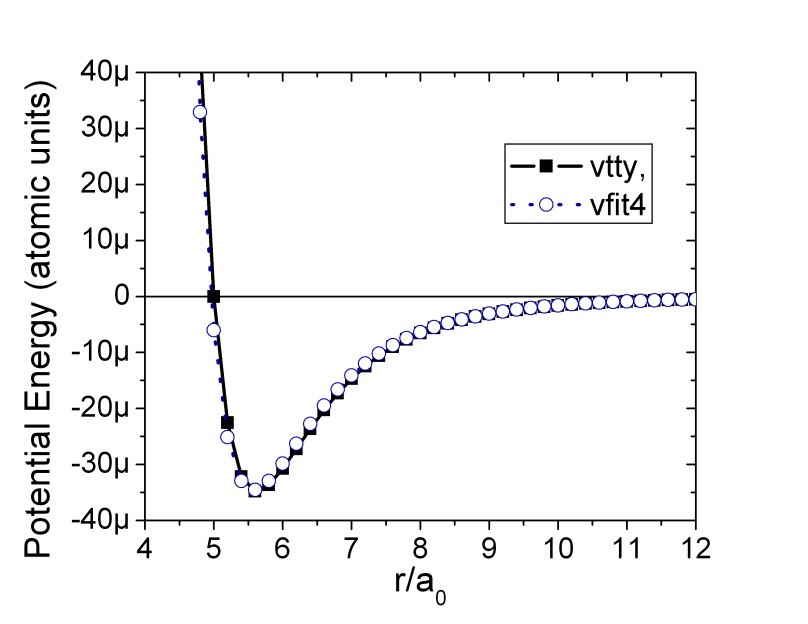
Figure 1: The ”TTY” He-He potential given by Tang, Toennies, and Yiu TTY , and the fit FIT 4 , as a function of distance.

subsequent attractive valley reaches its maximum depth of $3.5\times 10^{-5}au$ (approximately $10^{-3}eV$) near $r\simeq 5.6\ a_{0}$. This attractive potential valley then decays slowly over large distances approximately like $r^{-6}$. The corresponding energy of the bound state is $\simeq-10^{-7}ev$ TTY . In the units defined in $(\ref{schr2})$ the potential valley has a depth of $0.26$ and the binding energy has the value of $3.04\times 10^{-5}$. The bound state wave function peaks near $r=10\ a_{0}$ and decays slowly from there on. The outer turning point occurs near $30\ a_{0}$; the value of the wave function at $r=2500\ a_{0}$ is $\simeq 10^{-7}$, and at $3000\ a_{0}$ it is $\simeq 6\times 10^{-9}$. The quantity $r\times\psi^{2}\ \$has its maximum beyond the turning point near $r=100\ a_{0}$, and the average radial separation $\left\langle r\right\rangle=\int_{0}^{\infty}\psi^{2}\ r\ dr$ is close to $\simeq 97\ a_{0}.$

V.1 Results for the $TTY$ Potential

The $TTY$ He-He potential is calculated by means of Fortran code provided by Franco Gianturco Franco , and modified at hoc for small distances (less than $1\ a_{0}$) so that it maintains the repulsive core nature. The potential is ”cut off” at a distance $R_{cut}$ so that for $r\leq R_{cut}$, $V(r)=V(R_{cut})$. The S-IEM calculation starts at $r=0$ and extends to $T=3,000$ $a_{0.}$ The intermediary matching point is $T_{M}=7\ a_{0}$. The dependence of the eigenvalue on $R_{cut},$ and the rate of convergence of the iterations, are described in Appendix 3. Our choice for the value of $R_{cut}=2.5\ a_{0}$, of $T=3,000$, and of the tolerance parameter $\varepsilon=10^{-12}$ is such that the numerical stability of our results is better than $12$ significant figures.

Our value for the binding energy is compared with that of other calculations in Table 1.

	$B.E.(mK)$	$<r>(nm)$
Present	$\mathbf{1.31461}$	$\mathbf{5.1607}$
Ref. SANDH	$\mathbf{1.30962}$
Ref. TTY	$\mathbf{1.316}$
Experiment Grisenti	$\mathbf{0.9-1.4}$	$\mathbf{5.2\pm 0.4}$

Table 1: Comparison of the He-He Binding Energies obtained by various authors.

. The comparison shows good agreement of our result with the literature. The difference between our S-IEM result and that of Ref. SANDH could well be due to a slightly different choice of the parameters that determine $TTY.$

V.2 Numerical Properties of the S-IEM.

In order to examine the nature of the partition distribution and the resulting accuracy as a function of the tolerance parameter $\varepsilon$ and also in order to provide a bench-mark calculation, the $TTY$ potential was replaced by an analytical approximation defined in the equation below.

$$V(r) =p_{1}\exp(-(r-p_{2})/p_{3})\times\left[2-\exp(-(r-p_{2})/p_{3})\right]$$

$$-p_{6}\times(r^{-5.807})/\left\{1+\exp\left[-p_{5}(r-p_{4})\right]\right\}.$$ (16)

The parameters $p_{1}$ to $p_{6}$ for two fits, denoted FIT 3 and FIT 4, are given in Table 2. The resulting potential is in atomic units; $r,p_{2},p_{3}$ and $p_{4}$ are in units of $a_{0}$; $p_{5}$ is in units of $a_{0}^{-1}$ and $p_{1}$ and $p_{6}$ are in atomic energy units. For all calculations involving these analytical fits, $Q$ defined in Eq. (14), has the value $7296.3.$

parameters	FIT 3	FIT 4
$p_{1}$	-3.4401e-5	-2.930 e-5
$p_{2}$	5.606	5.590
$p_{3}$	0.8695	0.8511
$p_{4}$	7.657	7.5892
$p_{5}$	1.750	0.95608
$p_{6}$	0.6784	0.89098

Table 2: Parameters for two analytic fits to the TTY potential

Fits 3 (4) produce a more (less) repulsive core than TTY, and is more (less) attractive in the region of the potential minimum.

Our algorithm automatically chooses the size of the partitions such that the error in the functions calculated in each partition does not exceed the tolerance parameter $\varepsilon.$ At small distances the density of partitions is very high, but beyond $500\ a_{0}$ the size of the partitions increase to about $440\ a_{0}$. In the region near the repulsive core the partitions are approximately $0.5$ $a_{0}$ wide, but there is a region in the vicinity of $R_{cut\text{ }}$ where they crowd together much more. The latter is illustrated in Fig. (2) for FIT 4, for $R_{cut}=2.5\ a_{0},$ for various values of the tolerance parameter $\varepsilon$. In Table 3 the corresponding accuracy of the binding energy is displayed, for the case that the $He-He$ potential energy is given by Fit 4. It is noteworthy that the number of reliable significant figures in $\kappa$ tracks faithfully the value of the tolerance parameter, as is shown in Table 3.

Figure 2: Partition distribution in the radial region up to 4 $a_{0}$ for three different values of the tolerance parameter. The value of the latter is listed in the legend and in Table 3. The potential is given by FIT 4, described in the text and the value of $R_{cut}=2.5\ a_{0}.$ The total number of partitions for each case is given by the numbers near the curves.

$Tol$	$\kappa\times 10^{3}~{}(a_{0})^{-1}$	$M$	$No.\ of\ Meshpts$
$10^{-12}$	$5.0817542$	$47$	$652$
$10^{-6}$	$5.0817461$	$19$	$275$
$10^{-3}$	$5.0776$	$13$	$208$

Table 3: Accuracy of the wave number (it is the square root of the binding energy) as a function of the tolerance parameter. The total number of partitions for each case is denoted by M. The corresponding partition distributions are displayed in Fig. 4

V.3 The Search for the Starting Values $\kappa_{0}.$

An example of the search procedure is given in Table 4, for a potential given by Fit 4, Eq. (16), multiplied by the factor $\lambda=$ $20$. The mesh of $\kappa$ values starts at $\kappa=-2\$and proceeds by steps of $\Delta\kappa=0.05$ until $\kappa=-0.05$ (all in units of $a_{0}^{-1}$). The mesh values of $\kappa$ for which the coefficient $a_{m}$ of $y_{m}(r)$ changes sign are shown in the first column of Table 4, and the corresponding iterated value of $\kappa$ is shown in the third column. The value of $T_{M}=80\ a.u.$, and $iter=10^{-6}$. The MATLAB computing time required for carrying out the $40$ mesh search calculations is $3.8\ s$ on a $2$ GHz PC; the approximately $7$ iterations required for obtaining the more precise values of each $\kappa$ shown in the third column take approximately $1\ s.$ of computer time.

$\kappa-Mesh$	sign of $a_{m}$	$\kappa-Iterated$	# of nodes
$1.70$	$+\rightarrow-$	$1.7028$	$0$
$0.70$	$-\rightarrow+$	$0.7273$	$1$
$0.05$	$+\rightarrow-$	$0.0561$	$2$

Table 4: Search of the wave number eigenvalues for a He-He Fit 4 potential multiplied by 20

.
By repeating the same procedure for different values of $\lambda$, one can trace the $\kappa$ eigenvalues down to $\lambda=1.$

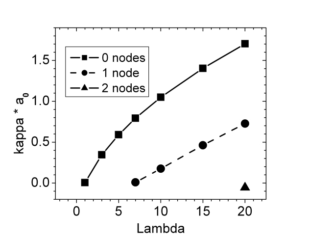
Figure 3: The eigenvalues of $\kappa$ as a function of the strength parameter $\lambda$ of the Fit 4 Potential.

The result, displayed in Fig. (3), shows that the values of $\kappa$ depend nearly linearly on the value of $\lambda.$ Futher searches with values of $\lambda$ slightly less than unity showed that the code was able to find an energy that is approximately 25 times less bound than the result for the $TTY$ potential.

In order to provide a benchmark calculation, the values of $\kappa$ obtained with the potential of FIT 4 are listed in Table 5. The value of $Q$ is $7296.3$, the values of $T_{M}$ and $T$ are $7$ and $3,000\ a_{0},$ respectively, and $\lambda=1.0$

$R_{cut}~{}(a_{0})$	$\kappa~{}(a_{0})^{-1}$
2.5	5.08175419E-3
3.0	5.08176556E-3
3.5	5.10608688E-3

Table 5: The values of the bound state wave number for potential of FIT 4, for various values of the cut-off radius . Additional information is given in the text

VI Application to a double well potential.

The case for which the potential has two (or more) wells separated by one (or more) barriers offers another test for the reliability and accuracy of a numerical procedure for obtaining eigenvalues of the Schrödinger equation. The reason is that the energy eigenvalues are split by a small amount, corresponding to the situation in which the wave function located in one of the wells has either the same or the opposite sign of the wave function located in the adjoining well. The larger the barrier, the smaller is the difference $\Delta E$ between the two energies, and the larger are the demands on the numerical procedure. An interesting relaxation method for finding energy eigenvalues contained in a prescribed interval has been described in Ref. Carlo . The double well potential, in the units of Eq. (2) is

$$V=-\Lambda x^{2}+x^{4},\text{~{}~{}}-T_{m}\leq x\leq T_{m}.$$ (17)

The value of $\Delta E$ for the difference between the two lowest eigenvalues were calculated here by using the S-IEM method described in this paper, denoted as $(\Delta E)_{IEM}$and also by a matrix eigenvalue method, denoted as $(\Delta E)_{L}.$ This method discretizes the Schrödinger operator on the left hand side of Eq. (18)

$$(-\frac{d^{2}}{dr^{2}}+V)\psi=E\ \psi$$ (18)

at the zeros of a Legendre Polynomial of order $n_{L},$ and then finds all the eigenvalues of the corresponding matrix using the standard QR algorithm. The comparison of the results for the three largest values of $\Lambda$ is shown in Table 6, where $(\Delta E)_{rel}$ denotes the result obtained in Ref. Carlo

$\Lambda$	$(\Delta E)_{IEM}$	$(\Delta E)_{L}$	$(\Delta E)_{rel}$
$10$	3.02E-5	2.98185E-5	2.9821E-5
$12$	3.53E-7	3.508E-7	3.5093E-7
$15$	2E-10	2E-10	1.9499E-10

Table 6: Comparison between three different methods of calculating energy eigenvalues. The table shows the difference between the two lowest eigenvalues of the double well potential defined in this section

For the S-IEM the value of the tolerance parameter was $\varepsilon=10^{-12},$ and the corresponding accuracy was sufficient to obtain the results shown in the Table 6. However, it can be seen that the relaxation method is more accurate than the S-IEM method. The difference between the results in Table 6 could well be due to differences in the choice of the value of $T_{M}$. For the $(\Delta E)_{L}$ result, the value of $T_{M}$ was varied between $6$ and $9$ units of length, and the number of Legendre polynomials $n_{L}$ was varied between $200$ and $700.$ The numerical stability of the QR algorithm is well documented in the numerical linear algebra literature. The convergence of the Legendre discretization of the Schrödinger operator using finite series expansions in orthogonal polynomials, such as Legendre, Chebyshev and others, is also well understood, as discussed for example in Ref IEM .

VII Summary and Conclusions.

An integral equation method (S-IEM) IEM for solving the Schrödinger equation for positive energies has been extended to negative bound-state energy eigenvalues. Our new algorithm is in principle very similar to an iterative method given by Hartree in 1930, in that it guesses a binding energy, integrates the Schrödinger Equation inwards to an intermediary matching point starting at a large distance, integrates it outwards from a small distance to the same matching point, and from the difference between the logarithmic derivatives at this point an improved value of the energy is found. Our main innovation to this scheme is to replace the usual finite difference method of solving the Schrödinger equation by a method which solves the corresponding integral (Lippman-Schwinger) equation. That method expands the wave function in each radial partition in terms of Chebyshev polynomials, and solves matrix equations for the coefficients of the expansion. Increased accuracy is obtained by this procedure for three reasons: a) the solution of an integral equation is inherently more accurate than the solution of a differential equation; b) by using integral equations, the derivatives of the wave function required at the internal matching points can be expressed in terms of integrals that are more accurate than calculating the derivatives by a numerical three- or five point formula, and c) because of the spectral nature of the expansion of the wave function in each partition, the length of each partition can be automatically adjusted in order to maintain a prescribed accuracy. This last property enables the S-IEM to treat accurately the abrupt transition of the wave function from the repulsive core region into the attractive valley region. This feature, once applied to the solution of the three-body problem, is also of importance in the exploration of the Efimov states INCAO .

To illustrate this method, the binding energy of the He dimer has been calculated, based on the $TTY$ potential given by Tang, Toennies, and Yiu TTY . The result is close to the ones quoted in the literature, as displayed in Table 7. Additional numerical properties of the S-IEM have been explored by means of the $He-He$ example. The accuracy of the binding energy was found to faithfully track the input value of the tolerance parameter, as is shown in Table 3. The meshpoint economy of the method is very good. For an accuracy of three significant figures, the number of meshpoints needed in the radial interval between $0$ and $3,000\ a.u.$ required only $208$ mesh points. After an addition of $70$ meshpoints, the accuracy increased to six significant figures.

One of the authors (GR) acknowledges useful conversations with F. A. Gianturco, W. Glöckle, I. Simbotin, W. C. Stwalley, and K. T. Tang

Appendix 1: Recursion Relations for the coefficients ${\LARGE a}$and ${\LARGE b}$.

The recursion relation between coefficients $a$  and $b$ , from one partition to a neighbouring partition is given by Eq. (13) in the text. The corresponding matrices $\omega_{i}$ and $\gamma_{i}$ are given by

$$\omega_{i}=\left[\begin{array}[c]{cc}0&1\\ 1-\left\langle gy\right\rangle_{i}&-\left\langle gz\right\rangle_{i}\end{array}\right]$$ (19)

$$\gamma_{i}=\left[\begin{array}[c]{cc}-\left\langle fy\right\rangle_{i}&1-\left\langle fz\right\rangle_{i}\\ 1&0\end{array}\right]$$ (20)

where

$$\left\langle fy\right\rangle_{i}=\int_{t_{i-1}}^{t_{i}}f_{i}(r)V(r)y_{i}(r)dr$$ (21)

$$\left\langle fz\right\rangle_{i}=\int_{t_{i-1}}^{t_{i}}f_{i}(r)V(r)z_{i}(r)dr$$ (22)

$$\left\langle gy\right\rangle_{i}=\int_{t_{i-1}}^{t_{i}}g_{i}(r)V(r)y_{i}(r)dr$$ (23)

$$\left\langle gz\right\rangle_{i}=\int_{t_{i-1}}^{t_{i}}g_{i}(r)V(r)z_{i}(r)dr.$$ (24)

Equation (13) enables one to march outward

$$\left[\begin{array}[c]{c}a_{0,i+1}\\ b_{0,i+1}\end{array}\right]=(\omega_{i+1})^{-1}\left[\begin{array}[c]{cc}E_{i+1}/E_{i}&0\\ 0&E_{i}/E_{i+1}\end{array}\right]\gamma_{i}\left[\begin{array}[c]{c}a_{0,i}\\ b_{0,i}\end{array}\right],$$ (25)

or inward

$$\left[\begin{array}[c]{c}a_{I,i}\\ b_{I,i}\end{array}\right]=\gamma_{i}^{-1}\left[\begin{array}[c]{cc}E_{i}/E_{i+1}&0\\ 0&E_{i+1}/E_{i}\end{array}\right]\omega_{i+1}\left[\begin{array}[c]{c}a_{I,i+1}\\ b_{I,i+1}\end{array}\right].$$ (26)

The integration outward is started at the innermost partition $i=1$ with

$$\left[\begin{array}[c]{c}a_{O,1}\\ b_{O,1}\end{array}\right]=\left[\begin{array}[c]{c}1/E_{1}\\ 0\end{array}\right],$$ (27)

and the integration inwards is started at the outermost partition (ending at T), for which the coefficients $a_{m}$ and $b_{m}$ are given as

$$\left[\begin{array}[c]{c}a_{I,m}\\ b_{I,m}\end{array}\right]=\left[\begin{array}[c]{c}0\\ E_{m}\end{array}\right].$$ (28)

If the calculation of positive energy Sturm-Liouville functions is envisaged, whose asymptotic behavior is $\exp(ikr)$ and approach $0$ for $r\rightarrow 0,$ then $a_{I,m}=i$ and $b_{I,m}=1,$ while $a_{O,1}=1$ and $b_{O,1}=0$

The values of the functions $y$ and $z$ and their derivatives at upper and lower end-points $t_{i}$ and $t_{i-1}$ of partition $i,$ required in the evaluation of Eq. (7), are obtained from integral equations that these functions obey. The result is CISE

$$y_{i}(t_{i})=f_{i}(t_{i})-\left\langle fy\right\rangle_{i}g_{i}(t_{i}),$$ (29)

$$z_{i}(t_{i})=g_{i}(t_{i})(1-\left\langle fz\right\rangle_{i}),$$ (30)

$$y_{i}(t_{i-1})=f_{i}(t_{i-1})(1-\left\langle gy\right\rangle_{i}),$$ (31)

$$z_{i}(t_{i-1})=g_{i}(t_{i-1})-f_{i}(t_{i-1})\left\langle gz\right\rangle_{i}.$$ (32)

Expressions for the derivatives of $y$ and $z$ at upper and lower end-points $t_{i}$ and $t_{i-1}$ of partition $i$ are obtained by replacing functions $f$ and $g$ by their respective derivatives in the above equations. Since derivatives of the functions $f$ and $g$ are given analytically, the values of the derivatives of $y$ and $z$ at the end-points are obtained without loss of accuracy, contrary to what is the case when finite difference methods are employed

Appendix 2: Units

The transition from Eq. (1) to the dimensionless Eq. (2) is accomplished by transforming the potential and the energy into dimensionless quantities according to Eqs. (14) and (15). The normalization constant is given by

$$Q=\frac{2M}{\hbar^{2}}a_{0}^{2}\times 2\mathbb{R}=\frac{2M}{m_{e}},$$ (33)

where $a_{0}$ is the Bohr radius, $2\mathbb{R}$ is the atomic energy unit ($\mathbb{R\simeq}13.606eV$), $\hbar$ is Plank’s constant divided by $2\pi$, $M$ is the reduced mass of the colliding atoms , and $m_{e}$ is the mass of the electron.

For the case of two colliding He atoms interacting via the $TTY$ potential we take the mass of the $He$ atom as given in Ref. SANDH , i.e., $\hbar^{2}/M_{{}^{4}He}=12.12\ K\ \mathring{A}^{2}$ for which the value of $Q$ is

$$Q=7295.8356$$ (34)

Once $\kappa^{2}$ is obtained as the eigenvalue of equation (2), then the corresponding value of $\bar{E}$ in units of $eV$ is given by

$$\bar{E}=-\frac{\kappa^{2}}{Q}\times(27.211396)\ \ eV$$ (35)

It is also useful to express the energy in units of the Boltzman constant, denoted by $K$ in atomic language. In this case $\bar{E}$ is given as

$$\bar{E}=-\frac{\kappa^{2}}{Q}\times\frac{27.211396}{8.617385\times 10^{-5}}\ \ K.$$ (36)

Appendix 3: Accuracy Considerations

The quantities required for Eqs. (25) and (26) are known to the same accuracy as the functions $y$ and $z$ in each partitions, given by the value of the tolerance parameter $\varepsilon$. The propagation of the coefficients $a_{i}$ and $b_{i}$ across the partitions involves as many matrix inversions and multiplications in Eqs. (25) and 26) as there are partitions, and thus the accuracy of $\kappa_{s}$  for each iteration, given by Eq. (7), is reduced by $tol\times$ number of partitions. The number of partitions is approximately $30$, hence for $\varepsilon=10^{-12}$ the accuracy of the final wave number eigenvalue $\kappa$ is expected to be better than $10^{-10}$.

The rate of convergence of the iterations is shown in Table 7.

$s$	$\kappa_{s}$  ($a_{0}$)-1	$Iter_{s}$ (from (7))
$0$	$\mathbf{3}.0\ E-3$	$-2.5002592843\ E-3$
$1$	$\mathbf{5.5}002592823\ E-3$	$-1.0967998971\ E-5$
$2$	$\mathbf{5.511227}2813\ E-3$	$-2.0105203008\ E-10$
$3$	$\mathbf{5.5112274823\ }E-3$	$-4.9700035857\ E-16$

Table 7: Convergence of the iterations for the wave number . The quantitie after the letter E denote the powers of 10 by which the quantities are to be multiplied.

. The sensitivity of the binding energy to the values of $R_{cut}$ is given in Table 8.

$R_{cut}(a_{0})$	$B.E.(m.K)$	$<r>(a_{0})$
$2.0$	$\mathbf{1.3146101}$	$\mathbf{97.7419}$
$2.5$	$\mathbf{1.3146101}$	$\mathbf{97.7419}$
$3.0$	$\mathbf{1.3146143}$	$\mathbf{97.7418}$
$3.5$	$\mathbf{1.3219315}$	$\mathbf{97.4935}$

Table 8: Sensitivity of the He-He Binding Energy to the value of the cuting-off radius $R_{cut}$

.  The table shows that the repulsive core has a non-negligible effect in the $7th$ significant figure beyond $2.5\ a_{0}$.

References

- (1) R. A. Gonzales, J. Eisert, I Koltracht, M. Neumann and G. Rawitscher, J. of Comput. Phys. 134, 134-149 (1997); R. A. Gonzales, S.-Y. Kang, I. Koltracht and G. Rawitscher, J. of Comput. Phys. 153, 160-202 (1999);
- (2) G.H. Rawitscher et al., “Comparison of Numerical Methods for the Calculation of Cold Atom Collisions,” J Chemical Physics, vol. 111, 10418 (1999);
- (3) G.H. Rawitscher, S.-Y. Kang, and I. Koltracht, “A Novel Method for the Solution of the Schrodinger Equation in the Presence of Exchange Terms,” J. Chemical Physics, 118, 9149 (2003);
- (4) G. Rawitscher and I. Koltracht, Computing in. Sc. and Eng., 7, 58 (2005);
- (5) Yea-Hwang Uang and William C. Stwalley, The possibility of a bound state, effective range theory, and very low energy He_He scattering, J. Chem Phys 76 (10) 5069 (1982);
- (6) F. Luo, G. C. McBane, G. Kim, C. F. Giese and W. R. Gentry, J. Chem. Phys. 98, 3564 (1993);
- (7) W. Schöllkopf and J. P. Toennies, Science 266, 1345 (1994);
- (8) R. E. Grisenti, W. Schöllkopf and J. P. Toennies, Phys. Rev. Lett. 85, 2284(2000);
- (9) R. Bruhl, A. Kalinin, O. Kornilov, J. P. Toennies, G. C. Hegerfeldt, and M. Stoll, Phys. Rev. Lett. 95, 063002 (2005);
- (10) R. A. Aziz, F. R. W. McCount, and C. C. Wong, Mol. Phys. 61, 1987 (1987); R. A. Aziz and M. J. Slaman, J. Chem. Phys. 94, 8047 (1991), A. R. Janzen and R. A. Aziz, J. Chem. Phys. 107, 914 (1997); James B. Anderson, J. Chem. Phys. 120, 9886 (2004);
- (11) Elena A. Kolganova, Alexander K. Motovilov, and Werner Sandhas, Phys. Rev. A 70, 052711 (2004);
- (12) A.K. Motovilov, W. Sandhas, S.A. Sofianos, E.A. Kolganova, Eur. Phys. J. D 13, 33 (2001);
- (13) K. T. Tang, J. P. Toennies, and C. L. Yiu, Phys. Rev. Lett. 74, 1546 (1995);
- (14) The authors thank Professor Franco A. Gianturco, from the University of Rome ”La Sapienza” for stimulating conversations and for permission to use his Fortran code;
- (15) C. Presilla and U. Tambini, Phys. Rev. E 52, 4495 (1995);
- (16) J. P. D’Incao and B. D. Esry, Phys. Rev. A 72, 032710 (2005); Eric Braaten and H.-W. Hammer, Physics Reports, 428, # 5-6, 259 (2006).