Football fever: goal distributions and non-Gaussian statistics

Abstract

Analyzing football score data with statistical techniques, we investigate how the not purely random, but highly co-operative nature of the game is reflected in averaged properties such as the probability distributions of scored goals for the home and away teams. As it turns out, especially the tails of the distributions are not well described by the Poissonian or binomial model resulting from the assumption of uncorrelated random events. Instead, a good effective description of the data is provided by less basic distributions such as the negative binomial one or the probability densities of extreme value statistics. To understand this behavior from a microscopical point of view, however, no waiting time problem or extremal process need be invoked. Instead, modifying the Bernoulli random process underlying the Poissonian model to include a simple component of self-affirmation seems to describe the data surprisingly well and allows to understand the observed deviation from Gaussian statistics. The phenomenological distributions used before can be understood as special cases within this framework. We analyzed historical football score data from many leagues in Europe as well as from international tournaments, including data from all past tournaments of the “FIFA World Cup” series, and found the proposed models to be applicable rather universally. In particular, here we analyse the results of the German women’s premier football league and consider the two separate German men’s premier leagues in the East and West during the cold war times and the unified league after 1990 to see how scoring in football and the component of self-affirmation depend on cultural and political circumstances.

I Introduction

Football is perhaps the most popular sports in Europe, attracting millions of spectators and involving thousands of players each year. As a traditional socio-cultural institution of significant economical importance, football has also been the subject of numerous scientific efforts, for instance geared towards the improvement of game tactics, the understanding of the social effects of the fan scene etc. Much less effort has been devoted, it seems, to the understanding of football (and other ball sports) from the perspective of the stochastic behavior of co-operative “agents” (i.e., players) in abstract models. This problem as well as many other topics relating to the statistical properties of socially interacting systems have recently been identified as fields where the model-based point-of-view and methodological machinery of statistical mechanics might add a new perspective to the much more detailed investigations of more specific disciplines stauffer:03 .

Score distributions of football and other ball games have been occasionally considered by mathematical statisticians for more than fifty years moroney:56 ; reep:71 ; pollard:73 ; clarke:95 ; dyte:00 ; malacarne:00 ; green . Initially, the limited available data were found to be reasonably modeled by the Poissonian distribution resulting from the simplest assumption of a completely random process with a fixed (but possibly team dependent) scoring probability moroney:56 . In the following, it was empirically found that a better fit could be produced with a negative binomial distribution originally introduced as an ad hoc measure of generalizing the parameter range for fitting certain biological data arbous:51 . The negative binomial form occurs naturally for a mixture of Poissonian processes with a certain distribution of (independent) success probabilities reep:71 . Furthermore, recently it was found green that score distributions of some football leagues are better described by the generalized distributions of extreme value statistics book , while others rather follow the negative binomial distribution. This yielded a rather inhomogeneous picture and, more generally, for a system of highly co-operative entities it might be presumed that models without correlations cannot be an adequate description. What is more, all these proposals remained in the realm of observation, since the considered statistical models where selected by best fit, without offering any microscopical justification for the choice.

The distribution of extremes, i.e., the probability density function of ($k^{\mathrm{th}}$) maximal or minimal values of independent realizations of a random variable, is described by only a few universality classes, depending on the asymptotic behavior of the original distribution book . Apart from the direct importance of the problem of extremes in actuarial mathematics and engineering, generalized extreme value (GEV) distributions have been found to occur in such diverse systems as the statistical mechanics of regular and disordered systems boucaud ; bramwell:98 ; bramwell:00 ; berg ; dayal ; bittner , turbulence noullez:02 or earth quake data varotsos:05 . However, in most cases global properties were considered instead of explicit extremes, and the occurrence of GEV distributions led to speculations about hidden extremal processes in these systems, which could not be identified in most cases, though. It was only realized recently that GEV distributions can also arise naturally as the statistics of sums of correlated random variables dahlstedt:01 ; bertin:05 ; bertin , which could explain their ubiquity in physical systems.

For the problem of scoring in football, correlations naturally occur through processes of (positive and negative) feedback of scoring on both teams, and we shall see how the introduction of simple rules for the adaptation of the success probabilities in a modified Bernoulli process upon scoring a goal leads to systematic deviations from Gaussian statistics. We find simple models with a single parameter of self-affirmation to best describe the available data, including cases with relatively poor fits of the negative binomial distribution. The latter is shown to result from one of these models in a particular limit, explaining the relatively good fits observed before. For the models under consideration, exact recurrence relations and precise closed-form approximations of the probability density functions can be derived. Although the limiting distributions of the considered models in general do not follow the statistics of extremes, it is demonstrated how alternative models leading to GEV distributions could be constructed. The best fits are found for models where each extra goal encourages a team even more than the previous one: a true sign of football fever.

The rest of the paper is organized as follows. Section II discusses the probability distributions used by us and previous authors to fit football score data and their relations to the microscopic models introduced here. The results of fits of the considered models and distributions to the data are summarized and discussed in Sec. III with emphasis on a comparison of the goal distributions in the divided Germany of the cold war times and of the German women’s and men’s premier leagues, and an analysis of the results of the “FIFA World Cup” series. Finally, Sec. IV contains our conclusions, and some of the statistical technicalities of the considered modified binomial models are summarized in App. A.

II Probability distributions and microscopic models

The most obvious and readily available global property characterizing a football match is certainly given by the overall score of the game. Hence, to investigate the balance of chance and skill in football reep:71 , here we consider the distributions of goals scored by the home and away teams in football league or cup matches. To the simplest possible approximation, both teams have independent and constant probabilities of scoring during each appropriate time interval of the match, thus degrading football to a pure game of chance. Since the scoring probabilities will be small, the resulting probabilities of final scores will follow a Poissonian distribution,

$$P^{\mathrm{h}}_{\lambda_{h}}(n_{\mathrm{h}})=\frac{{\lambda_{\mathrm{h}}}^{n_{\mathrm{h}}}}{n_{\mathrm{h}}!}\exp(-\lambda_{\mathrm{h}}),\;\;\;P^{\mathrm{a}}_{\lambda_{a}}(n_{\mathrm{a}})=\frac{{\lambda_{\mathrm{a}}}^{n_{\mathrm{a}}}}{n_{\mathrm{a}}!}\exp(-\lambda_{\mathrm{a}}),$$ (1)

where $n_{h}$ and $n_{a}$ are the final scores of the home and away teams, respectively, and the parameters $\lambda_{\mathrm{h}}$ and $\lambda_{\mathrm{a}}$ are related to the average number of goals scored by a team, $\lambda=\langle n\rangle$. As an additional check of the fit to the data, one might then also consider the probability densities of the sum $\sigma=n_{\mathrm{h}}+n_{\mathrm{a}}$ and difference $\delta=n_{\mathrm{h}}-n_{\mathrm{a}}$ of goals scored,

$$\begin{array}[]{rcl}\displaystyle P^{\Sigma}_{\lambda_{\mathrm{h}},\lambda_{\mathrm{a}}}(\sigma)&=&\displaystyle\sum_{n=0}^{\sigma}P^{\mathrm{h}}_{\lambda_{\mathrm{h}}}(n)P^{\mathrm{a}}_{\lambda_{\mathrm{a}}}(\sigma-n)=\frac{(\lambda_{\mathrm{h}}+\lambda_{\mathrm{a}})^{\sigma}}{\sigma!}\exp[-(\lambda_{\mathrm{h}}+\lambda_{\mathrm{a}})],\\[8.61108pt] \displaystyle P^{\Delta}_{\lambda_{\mathrm{h}},\lambda_{\mathrm{a}}}(\delta)&=&\displaystyle\sum_{n=0}^{\infty}P^{\mathrm{h}}_{\lambda_{\mathrm{h}}}(n+\delta)P^{\mathrm{a}}_{\lambda_{\mathrm{a}}}(n)=e^{-(\lambda_{\mathrm{h}}+\lambda_{\mathrm{a}})}\left(\frac{\lambda_{\mathrm{h}}}{\lambda_{\mathrm{a}}}\right)^{\delta/2}I_{\delta}(2\sqrt{\lambda_{\mathrm{h}}\lambda_{\mathrm{a}}}),\end{array}$$ (2)

where $I_{\delta}$ is the modified Bessel function (see abramowitz:70 , p. 374). Note that $P^{\Sigma}_{\lambda_{\mathrm{h}},\lambda_{\mathrm{a}}}(\sigma)$ is itself a Poissonian distribution with parameter $\lambda=\lambda_{\mathrm{h}}+\lambda_{\mathrm{a}}$.

Clearly, the assumption of constant and independent scoring probabilities for the teams is not appropriate for real-world football matches. Since we are interested in averages over the matches during one or several seasons of a football league or cup, one might expect a distribution of scoring probabilities $\lambda$ depending on the different skills of the teams, the lineup for the match, tactics, weather conditions etc., leading to the notion of a compound Poisson distribution. It can be easily shown fisz ; feller that for the special case of the scoring probabilities $\lambda$ following a gamma distribution,

$$f(\lambda)=\left\{\begin{array}[]{l@{\hspace{0.5cm}}l}\displaystyle\frac{a^{r}}{\Gamma(r)}\lambda^{r-1}\mathrm{e}^{-a\lambda},\hfil\hskip 14.22636pt&\lambda>0,\\ 0,\hfil\hskip 14.22636pt&\lambda\leq 0,\end{array}\right.$$ (3)

the resulting compound Poisson distribution has the form of a negative binomial distribution (NBD),

$$P_{r,p}(n)=\int_{0}^{\infty}\mathrm{d}\lambda\,P_{\lambda}(n)f(\lambda)=\frac{\Gamma(r+n)}{n!\,\Gamma(r)}p^{n}(1-p)^{r},$$ (4)

where $p=1/(1+a)$. The negative binomial form has been found to describe football score data rather well pollard:73 ; green . The underlying assumption of the scoring probabilities following a gamma distribution seems to be rather ad hoc, however, and fitting different seasons of our data with the Poissonian model (1), the resulting distribution of the parameters $\lambda$ does not resemble the gamma form (3). Analogous to Eq. (2), for the negative binomial distribution (4) one can evaluate the probabilities for the sum $\sigma$ and difference $\delta$ of goals scored by the home and away teams,

$$\begin{array}[]{rcl}\displaystyle P^{\Sigma}_{{p_{\mathrm{h}}},{r_{\mathrm{h}}},{p_{\mathrm{a}}},{r_{\mathrm{a}}}}(\sigma)&=&\displaystyle(1-{p_{\mathrm{h}}})^{r_{\mathrm{h}}}(1-{p_{\mathrm{a}}})^{r_{\mathrm{a}}}{p_{\mathrm{a}}}^{\sigma}\frac{\Gamma({r_{\mathrm{a}}}+\sigma)}{\sigma!\,\Gamma({r_{\mathrm{a}}})}\,{}_{2}F_{1}\left(-\sigma,{r_{\mathrm{h}}};1-\sigma-{r_{\mathrm{a}}};\frac{{p_{\mathrm{h}}}}{{p_{\mathrm{a}}}}\right),\\[8.61108pt] \displaystyle P^{\Delta}_{{p_{\mathrm{h}}},{r_{\mathrm{h}}},{p_{\mathrm{a}}},{r_{\mathrm{a}}}}(\delta)&=&\displaystyle(1-{p_{\mathrm{h}}})^{r_{\mathrm{h}}}(1-{p_{\mathrm{a}}})^{r_{\mathrm{a}}}{p_{\mathrm{h}}}^{\delta}\frac{\Gamma({r_{\mathrm{h}}}+\delta)}{\delta!\,\Gamma({r_{\mathrm{h}}})}\,{}_{2}F_{1}\left({r_{\mathrm{h}}}+\delta,{r_{\mathrm{a}}};1+\delta;{p_{\mathrm{h}}}{p_{\mathrm{a}}}\right),\end{array}$$ (5)

where ${}_{2}F_{1}$ is the hypergeometric function (see abramowitz:70 , p. 555). Restricting ${p_{\mathrm{h}}}={p_{\mathrm{a}}}$, the distribution of the total score simplifies to $P^{\Sigma}_{p,r,q,s}(\sigma)=P_{p,r+s}(\sigma)$, i.e., one finds a composition law similar to the case of the Poissonian distribution.

To do justice to the fact that playing football is different from playing dice, one has to take into account that goals are not simply independent events but, instead, scoring certainly has a profound feedback on the motivation and possibility of subsequent scoring of both teams (via direct motivation/demotivation of the players, but also, e.g., by a strengthening of defensive play in case of a lead), i.e., there is a fundamental component of (positive or negative) feedback in the system. We do so by introducing such a feedback effect into the bimodal model (being the discrete version of the Poissonian model (1) above): consider a football match divided into $N$ time steps (we restrict ourselves here to the natural choice $N=90$, but good fits are found for any choice of $N$ within reasonable limits) with both teams having the possibility to either score or not score in each time step. Feedback is introduced into the system by having the scoring probabilities $p$ depend on the number $n$ of goals scored so far, $p=p(n)$. Several possibilities arise. For our model “A”, upon each goal the scoring probability is modified as

$$p(n)=p(n-1)+\kappa,$$ (6)

with some fixed constant $\kappa$ (unless $p(n-1)+\kappa>1$, in which case $p(n)=1$, or $p(n-1)+\kappa<0$, which is replaced by $p(n)=0$). Alternatively, one might consider a multiplicative modification rule,

$$p(n)=\kappa p(n-1)$$ (7)

(again modified to ensure $0\leq p(n)\leq 1$), which we refer to as model “B”. The resulting modified binomial distributions $P_{N}(n)$ for the total number of goals scored by one team can be computed exactly from a Pascal type recurrence relation,

$$P_{N}(n)=[1-p(n)]P_{N-1}(n)+p(n-1)P_{N-1}(n-1),$$ (8)

where, e.g., $p(n)=p_{0}+\kappa n$ for model “A” and $p(n)=p_{0}\kappa^{n}$ for model “B”. Eq. (8) is intuitively plausible, since $n$ successes in $N$ trials can be reached either from $n$ successes in $N-1$ trials plus a final failure or from $n-1$ successes in $N-1$ trials and a final success. For a more formal proof see the discussion in App. A, where for the additive case of model “A”, it is also demonstrated that the continuum limit of $P_{N}(n)$, i.e., $N\rightarrow\infty$ with $p_{0}N$ and $\kappa N$ kept fixed, is given by the negative binomial distribution (4) with $r=p_{0}/\kappa$ and $p=1-\mathrm{e}^{-\kappa N}$ (note that this also includes the “generalized binomial distribution” considered in Refs. drezner:93 ; drezner:06 ). Thus the good fit of a negative binomial distribution to the data can be understood from the “microscopic” effect of self-affirmation of the teams or players, without making reference to the somewhat poorly motivated composition of the pure Poissonian model with a gamma distribution. Finally, the assumption of independence of the scoring of the home and away teams can be relaxed by coupling the adaptation rules upon scoring, for instance as

$$\begin{array}[]{rcl@{\hspace{0.5cm}}rcl@{\hspace{0.5cm}}l}p_{\mathrm{h}}(n)&=&p_{\mathrm{h}}(n-1)\kappa_{\mathrm{h}},\hfil\hskip 14.22636pt&p_{\mathrm{a}}(n)&=&p_{\mathrm{a}}(n-1)/\kappa_{\mathrm{a}},\hfil\hskip 14.22636pt&\text{for a goal of the home team},\\ p_{\mathrm{h}}(n)&=&p_{\mathrm{h}}(n-1)/\kappa_{\mathrm{h}},\hfil\hskip 14.22636pt&p_{\mathrm{a}}(n)&=&p_{\mathrm{a}}(n-1)\kappa_{\mathrm{a}},\hfil\hskip 14.22636pt&\text{for a goal of the away team},\end{array}$$ (9)

which we refer to as model “C”. If both teams have $\kappa>1$, this results in an incentive for the scoring team and a demotivation for the opponent. But a value $\kappa<1$ is conceivable as well. The probability density function $P_{N}(n_{\mathrm{h}},n_{\mathrm{a}})$ can be computed recursively as well, cf. App. A.

Starting from the observation that the goal distributions of certain leagues do not seem to be well fitted by the negative binomial distribution, Greenhough et al. green considered fits of the GEV distributions,

$$\begin{array}[]{rcl@{\hspace{0.3cm}}l}P_{\xi,\mu,\sigma}(n)&=&\displaystyle\frac{1}{\sigma}\left(1+\xi\frac{n-\mu}{\sigma}\right)^{-1-1/\xi}\exp\left[-\left(1+\xi\frac{n-\mu}{\sigma}\right)^{-1/\xi}\right]\hfil\hskip 8.5359pt&\text{for}\quad\xi\neq 0,\\ P_{\mu,\sigma}(n)&=&\displaystyle\frac{1}{\sigma}\exp\left[-\exp\left(-\frac{n-\mu}{\sigma}\right)-\frac{n-\mu}{\sigma}\right]\hfil\hskip 8.5359pt&\text{for}\quad\xi=0,\end{array}$$ (10)

to the data, obtaining good fits in some cases. According to the value of the parameter $\xi$, these distributions are known as Weibull ($\xi<0$), Gumbel ($\xi=0$) and Fréchet ($\xi>0$) distributions, respectively. As for the case of the negative binomial form as a compound Poisson distribution, the use of extremal value statistics appears here rather ad hoc. We would like to point out, however, that the GEV distributions indeed can result from a modified microscopical model with feedback. To this end, consider again a series of trials for a number $N$ of time steps. Assume that the probability to score $U_{1}$ goals in time step 1 is distributed according to $P_{1}(U_{1})=P(U_{1})$ (e.g., with a Poisson distribution $P$), the probability to score $U_{2}$ goals in time step 2 is $P_{2}(U_{2})=P(U_{1}+U_{2})/Z_{2}$ etc., such that $P_{i}(U_{i})=P(\sum_{j=1}^{i-1}U_{j}+U_{i})/Z_{i}$. For any continuous distribution $P$, this means that due to the normalization factors $Z_{i}$ the distribution of $U_{i}$ will have enhanced tails compared to the distribution of $U_{i-1}$ (unless $U_{i-1}=0$) etc., resulting in a positive feedback effect similar to that of models “A”, “B” and “C”. We refer to this prescription as model “D”. From the results of Bertin and Clusel bertin:05 ; bertin it then follows that the limiting distribution of the total score $n=\sum_{i=1}^{N}U_{i}$ is a GEV distribution, where the specific form of distribution [in particular the value of the parameter $\xi$ in (10)] depends on the falloff of the original distribution $P$ in its tails.

III Data and results

Concerning football matches played in leagues, our main data set consists of matches played in Germany, namely for the “Bundesliga” (men’s premier league FRG, 1963/64 – 2004/05, $\approx 12\,800$ matches), the “Oberliga” (men’s premier league GDR, 1949/50 – 1990/91, $\approx 7700$ matches), and for the “Frauen-Bundesliga” (women’s premier league FRG, 1997/98 – 2004/05, $\approx 1050$ matches) daten1 ; daten2 ; daten3 ; daten4 . Our focus was here to see how in particular the feedback effects reflected in the football score distributions depend on cultural and political circumstances and are possibly different between men’s and women’s leagues. We first determined histograms estimating the probability density functions (PDFs) $P^{\mathrm{h}}(n_{h})$ and $P^{\mathrm{a}}(n_{a})$ of the final scores of the home and away teams, respectively fn1 . Similarly, we determined histograms for the PDFs $P^{\Sigma}(\sigma)$ and $P^{\Delta}(\delta)$ of the sums and differences of final scores. To arrive at error estimates on the histogram bins, we utilized the bootstrap resampling scheme bootstrap .

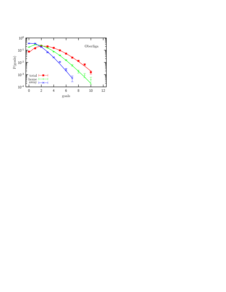
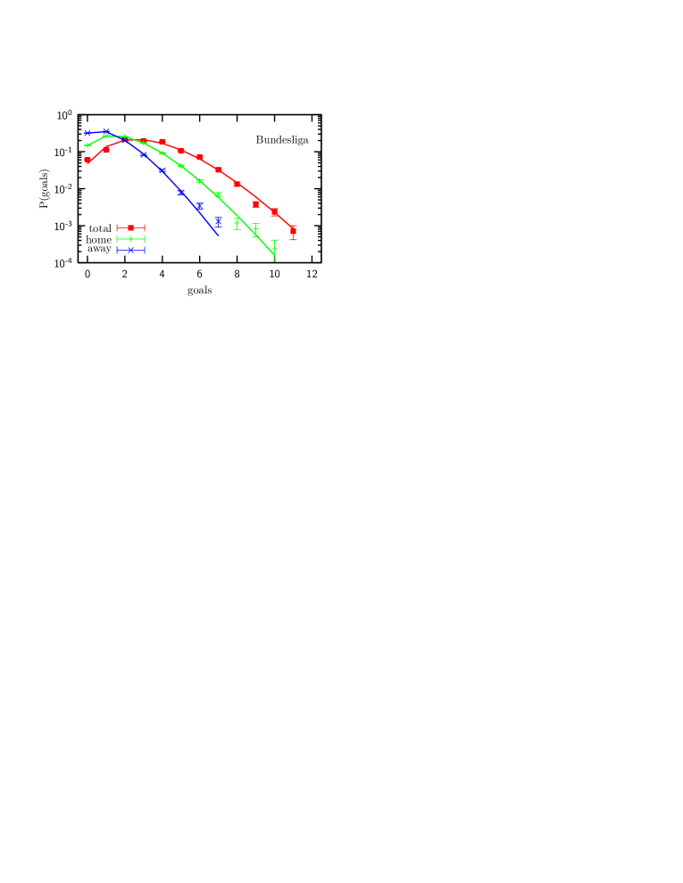
Figure 1: Probability density of goals scored by home teams, away teams, and of the total number of goals scored in the match. Left: “Oberliga” of the GDR between 1949 and 1990. Right: “Bundesliga” of the FRG in the seasons of 1963/64 – 1990/91. The lines for “home” and “away” show fits of the negative binomial distribution (4) to the data; the line for “total” denotes the resulting distribution of the sum, Eq. (5).

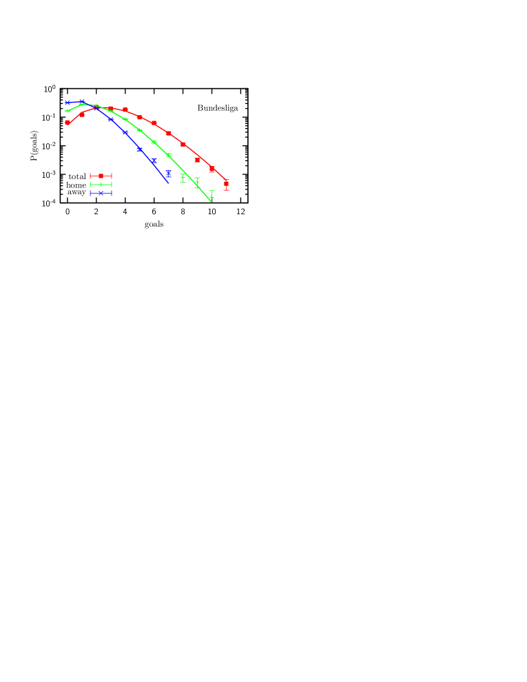
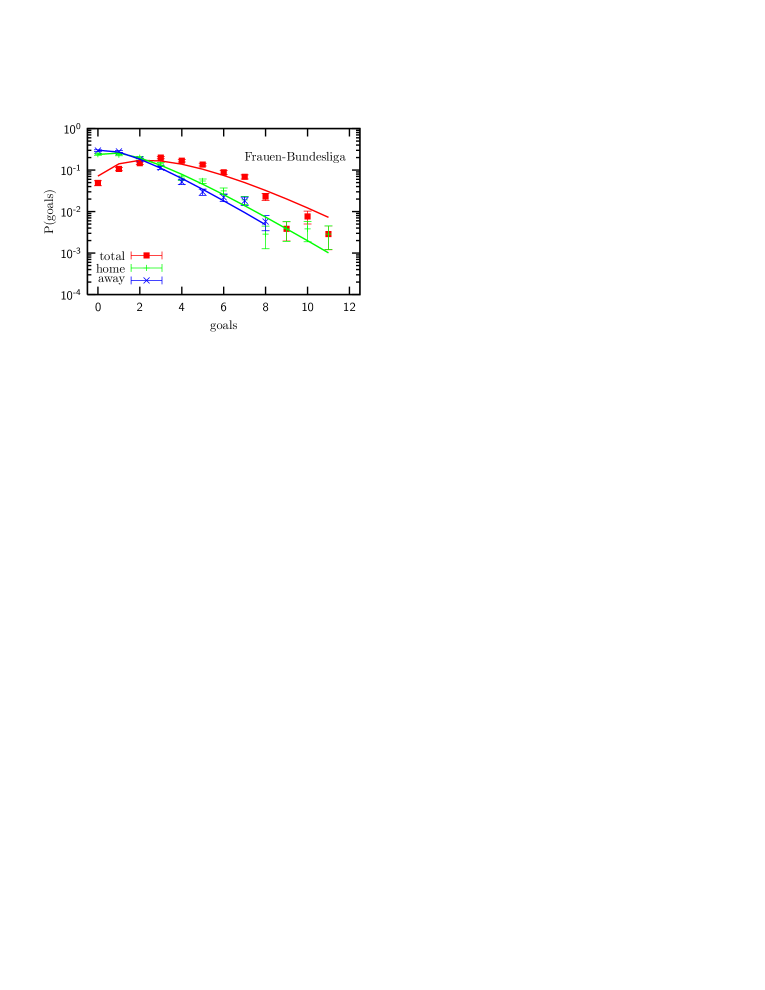
Figure 2: Probability density of goals scored in the German premier league “Bundesliga” for all seasons (left) and in the women’s “Frauen-Bundesliga” (right).

We first considered fits of the PDFs of the phenomenological descriptions considered previously, namely the Poissonian form (1), the negative binomial distribution (4) and the distributions (10) of extreme value statistics. The parameters of fits of these types to the data are summarized in Table 1 comparing the East German “Oberliga” to the West German “Bundesliga” (1963/64 – 1990/91, $\approx 8400$ matches) during the time of the German division, and in Table 2 comparing the data for all games of the German men’s premier league “Bundesliga” to the German women’s premier league “Frauen-Bundesliga”. Not to our surprise, and in accordance with previous findings reep:71 ; green , the simple Poissonian ansatz (1) is not found to be an adequate description for any of the data sets. Deviations occur here mainly in the tails with large numbers of goals which in general are found to be fatter than can be accommodated by a Poissonian model, whereas the distribution peaks are reasonably well represented. On the contrary, the negative binomial form (4) models all of the considered data well as is illustrated with fits of the corresponding form to our data in Fig. 1 comparing “Oberliga” and “Bundesliga” and in Fig. 2 presenting “Bundesliga” and “Frauen-Bundesliga”. Comparing the leagues, we find that the parameters $r$ of the NBD fits for the “Bundesliga” are about twice as large as for the “Oberliga”, whereas the parameters $p$ are smaller for the “Bundesliga”, cf. the data in Table 1. Recalling that the form (4) is in fact the continuum limit of the feedback model “A” discussed above, these differences translate into larger values of $\kappa$ and smaller values of $p_{0}$ for the “Oberliga” results. That is to say, scoring a goal in a match of the East German premier league was a more encouraging event than scoring a goal in a match of the West German league. Alternatively, this observation might be interpreted as a stronger tendency of the perhaps more professionalized teams of the West German league to switch to a strongly defensive mode of play in case of a lead. Consequently, the tails of the distributions are slightly fatter for the “Oberliga” than for the “Bundesliga”. Comparing the results for the “Frauen-Bundesliga” to those for the “Bundesliga”, even more pronounced tails are found for the former, resulting in very significantly larger values of the self-affirmation parameter $\kappa$ for the matches of the women’s league, see the fit parameters collected in Table 2 and the fits of the NBD type presented in Fig. 2.

Considering the fits of the GEV distributions (10) to the data for all three leagues, we find that extreme value statistics are in general a reasonably good description of the data. The shape parameter $\xi$ is always found to be small in modulus and negative in the majority of the cases, indicating a distribution of the Weibull type (which is in agreement with the findings of Ref. green ). On the other hand, fixing $\xi=0$ yields overall clearly larger values of $\chi^{2}$ per degree-of-freedom, indicating that the data are hardly compatible with a distribution of the Gumbel type. Comparing “Oberliga” and “Bundesliga”, we consistently find larger values of the parameter $\xi$ for the former, indicative of the comparatively fatter tails of these data discussed above, see the data in Table 1. The location parameter $\mu$, on the other hand, is larger for the West German league which features a larger average number of goals per match (which can be read off also more directly from the $\lambda$ parameter of the Poissonian fits), while the scale parameter $\sigma$ is similar for both leagues. Comparing to the results for the NBD, we do not find any cases where the GEV distributions would provide the best fit to the data, so clearly the leagues considered here are not of the type of the general “domestic” league data for which Greenhough et al. green found better matches with the GEV than for the NBD statistics. Similar conclusions hold true for the comparisons of “Bundesliga” and “Frauen-Bundesliga”, with the latter taking on the role of the “Oberliga”.

Assuming, for the time being, that the histograms of the final scores of the home and away teams are properly modeled by the fits presented in Tables 1 and 2, it is worthwhile as a consistency check to see whether the resulting estimates (2) and (5) of the PDFs for the Poisson and negative binomial distributions are consistent with the data for the sums and differences. Of course, such consistency can only be expected if the histograms of home and away scores are statistically independent, which assumption certainly is a strongly simplifying approximation. In Table 3 we summarize the mean squared deviations $\chi^{2}$ of the PDFs (2) resp. (5), evaluated with the parameters of the fits to the home and away scores of Tables 1 and 2, from the data for the sums and differences. While again clearly the Poissonian ansatz disqualifies as an acceptable model of the data, the NBD fits the data for the “Oberliga” and the “Frauen-Bundesliga” comparatively well, cf. the data in Table 3 and the “total” fits in Figs. 1 and 2. For the “Bundesliga”, however, significant deviations are observed. These deviations might go back to an effect of correlation between the home and away scores. To investigate this question we computed the empirical correlation coefficient,

$$R=\frac{\mathrm{Cov}(n_{\mathrm{h}},n_{\mathrm{a}})}{\sigma(n_{\mathrm{h}})\sigma(n_{\mathrm{a}})},$$ (11)

where $\sigma(n)$ denotes the square root of the variance of $n$ and $\mathrm{Cov}(n_{\mathrm{h}},n_{\mathrm{a}})$ the covariance of $n_{\mathrm{h}}$ and $n_{\mathrm{a}}$. We find $R=-0.015\pm 0.011$ for the “Oberliga” and $R=-0.031\pm 0.009$ for the “Bundesliga”, indicating stronger home-away score correlations for the “Bundesliga” fn2 .

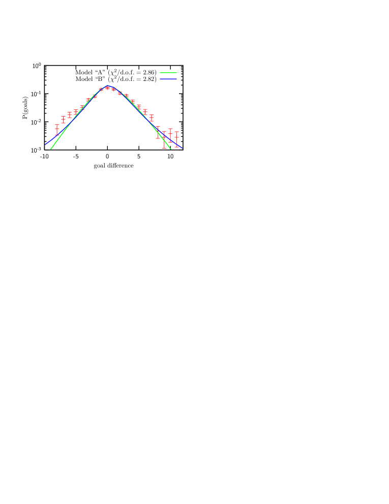
Figure 3: Goal differences in the German women’s premier league together with fits of models “A” and “B”.

In total, the best fits so far are clearly achieved by the NBD ansatz. Since this distribution is obtained only as the continuum limit of the microscopic model “A”, it is interesting to see how fits of the exact distribution (for $N=90$) resulting from the recurrence (8) for model “A”, but also fits of the multiplicatively modified binomial distribution of model “B” compare to the results found above. We perform fits to the exact distributions of both models by employing the simplex method num_rec to minimize the total $\chi^{2}$ of the data for the home and away scores. Alternatively, we also considered fitting additionally to the sums and differences in a simultaneous fit and found very similar results with an only slight improvement of the fit quality for the sums and differences at the expense of somewhat worse fits for the home and away scores. We summarize the fit results in Table 4. We also performed fits to the more elaborate model “C”, but found rather similar results to the simpler model “B” and hence do not present the results here. Comparing the results of model “A” to the fits of the limiting NBD, we find almost identical fit qualities for the final scores of both teams. However, the sums and differences of scores are considerably better described by model “A”, indicating that here the deviations from the continuum limit are still relevant. In Fig. 3, we present the differences of goals in the German women’s premier league together with the fits of models “A” and “B”. The multiplicative model “B”, where each goal motivates a team even more than the previous one, within the statistical errors yields fits of the same quality as model “A”, such that a distinct advantage cannot be attributed to either of them, cf. the data in Table 4.

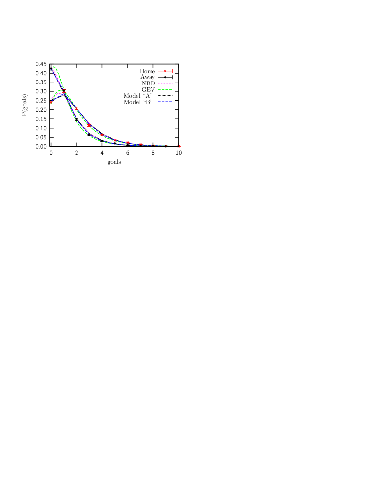
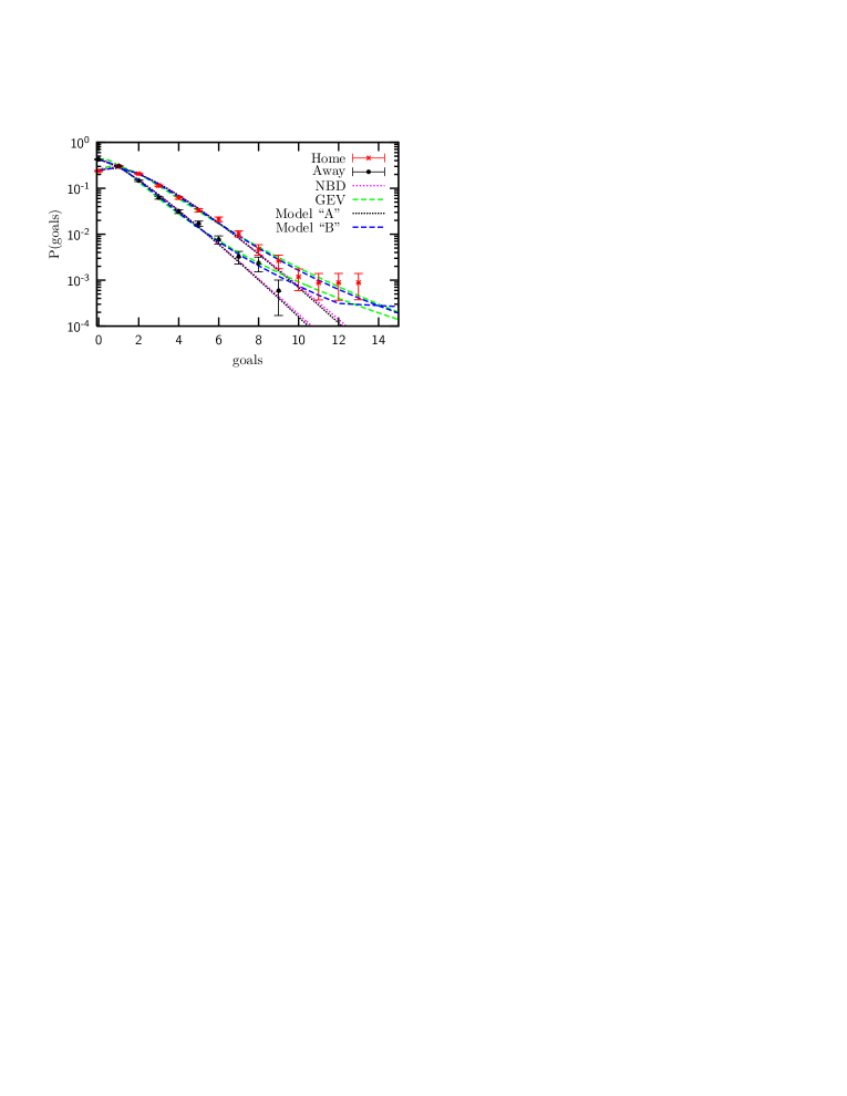
Figure 4: Probability density of goals scored by the home and away teams in the qualification stage of the “FIFA World Cup” series from 1930 to 2002.

Finally, to leave the realm of German football, we considered the score data of the “FIFA World Cup” series from 1930 to 2002, focusing on the results from the qualification stage ($\approx 3400$ matches) daten5  fn3 . The results of fits of the phenomenological distributions (1), (4) and (10) as well as the models “A” and “B” are collected in Table 5. Compared to the domestic league data discussed above, the results of the World Cup show distinctly heavier tails, cf. the presentation of the data in Fig. 4. Considering the fit results, this leads to good fits for the heavy-tailed distributions, and, in particular, in this case the GEV distribution provides a better fit than the negative binomial model, similar to what was found by Greenhough et al. green for some of their data. This difference to the German league data discussed above can be attributed to the possibly very large differences in skill between the opposing teams occurring since all countries are allowed to participate in the qualification round. A glance back to Table 2 reveals a remarkable similarity with the parameters of the “Frauen-Bundesliga” (e.g., in both cases the NBD parameters $p$ are comparatively large while $r$ is small, and the GEV parameters $\xi$ are positive), where a similar explanation appears quite plausible since the very good players are concentrated in two or three teams only. Turning to the fits of the models “A” and “B”, we again find model “A” to fit rather similar to its continuum approximation, the NBD. On the other hand, model “B” describes the data extremely well, for the away team even better than the GEV distributions (10). It is, of course, also possible and interesting to analyze the results from the final round. Similar to other cups such as the German “DFB-Pokal” we also considered, the rules are slightly different here, since no game can end in a draw, leading to special correlation effects in particular in the histograms of the goal differences. These problems will be investigated in a forthcoming publication.

IV Summary

We have considered German domestic and international football score data with respect to certain phenomenological probability distributions as well as microscopically motivated models. The Poisson distribution resulting from the assumption of independent scoring probabilities for the opposing teams does not provide a satisfactory fit to any of our data. Many data sets are rather well described by the negative binomial distribution considered before reep:71 , however, some cases have heavier tails than can be accommodated by this distribution and, instead, rather follow a distribution from extreme value statistics.

We have shown that football score data can be understood from a certain class of modified binomial models with a built-in effect of self-affirmation of the teams upon scoring a goal. The negative binomial distribution fitting many of the data sets can in fact be understood as a limiting distribution of our model “A” with an additive update rule of the scoring probability. It is found, however, that the exact distribution of model “A” provides in general rather better fits to the data than the limiting NBD, in particular concerning the sums and differences of goals scored. However, it does not provide very good fits in cases with heavier tails such as the qualification round of the “FIFA World Cup” series. The variant model “B”, on the other hand, where a multiplicative update rule ensures that each goal motivates the team even more than the previous one, fits these world-cup data as well as the data from the German domestic leagues extremely well. Thus, the contradicting evidence for better fits of some football score data with negative binomial and other data with GEV distributions is reconciled with the use of a plausible microscopic model covering both cases. We also analyzed results from further leagues, such as the Austrian, Belgian, British, Bulgarian, Czechoslovak, Dutch, French, Hungarian, Italian, Portuguese, Romanian, Russian, Scottish and Spanish premier leagues, and arrived at similar conclusions.

Comparing the score data between the separate German premier leagues during the cold war times, we find heavier tails for the East German league. In terms of our microscopic models, this corresponds to a stronger component of self-affirmation as compared to the West German league. Similarly, the German women’s premier league “Frauen-Bundesliga” shows a much stronger feedback effect than the men’s premier league, with at first sight surprisingly many parallels to the “FIFA World Cup” series. In general, we find less professionalized leagues to feature stronger components of positive feedback upon scoring a goal, perhaps indicating a still stronger infection with the football fever there …

It is obvious that the presented models with a single parameter of self-affirmation are a gross over-simplification of the complex psycho-social phenomena on a football pitch. It is all the more surprising then, how rather well they model the considered score distributions fn4 . Naturally, however, a plethora of opportunities for improvement of the description and further studies opens up. For instance, considering averages over whole leagues or cups, we have not taken into account the differences in skill between the teams. Likewise, if time-resolved scoring data were made available, a closer investigation of the intra-team and inter-team motivation and demotivation effects would provide an intriguing future enterprise to undertake.

Appendix A Probabilistics of correlated Bernoulli trials

Consider a series of $N$ Bernoulli random variables $U_{i}$, $i=1,\ldots,N$, with probabilities $1-p_{i}$ and $p_{i}$ for the outcomes “0” (“failure”) and “1” (“success”), respectively. We are interested in the distribution $P_{N}(\sum_{i=1}^{N}U_{i}=n)$ of the number of successes in $N$ trials. For the limiting case of equal and constant probabilities $p_{i}=p$, $i=1,\ldots,N$, the $U_{i}$ are i.i.d. random variables and $P_{N}$ is given by the binomial distribution

$$P_{N}(\sum_{i=1}^{N}U_{i}=n)={N\choose n}p^{n}\,(1-p)^{N-n},$$ (12)

which is a properly normalized (discrete) probability distribution function according to the binomial theorem. This can be generalized for arbitrary independent choices of probabilities $p_{i}$.

We discuss a more general case where, instead, the probabilities $p_{i}$ themselves depend on the number of previous successes, $p_{i}=p(\sum_{k=1}^{i-1}U_{i})$. Due to the introduced correlations, one should then consider the joint probability distribution of the $U_{i}$,

$$P(U_{1},\ldots,U_{N})=\prod_{i=1}^{N}\left\{p(\sum_{k=1}^{i-1}U_{k})\delta_{U_{i},1}+[1-p(\sum_{k=1}^{i-1}U_{k})]\delta_{U_{i},0}\right\},$$ (13)

from which the desired distribution of successes follows as the marginal $P_{N}(n)=\sum_{\{U_{i}\}}P(U_{1},\ldots,U_{N})\delta_{\sum U_{i},n}$. Instead of formally proceeding from (13) it is more convenient, however, to observe that the distances $D_{j}$ between subsequent successes are independent geometrically distributed random variables with probabilities $1-p(n)$, i.e. $P(D_{j}=d_{j})=p(j)[1-p(j)]^{d_{j}-1}$, $j=0,\ldots,n$, and the desired marginal distribution becomes

$$P_{N}(n) = \sum_{d_{0}=1}^{N-n}\cdots\sum_{d_{n}=1}^{N-n}\,[1-p(0)]^{d_{0}-1}p(0)\cdots p(n-1)[1-p(n)]^{d_{n}-1}\delta_{\sum_{j}d_{j},N}$$ (14)

$$= \prod_{j=0}^{n-1}p(j)\sum_{d_{0}=1}^{N-n}\cdots\sum_{d_{n}=1}^{N-n}\,\prod_{j=0}^{n}[1-p(j)]^{d_{j}-1}\,\delta_{\sum_{j}d_{j},N}.$$

Manipulating this form it is straightforward to prove a Pascal type recurrence relation for the probabilities $P_{N}(n)$,

$$P_{N}(n)=[1-p(n)]P_{N-1}(n)+p(n-1)P_{N-1}(n-1),$$ (15)

which together with the initial condition $P_{0}(0)=1$ and noting that $P_{N}(n)=0$ for $n>N$ allows to construct the distribution with an O($N^{2}$) computational effort compared to the formal O($2^{N}$) effort implied by Eq. (13). Multiplying (15) by $u^{n}$ and summing over all $n$, one arrives at

$$G_{N}(u)-G_{N-1}(u)=(u-1)H_{N-1}(u),$$ (16)

where

$$G_{N}(u)=\sum_{n=0}^{\infty}P_{N}(n)u^{n},\;\;\;H_{N}(u)=\sum_{n=0}^{\infty}p(n)P_{N}(n)u^{n},$$ (17)

such that $G_{N}(u)$ is the generating function of $P_{N}(n)$. The continuum limit $N\mapsto t$ is thus described by the differential equation

$$\frac{\partial G(u,t)}{\partial t}=(u-1)H(u,t).$$ (18)

The additive, correlated binomial model discussed in the main text modifies $p\mapsto p+\kappa$ on each success, unless $p+\kappa>1$ in which case $p\mapsto 1$. Restricting ourselves to the range of parameters where $p<1$, we have $p(n)=p_{0}+\kappa n$, $H_{N}(u)=p_{0}G_{N}(u)+\kappa u\frac{\partial}{\partial u}G_{N}(u)$ and Eq. (18) becomes

$$\frac{\partial G(u,t)}{\partial t}=(u-1)[p_{0}G(u,t)+\kappa u\frac{\partial}{\partial u}G(u,t)],$$ (19)

which is readily checked to be solved by

$$G(u,t)=[\mathrm{e}^{\kappa t}-u(\mathrm{e}^{\kappa t}-1)]^{-p_{0}/\kappa}.$$ (20)

Hence, $P(n)$ has a negative binomial distribution arbous:51 ; fisz ,

$$P_{t}(n)=\mathrm{e}^{-p_{0}t}\frac{\Gamma(p_{0}/\kappa+n)}{n!\,\Gamma(p_{0}/\kappa)}{\left(1-\mathrm{e}^{-\kappa t}\right)}^{n}={r+n-1\choose n}p^{n}(1-p)^{r},$$ (21)

where $r=p_{0}/\kappa$ and $p=1-\mathrm{e}^{-\kappa t}$. For $N\kappa=\mathrm{const}<1$, this continuum approximation is appropriate in the same limit where the Poissonian distribution is a valid approximation for the binomial distribution (12), i.e., for $N\gg 1$ with $Np_{o}=\mathrm{const}$.

For the multiplicative, correlated binomial model, after each success the probability is modified as $p\mapsto\kappa p$ (unless $\kappa p>1$, in which case $p\mapsto 1$), such that $p(j)=p_{0}\kappa^{j}$ for the range of parameters where $p(n)<1$. In this case, the differential equation (18) becomes

$$\frac{\partial G(u,t)}{\partial t}=(u-1)p_{0}G(\kappa u,t).$$ (22)

Note that due to the different first arguments of $G$, this is not an ordinary differential equation. We currently do not see how the solution could be expressed in terms of elementary or special functions in this case. Still, the distribution $P_{N}(n)$ can be easily computed from the recurrence (15) fn5 .

Finally, for the case of two coupled, correlated binomial distributions with probabilities $p_{A}$ for “success A”, $p_{B}$ for “success B” and $(1-p_{A}-p_{B})$ for “failure”, similar considerations lead to a recurrence relation

$$P_{N}(n_{A},n_{B}) = [1-p_{A}(n_{A},n_{B})-p_{B}(n_{A},n_{B})]P_{N-1}(n_{A},n_{B})+$$ (23)

$$p_{A}(n_{A}-1,n_{B})P_{N-1}(n_{A}-1,n_{B})+$$

$$p_{B}(n_{A},n_{B}-1)P_{N-1}(n_{A},n_{B}-1),$$

from which the distributions $P_{N}(n_{A},n_{B})$ for the model variants “A”, “B” and “C” can be easily computed in O($N^{3}$) time.

Table 1: Fits of the phenomenological distributions (1), (4) and (10) to the data for the East German “Oberliga” between 1949/50 and 1990/91 and for the West German “Bundesliga” for the seasons of 1963/64 – 1990/91.

		Oberliga		Bundesliga
		Home	Away	Home	Away
Poisson	$\lambda$	$1.85\pm 0.02$	$1.05\pm 0.01$	$2.01\pm 0.02$	$1.17\pm 0.01$
	$\chi^{2}/{\rm d.o.f.}$	$12.5$	$12.8$	$6.53$	$7.31$
NBD	$p$	$0.17\pm 0.01$	$0.14\pm 0.01$	$0.11\pm 0.01$	$0.10\pm 0.01$
	$r$	$9.06\pm 0.88$	$6.90\pm 0.84$	$15.9\pm 2.10$	$11.3\pm 1.84$
	$p_{0}$	$0.0191$	$0.0112$	$0.0213$	$0.0126$
	$\kappa$	$0.0021$	$0.0016$	$0.0013$	$0.0011$
	$\chi^{2}/{\rm d.o.f.}$	$0.99$	$4.09$	$0.68$	$2.29$
GEV	$\xi$	$-0.05\pm 0.01$	$0.02\pm 0.01$	$-0.09\pm 0.01$	$-0.01\pm 0.01$
	$\mu$	$1.12\pm 0.02$	$0.49\pm 0.02$	$1.28\pm 0.02$	$0.58\pm 0.02$
	$\sigma$	$1.30\pm 0.02$	$0.90\pm 0.02$	$1.36\pm 0.02$	$0.96\pm 0.02$
	$\chi^{2}/{\rm d.o.f.}$	$1.93$	$5.04$	$1.83$	$4.74$
Gumbel	$\mu$	$1.12\pm 0.02$	$0.48\pm 0.02$	$1.28\pm 0.02$	$0.59\pm 0.01$
	$\sigma$	$1.25\pm 0.01$	$0.92\pm 0.01$	$1.25\pm 0.01$	$0.95\pm 0.01$
	$\chi^{2}/{\rm d.o.f.}$	$4.13$	$4.65$	$12.9$	$4.06$

Table 2: Fits of the phenomenological distributions (1), (4) and (10) to the data for the German men’s premier league “Bundesliga” between 1963/64 and 2004/05 and for the German women’s premier league “Frauen-Bundesliga” for the seasons of 1997/98 – 2004/05.

		Bundesliga		Frauen-Bundesliga
		Home	Away	Home	Away
Poisson	$\lambda$	$1.91\pm 0.01$	$1.16\pm 0.01$	$1.78\pm 0.04$	$1.36\pm 0.04$
	$\chi^{2}/{\rm d.o.f.}$	$9.21$	$9.13$	$14.6$	$14.4$
NBD	$p$	$0.11\pm 0.01$	$0.09\pm 0.01$	$0.45\pm 0.03$	$0.46\pm 0.03$
	$r$	$16.24\pm 1.82$	$12.08\pm 1.69$	$2.38\pm 0.24$	$1.97\pm 0.22$
	$p_{0}$	$0.0202$	$0.0125$	$0.0160$	$0.0133$
	$\kappa$	$0.0012$	$0.0010$	$0.0067$	$0.0068$
	$\chi^{2}/{\rm d.o.f.}$	$1.08$	$2.22$	$2.32$	$1.37$
GEV	$\xi$	$-0.10\pm 0.01$	$-0.02\pm 0.01$	$0.04\pm 0.04$	$0.25\pm 0.07$
	$\mu$	$1.17\pm 0.02$	$0.57\pm 0.01$	$0.83\pm 0.08$	$0.77\pm 0.07$
	$\sigma$	$1.33\pm 0.01$	$0.96\pm 0.01$	$1.49\pm 0.06$	$1.18\pm 0.05$
	$\chi^{2}/{\rm d.o.f.}$	$3.43$	$7.95$	$3.40$	$1.55$
Gumbel	$\mu$	$1.18\pm 0.01$	$0.58\pm 0.01$	$0.81\pm 0.08$	$0.58\pm 0.07$
	$\sigma$	$1.21\pm 0.01$	$0.94\pm 0.01$	$1.53\pm 0.05$	$1.31\pm 0.05$
	$\chi^{2}/{\rm d.o.f.}$	$24.5$	$7.26$	$3.17$	$4.09$

Table 3: Matching of the sums and differences of goals. Fits were performed to the home and away score distributions only and mean-squared deviations were computed for the distributions of sums and differences from Eqs. (2) and (5) with the thus found parameters $\lambda_{h}$ and $\lambda_{a}$ resp. $p_{\rm h}$, $r_{\rm h}$, $p_{\rm a}$ and $r_{\rm a}$.

		Bundesliga 04/05	Bundesliga 90/91	Oberliga	Women
Poisson	$\lambda_{h}$	$1.91\pm 0.01$	$2.01\pm 0.02$	$1.85\pm 0.02$	$1.78\pm 0.04$
	$\lambda_{a}$	$1.16\pm 0.01$	$1.17\pm 0.01$	$1.05\pm 0.01$	$1.36\pm 0.04$
Home	$\chi^{2}_{\rm h}/{\rm d.o.f.}$	$9.21$	$6.53$	$12.5$	$14.6$
Away	$\chi^{2}_{\rm a}/{\rm d.o.f.}$	$9.13$	$7.31$	$12.8$	$14.4$
Total	$\chi^{2}_{\Sigma}/{\rm d.o.f.}$	$10.7$	$15.9$	$16.3$	$10.4$
Difference	$\chi^{2}_{\Delta}/{\rm d.o.f.}$	$67.6$	$578$	$474$	$20.2$
NBD	$p_{h}$	$0.11\pm 0.01$	$0.11\pm 0.01$	$0.17\pm 0.01$	$0.45\pm 0.03$
	$r_{h}$	$16.24\pm 1.82$	$15.9\pm 2.10$	$9.06\pm 0.82$	$2.38\pm 0.24$
	$p_{a}$	$0.09\pm 0.01$	$0.10\pm 0.01$	$0.14\pm 0.01$	$0.46\pm 0.03$
	$r_{a}$	$12.08\pm 1.69$	$11.3\pm 1.84$	$6.90\pm 0.84$	$1.97\pm 0.22$
Home	$\chi^{2}_{\rm h}/{\rm d.o.f.}$	$1.08$	$0.68$	$0.99$	$2.32$
Away	$\chi^{2}_{\rm a}/{\rm d.o.f.}$	$2.22$	$2.29$	$4.09$	$1.37$
Total	$\chi^{2}_{\Sigma}/{\rm d.o.f.}$	$25.1$	$17.3$	$8.31$	$18.9$
Difference	$\chi^{2}_{\Delta}/{\rm d.o.f.}$	$23.9$	$18.0$	$7.16$	$3.55$

Table 4: Fit results for models “A” and “B”. Fits were performed to the score distributions of the home and away teams only and the resulting model estimates for the sums and differences of goals compared to the data.

		Bundesliga 04/05	Bundesliga 90/91	Oberliga	Women
Model “A”	$p_{0,\rm h}$	$0.0199\pm 0.0002$	$0.0210\pm 0.0002$	$0.0188\pm 0.0002$	$0.0159\pm 0.0005$
	$\kappa_{\rm h}$	$0.0015\pm 0.0001$	$0.0016\pm 0.0002$	$0.0024\pm 0.0002$	$0.0070\pm 0.0005$
	$p_{0,\rm a}$	$0.0125\pm 0.0002$	$0.0125\pm 0.0001$	$0.0112\pm 0.0001$	$0.0132\pm 0.0004$
	$\kappa_{\rm a}$	$0.0012\pm 0.0001$	$0.0013\pm 0.0002$	$0.0018\pm 0.0002$	$0.0071\pm 0.0007$
Home	$\chi^{2}_{\rm h}/{\rm d.o.f.}$	$1.01$	$0.68$	$1.07$	$2.28$
Away	$\chi^{2}_{\rm a}/{\rm d.o.f.}$	$2.31$	$2.37$	$4.23$	$1.44$
Total	$\chi^{2}_{\Sigma}/{\rm d.o.f.}$	$16.6$	$11.5$	$5.33$	$12.4$
Difference	$\chi^{2}_{\Delta}/{\rm d.o.f.}$	$18.6$	$14.0$	$5.63$	$2.86$
Model “B”	$p_{0,\rm h}$	$0.0200\pm 0.0002$	$0.0211\pm 0.0002$	$0.0189\pm 0.0002$	$0.0166\pm 0.0005$
	$\kappa_{\rm h}$	$1.0679\pm 0.0060$	$1.0695\pm 0.0072$	$1.1115\pm 0.0083$	$1.3146\pm 0.0303$
	$p_{0,\rm a}$	$0.0125\pm 0.0001$	$0.0125\pm 0.0002$	$0.0112\pm 0.0001$	$0.0138\pm 0.0004$
	$\kappa_{\rm a}$	$1.0932\pm 0.0106$	$1.1015\pm 0.0124$	$1.1526\pm 0.0149$	$1.4115\pm 0.0543$
Home	$\chi^{2}_{\rm h}/{\rm d.o.f.}$	$1.25$	$0.71$	$0.75$	$3.24$
Away	$\chi^{2}_{\rm a}/{\rm d.o.f.}$	$1.96$	$2.02$	$3.35$	$0.95$
Total	$\chi^{2}_{\Sigma}/{\rm d.o.f.}$	$16.9$	$11.8$	$5.40$	$13.5$
Difference	$\chi^{2}_{\Delta}/{\rm d.o.f.}$	$18.4$	$13.8$	$5.26$	$2.82$

Table 5: Fit results for the qualification phase of the “FIFA World Cup” series from 1930 to 2002.

		Home	Away
Poisson	$\lambda$	$1.53\pm 0.02$	$0.89\pm 0.01$
	$\chi^{2}/{\rm d.o.f.}$	$18.6$	$25.0$
NBD	$p$	$0.37\pm 0.02$	$0.38\pm 0.02$
	$r$	$3.04\pm 0.21$	$1.76\pm 0.12$
	$p_{0}$	$0.0154$	$0.0094$
	$\kappa$	$0.0051$	$0.0053$
	$\chi^{2}/{\rm d.o.f.}$	$2.67$	$2.02$
GEV	$\xi$	$0.11\pm 0.02$	$0.19\pm 0.02$
	$\mu$	$0.86\pm 0.03$	$0.36\pm 0.03$
	$\sigma$	$1.21\pm 0.03$	$0.86\pm 0.02$
	$\chi^{2}/{\rm d.o.f.}$	$0.85$	$1.89$
Gumbel	$\mu$	$0.80\pm 0.03$	$0.25\pm 0.03$
	$\sigma$	$1.31\pm 0.02$	$0.94\pm 0.02$
	$\chi^{2}/{\rm d.o.f.}$	$3.29$	$12.9$
Model “A”	$p_{0}$	$0.0152\pm 0.0003$	$0.0093\pm 0.0002$
	$\kappa$	$0.0053\pm 0.0003$	$0.0055\pm 0.0003$
	$\chi^{2}/{\rm d.o.f.}$	$2.88$	$2.19$
Model “B”	$p_{0}$	$0.0155\pm 0.0002$	$0.0095\pm 0.0002$
	$\kappa$	$1.2780\pm 0.0130$	$1.4775\pm 0.0343$
	$\chi^{2}/{\rm d.o.f.}$	$0.92$	$0.80$

References

- (1) D. Stauffer, Physica A336 (2004) 1.
- (2) M. J. Moroney, Facts from Figures, 3rd edition (Penguin, London, 1956).
- (3) C. Reep, R. Pollard, and B. Benjamin, J. Roy. Stat. Soc. A134 (1971) 623.
- (4) R. Pollard, J. Am. Stat. Assoc. 68 (1973) 351.
- (5) S. R. Clarke and J. M. Norman, The Statistician 44 (1995) 509.
- (6) D. Dyte and S. R. Clarke, J. Op. Res. Soc. 51 (2000) 993.
- (7) L. C. Malacarne and R. Mendes, Physica A286 (2000) 391.
- (8) J. Greenhough, P. C. Birch, S. C. Chapman, and G. Rowlands, Physica A316 (2002) 615.
- (9) A. G. Arbous and J. E. Kerrich, Biometrics 7 (1951) 340.
- (10) S. Kotz and S. Nadarajah, Extreme Value Distributions: Theory and Applications (World Scientific, Singapore, 2000)
- (11) S. T. Bramwell, P. C. W. Holdsworth, and J.-F. Pinton, Nature 396 (1998) 552.
- (12) S. T. Bramwell, K. Christensen, J.-Y. Fortin, P. C. W. Holdsworth, H. J. Jensen, S. Lise, J. M. López, M. Nicodemi, J.-F. Pinton, and M. Sellitto, Phys. Rev. Lett. 84 (2000) 3744.
- (13) J.-P. Bouchaud and M. Mézard, J. Phys. A30 (1997) 7997.
- (14) B. A. Berg, A. Billoire, and W. Janke, Phys. Rev. E65 (2002) 045102(R).
- (15) P. Dayal, S. Trebst, S. Wessel, D. Würtz, M. Troyer, S. Sabhapandit, and S. N. Coppersmith, Phys. Rev. Lett. 92 (2004) 097201.
- (16) E. Bittner and W. Janke, Europhys. Lett. 74 (2006) 195.
- (17) A. Noullez and J.-F. Pinton, Eur. Phys. J. B28 (2002) 231.
- (18) P. A. Varotsos, N. V. Sarlis, H. K. Tanaka, and E. S. Skordas, Phys. Rev. E72 (2005) 041103.
- (19) K. Dahlstedt and H. J. Jensen, J. Phys. A34 (2001) 11193.
- (20) E. Bertin, Phys. Rev. Lett. 95 (2005) 170601.
- (21) E. Bertin and M. Clusel, Generalised extreme value statistics and sum of correlated variables, Preprint cond-mat/0601189.
- (22) M. Abramowitz and I. A. Stegun, Handbook of Mathematical Functions (Dover Publications, New York, 1970).
- (23) M. Fisz, Wahrscheinlichkeitsrechnung und Mathematische Statistik (VEB Deutscher Verlag der Wissenschaften, Berlin, 1989).
- (24) W. Feller, An Introduction to Probability Theory and its Applications, vol. 1, 3rd edition (Wiley, New York, 1968).
- (25) Z. Drezner and N. Farnum, Comm. Stat. Theor. Meth. 22 (1993) 3051.
- (26) Z. Drezner, Comm. Stat. Theor. Meth. 35 (2006) 209.
- (27) http://www.fussballdaten.de
- (28) http://www.fussballportal.de
- (29) http://www.nordostfussball.de
- (30) http://www.sportergebnise.de
- (31) To ensure reliable error estimates, in the fits presented below we ignored histogram bins consisting of single or isolated entries, i.e., outliers.
- (32) B. Efron, SIAM Review 21 (1979) 460.
- (33) The available statistics for the “Frauen-Bundesliga” is too small to allow a meaningful estimation of .
- (34) W. H. Press, S. A. Teukolsky, W. T. Vetterling, and B. P. Flannery, Numerical Recipes in C — The Art of Scientific Computing, 2nd edition (CUP, Cambridge, 1992).
- (35) http://www.rdasilva.demon.co.uk/football.html
- (36) We disregarded all games played in tournaments on neutral grounds.
- (37) Also, on this level of abstraction it cannot be excluded that we are, in fact, observing an effect of spurious contagion as occurring for the negative bimodal distribution, which results as limiting distribution from non-contagious situations (as compound Poisson distribution) and contagious models (our model “A”). See also Ref. feller .
-
(38)
Alternatively, is the coefficient of the term of the power series expansion of
in powers of , where . We thank O. Penrose for pointing this out to us. Using a saddle-point calculation for the Cauchy integral representation of , a very accurate closed-form approximation can be derived, which will be reported elsewhere.