An outlook on correlations in stock prices

Abstract

We present an outlook of the studies on correlations in the price time-series of stocks, discussing the construction and applications of ”asset tree”. The topic discussed here should illustrate how the complex economic system (financial market) enrichens the list of existing dynamical systems that physicists have been studying for long.

“If stock market experts were so expert, they would be buying stock, not selling advice.”
– Norman Augustine, US aircraft businessman (1935 - )

I Introduction

The word “correlation” is defined as “a relation existing between phenomena or things or between mathematical or statistical variables which tend to vary, be associated, or occur together in a way not expected on the basis of chance alone” (see http://www.m-w.com/dictionary/correlations). As soon as we talk about “chance”, the words “probability”,“random”, etc come to our mind. So, when we talk about correlations in stock prices, what we are really interested in are the nature of the time series of stock prices, the relation of stock prices with other variables like stock transaction volumes, the statistical distributions and laws which govern the price time series, in particular whether the time series is random or not. The first formal efforts in this direction were those of Louis Bachelier, more than a century ago Bachelier . Eversince, financial time series analysis is of prevalent interest to theoreticians for making inferences and predictions though it is primarily an empirical discipline. The uncertainty in the financial time series and its theory makes it specially interesting to statistical physicists, besides financial economists tsay ; santha . One of the most debatable issues in financial economics is whether the market is “efficient” or not. The “efficient” asset market is one in which the information contained in past prices is instantly, fully and continually reflected in the asset’s current price. As a consequence, the more efficient the market is, the more random is the sequence of price changes generated by the market. Hence, the most efficient market is one in which the price changes are completely random and unpredictable. This leads to another relevant or pertinent question of financial econometrics: whether asset prices are predictable. Two simplest models of probability theory and financial econometrics that deal with predicting future price changes, the random walk theory and Martingale theory, assume that the future price changes are functions of only the past price changes. Now, in Economics the “logarithmic returns” is calculated using the formula

$$r(t)=\ln P(t)-\ln P(t-1),$$ (1)

where $P(t)$ is the price (index) at time step $t$. A main characteristic of the random walk and Martingale models is that the returns are uncorrelated.

In the past, several hypotheses have been proposed to model financial time series and studies have been conducted to explain their most characteristic features. The study of long-time correlations in the financial time series is a very interesting and widely studied problem, especially since they give a deep insight about the underlying processes that generate the time series stanley . The complex nature of financial time series (see Fig. 1) has especially forced the physicists to add this system to their existing list of dynamical systems that they study. Here, we will not try to review all the studies, but instead give a brief outlook of the studies done by the author and his collaborators, and the motivated readers are kindly asked to refer the original papers for further details.

II Analysing Correlations in Stock Price time series

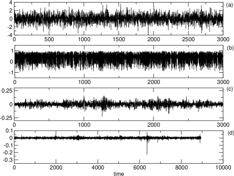
Figure 1: Comparison of several time series which are of interest to physicists and economists: (a) Random time series (3000 time steps) using random numbers from a Normal distribution with zero mean and unit standard deviation. (b) Multivariate spatio-temporal time series (3000 time steps) drawn from the class of diffusively coupled map lattices in one-dimension with sites $i=1,2...n^{\prime}$ of the form: $y_{t+1}^{i}=(1-\epsilon)f(y_{t}^{i})+\frac{\epsilon}{2}(f(y_{t}^{i+1})+f(y_{t}^{i-1}))$, where $f(y)=1-ay^{2}$ is the logistic map whose dynamics is controlled by the parameter $a$, and the parameter $\epsilon$ is a measure of coupling between nearest-neighbor lattice sites. We use parameters $a=1.97$, $\epsilon=0.4$ for the dynamics to be in the regime of spatio-temporal chaos. We choose $n=500$ and iterate, starting from random initial conditions, for $p=5\times 10^{7}$ time steps, after discarding $10^{5}$ transient iterates. Also, we choose periodic boundary conditions, $x(n+1)=x(1)$. (c) Multiplicative stochastic process GARCH(1,1) for a random variable $x_{t}$ with zero mean and variance $\sigma_{t}^{2}$, characterized by a Gaussian conditional probability distribution function $f_{t}(x)$: $\sigma_{t}^{2}=\alpha_{0}+\alpha_{1}x_{t-1}^{2}+\beta_{1}\sigma_{t-1}^{2}$, using parameters $\alpha_{0}=0.00023$, $\alpha_{1}=0.09$ and $\beta_{1}=0.01$ (3000 time steps). (d) Empirical Return time series of the S&P500 stock index (8938 time steps).

II.1 Financial Correlation matrix and constructing Asset Trees

In our studies, we used two different sets of financial data for different purposes. The first set from the Standard & Poor’s 500 index (S&P500) of the New York Stock Exchange (NYSE) from July 2, 1962 to December 31, 1997 containing 8939 daily closing values, which we have already plotted in Fig. 1(d). In the second set, we study the split-adjusted daily closure prices for a total of $N=477$ stocks traded at the New York Stock Exchange (NYSE) over the period of 20 years, from 02-Jan-1980 to 31-Dec-1999. This amounts a total of 5056 price quotes per stock, indexed by time variable $\tau=1,2,\ldots,5056$. For analysis and smoothing purposes, the data is divided time-wise into $M$ windows $t=1,\,2,...,\,M$ of width $T$, where $T$ corresponds to the number of daily returns included in the window. Several consecutive windows overlap with each other, the extent of which is dictated by the window step length parameter $\delta T$, which describes the displacement of the window and is also measured in trading days. The choice of window width is a trade-off between too noisy and too smoothed data for small and large window widths, respectively. The results presented in this paper were calculated from monthly stepped four-year windows, i.e. $\delta T=250/12\approx 21$ days and $T=1000$ days. We have explored a large scale of different values for both parameters, and the cited values were found optimal jpo . With these choices, the overall number of windows is $M=195$.

In order to investigate correlations between stocks we first denote the closure price of stock $i$ at time $\tau$ by $P_{i}(\tau)$ (Note that $\tau$ refers to a date, not a time window). We focus our attention to the logarithmic return of stock $i$, given by $r_{i}(\tau)=\ln P_{i}(\tau)-\ln P_{i}(\tau-1)$ which for a sequence of consecutive trading days, i.e. those encompassing the given window $t$, form the return vector $\bm{r}_{i}^{t}$. In order to characterize the synchronous time evolution of assets, we use the equal time correlation coefficients between assets $i$ and $j$ defined as

$$\rho_{ij}^{t}=\frac{\langle\bm{r}_{i}^{t}\bm{r}_{j}^{t}\rangle-\langle\bm{r}_{i}^{t}\rangle\langle\bm{r}_{j}^{t}\rangle}{\sqrt{[\langle{\bm{r}_{i}^{t}}^{2}\rangle-\langle\bm{r}_{i}^{t}\rangle^{2}][\langle{\bm{r}_{j}^{t}}^{2}\rangle-\langle\bm{r}_{j}^{t}\rangle^{2}]}},$$ (2)

where $\left\langle...\right\rangle$ indicates a time average over the consecutive trading days included in the return vectors. These correlation coefficients fulfill the condition $-1\leq\rho_{ij}\leq 1$. If $\rho_{ij}=1$, the stock price changes are completely correlated; if $\rho_{ij}=0$, the stock price changes are uncorrelated and if $\rho_{ij}=-1$, then the stock price changes are completely anti-correlated jp . These correlation coefficients form an $N\times N$ correlation matrix $\mathbf{C}^{t}$, which serves as the basis for trees discussed in this paper.

We construct an asset tree according to the methodology by Mantegna Man1 . For the purpose of constructing asset trees, we define a distance between a pair of stocks. This distance is associated with the edge connecting the stocks and it is expected to reflect the level at which the stocks are correlated. We use a simple non-linear transformation $d^{t}_{ij}=\sqrt{2(1-\rho_{ij}^{t})}$ to obtain distances with the property $2\geq d_{ij}\geq 0$, forming an $N\times N$ symmetric distance matrix $\mathbf{D}^{t}$. So, if $d_{ij}=0$, the stock price changes are completely correlated; if $d_{ij}=2$, the stock price changes are completely anti-uncorrelated. The trees for different time windows are not independent of each other, but form a series through time. Consequently, this multitude of trees is interpreted as a sequence of evolutionary steps of a single dynamic asset tree. We also require an additional hypothesis about the topology of the metric space, the ultrametricity hypothesis. In practice, it leads to determining the minimum spanning tree (MST) of the distances, denoted $\mathbf{T}^{t}$. The spanning tree is a simply connected acyclic (no cycles) graph that connects all $N$ nodes (stocks) with $N-1$ edges such that the sum of all edge weights, $\sum_{d_{ij}^{t}\in\mathbf{T}^{t}}d_{ij}^{t}$, is minimum. We refer to the minimum spanning tree at time $t$ by the notation $\mathbf{T}^{t}=(V,E^{t})$, where $V$ is a set of vertices and $E^{t}$ is a corresponding set of unordered pairs of vertices, or edges. Since the spanning tree criterion requires all $N$ nodes to be always present, the set of vertices $V$ is time independent, which is why the time superscript has been dropped from notation. The set of edges $E^{t}$, however, does depend on time, as it is expected that edge lengths in the matrix $\mathbf{D}^{t}$ evolve over time, and thus different edges get selected in the tree at different times.

II.2 Market characterization

We plot the distribution of (i) distance elements $d^{t}_{ij}$ contained in the distance matrix $\mathbf{D}^{t}$ (Fig. 2), (ii) distance elements $d_{ij}$ contained in the asset (minimum spanning) tree $\mathbf{T}^{t}$ (Fig. 3). In both plots, but most prominently in Fig. 2, there appears to be a discontinuity in the distribution between roughly 1986 and 1990. The part that has been cut out, pushed to the left and made flatter, is a manifestation of Black Monday (October 19, 1987), and its length along the time axis is related to the choice of window width $T$ bali ; jp .

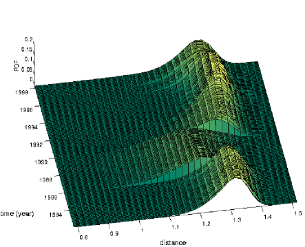
Figure 2: Distribution of all $N(N-1)/2$ distance elements $d_{ij}$ contained in the distance matrix $\mathbf{D}^{t}$ as a function of time.

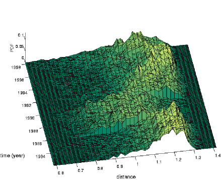
Figure 3: Distribution of the $(N-1)$ distance elements $d_{ij}$ contained in the asset (minimum spanning) tree $\mathbf{T}^{t}$ as a function of time.

Also, note that in the distribution of tree edges in Fig. 3 most edges included in the tree seem to come from the area to the right of the value 1.1 in Fig. 2, and the largest distance element is $d_{max}=1.3549$.

II.2.1 Tree occupation and central vertex

We focus on characterizing the spread of nodes on the tree, by introducing the quantity of mean occupation layer

$$l(t,v_{c})=\frac{1}{N}\sum_{i=1}^{N}\mathop{\mathrm{lev}}(v_{i}^{t}),$$ (3)

where $\mathop{\mathrm{lev}}(v_{i})$ denotes the level of vertex $v_{i}$. The levels, not to be confused with the distances $d_{ij}$ between nodes, are measured in natural numbers in relation to the central vertex $v_{c}$, whose level is taken to be zero. Here the mean occupation layer indicates the layer on which the mass of the tree, on average, is conceived to be located. The central vertex is considered to be the parent of all other nodes in the tree, and is also known as the root of the tree. It is used as the reference point in the tree, against which the locations of all other nodes are relative. Thus all other nodes in the tree are children of the central vertex. Although there is an arbitrariness in the choice of the central vertex, we propose that it is central, in the sense that any change in its price strongly affects the course of events in the market on the whole. We have proposed three alternative definitions for the central vertex in our studies, all yielding similar and, in most cases, identical outcomes. The idea here is to find the node that is most strongly connected to its nearest neighbors. For example, according to one definition, the central node is the one with the highest vertex degree, i.e. the number of edges which are incident with (neighbor of) the vertex. Also, one may have either (i) static (fixed at all times) or (ii) dynamic (updated at each time step) central vertex, but again the results do not seem to vary significantly. We can then study the variation of the topological properties and nature of the trees, with time. This type of visualization tool can sometimes provide deeper insight of the dynamical system.

II.2.2 Economic taxonomy

Mantegna’s idea of linking stocks in an ultrametric space was motivated a posteriori by the property of such a space to provide a meaningful economic taxonomy. In Man1 , Mantegna examined the meaningfulness of the taxonomy by comparing the grouping of stocks in the tree with a third party reference grouping of stocks by their industry etc. classifications. In this case, the reference was provided by Forbesforbes , which uses its own classification system, assigning each stock with a sector (higher level) and industry (lower level) category. In order to visualize the grouping of stocks, we constructed a sample asset tree for a smaller dataset (shown in Fig. 4)

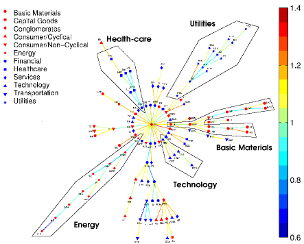
Figure 4: Snapshot of a dynamic asset tree connecting the examined 116 stocks of the S&P 500 index. The tree was produced using four-year window width and it is centered on January 1, 1998. Business sectors are indicated according to Forbes, http://www.forbes.com. In this tree, General Electric (GE) was used as the central vertex and eight layers can be identified.

short , which consists of 116 S&P 500 stocks, extending from the beginning of 1982 to the end of 2000, resulting in a total of 4787 price quotes per stock supp . The window width was set at $T=1000$, and the shown sample tree is located time-wise at $t=t^{*}$, corresponding to 1.1.1998. The stocks in this dataset fall into 12 sectors, which are Basic Materials, Capital Goods, Conglomerates, Consumer/Cyclical, Consumer/Non-Cyclical, Energy, Financial, Healthcare, Services, Technology, Transportation and Utilities. The sectors are indicated in the tree (see Fig. 4) with different markers, while the industry classifications are omitted for reasons of clarity. We use the term sector exclusively to refer to the given third party classification system of stocks. The term branch refers to a subset of the tree, to all the nodes that share the specified common parent. In addition to the parent, we need to have a reference point to indicate the generational direction (i.e. who is who’s parent) in order for a branch to be well defined. Without this reference there is absolutely no way to determine where one branch ends and the other begins. In our case, the reference is the central node. There are some branches in the tree, in which most of the stocks belong to just one sector, indicating that the branch is fairly homogeneous with respect to business sectors. This finding is in accordance with those of Mantegna Man1 , although there are branches that are fairly heterogeneous, such as the one extending directly downwards from the central vertex (see Fig. 4).

II.3 Portfolio analysis

Next, we apply the above discussed concepts and measures to the portfolio optimization problem, a basic problem of financial analysis. This is done in the hope that the asset tree could serve as another type of quantitative approach to and/or visualization aid of the highly inter-connected market, thus acting as a tool supporting the decision making process. We consider a general Markowitz portfolio $\mathbf{P}(t)$ with the asset weights $w_{1},\,w_{2},\ldots,\,w_{N}$. In the classic Markowitz portfolio optimization scheme, financial assets are characterized by their average risk and return, where the risk associated with an asset is measured by the standard deviation of returns. The Markowitz optimization is usually carried out by using historical data. The aim is to optimize the asset weights so that the overall portfolio risk is minimized for a given portfolio return $r_{\mathbf{P}}$. In the dynamic asset tree framework, however, the task is to determine how the assets are located with respect to the central vertex.

Let $r_{m}$ and $r_{M}$ denote the returns of the minimum and maximum return portfolios, respectively. The expected portfolio return varies between these two extremes, and can be expressed as $r_{\mathbf{P},\theta}=(1-\theta)r_{m}+\theta r_{M}$, where $\theta$ is a fraction between 0 and 1. Hence, when $\theta=0$, we have the minimum risk portfolio, and when $\theta=1$, we have the maximum return (maximum risk) portfolio. The higher the value of $\theta$, the higher the expected portfolio return $r_{\mathbf{P},\theta}$ and, consequently, the higher the risk the investor is willing to absorb. We define a single measure, the weighted portfolio layer as

$$l_{\mathbf{P}}(t,\theta)=\sum_{i\in\mathbf{P}(t,\theta)}w_{i}\mathop{\mathrm{lev}}(v_{i}^{t}),$$ (4)

where $\sum_{i=1}^{N}w_{i}=1$ and further, as a starting point, the constraint $w_{i}\geq 0$ for all $i$, which is equivalent to assuming that there is no short-selling. The purpose of this constraint is to prevent negative values for $l_{\mathbf{P}}(t)$, which would not have a meaningful interpretation in our framework of trees with central vertex. This restriction will shortly be discuss further.

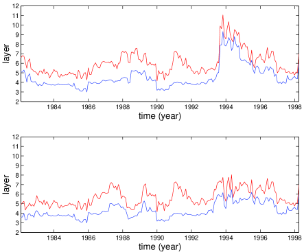
Figure 5: Plot of the weighted minimum risk portfolio layer $l_{\mathbf{P}}(t,\theta=0)$ with no short-selling and mean occupation layer $l(t,v_{c})$ against time. Top: static central vertex, bottom: dynamic central vertex according to the vertex degree criterion.

Fig. 5 shows the behavior of the mean occupation layer $l(t)$ and the weighted minimum risk portfolio layer $l_{\mathbf{P}}(t,\theta=0)$. We find that the portfolio layer is higher than the mean layer at all times. The difference between the layers depends on the window width, here set at $T=1000$, and the type of central vertex used. The upper plot in Fig. 5 is produced using the static central vertex (GE), and the difference in layers is found to be 1.47. The lower one is produced by using a dynamic central vertex, selected with the vertex degree criterion, in which case the difference of 1.39 is found. Here, we had assumed the no short-selling condition. However, it turns out that, in practice, the weighted portfolio layer never assumes negative values and the short-selling condition, in fact, is not necessary. Only minor differences are observed in the results between banning and allowing short-selling. Further, the difference in layers is also slightly larger for static than dynamic central vertex, although not by a significant amount.

As the stocks of the minimum risk portfolio are found on the outskirts of the tree, we expect larger trees (higher $L$) to have greater diversification potential, i.e., the scope of the stock market to eliminate specific risk of the minimum risk portfolio. In order to look at this, we calculated the mean-variance frontiers for the ensemble of 477 stocks using $T=1000$ as the window width. If we study the level of portfolio risk as a function of time, we find a similarity between the risk curve and the curves of the mean correlation coefficient $\bar{\rho}$ and normalized tree length $L$ jp . Earlier, when the smaller dataset of 116 stocks - consisting primarily important industry giants - was used, we found Pearson’s linear correlation between the risk and the mean correlation coefficient $\bar{\rho}(t)$ to be $0.82$, while that between the risk and the normalized tree length $L(t)$ was $-0.90$. Therefore, for that dataset, the normalized tree length was able to explain the diversification potential of the market better than the mean correlation coefficient. For the current set of 477 stocks, which includes also less influential companies, the Pearson’s linear and Spearman’s rank-order correlation coefficients between the risk and the mean correlation coefficient are 0.86 and 0.77, and those between the risk and the normalized tree length are -0.78 and -0.65, respectively.

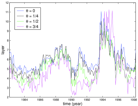
Figure 6: Plots of the weighted minimum risk portfolio layer $l_{\mathbf{P}}(t,\theta)$ for different values of $\theta$.

Thus far, we have only examined the location of stocks in the minimum risk portfolio, for which $\theta=0$. However, we note that as we increase $\theta$ towards unity, portfolio risk as a function of time soon starts behaving very differently from the mean correlation coefficient and normalized tree length as shown in Fig. 6. Consequently, it is no longer useful in describing diversification potential of the market. However, another interesting result is noteworthy: The average weighted portfolio layer $l_{\mathbf{P}}(t,\theta)$ decreases for increasing values of $\theta$. This implies that out of all the possible Markowitz portfolios, the minimum risk portfolio stocks are located furthest away from the central vertex, and as we move towards portfolios with higher expected return, the stocks included in these portfolios are located closer to the central vertex. It may be mentioned that we have not included the weighted portfolio layer for $\theta=1$, as it is not very informative. This is due to the fact that the maximum return portfolio comprises only one asset (the maximum return asset in the current time window) and, therefore, $l_{\mathbf{P}}(t,\theta=1)$ fluctuates wildly as the maximum return asset changes over time.

We believe these results to have potential for practical application. Stocks included in low risk portfolios are consistently located further away from the central node than those included in high risk portfolios. Consequently, the radial distance of a node, i.e. its occupation layer, is meaningful. We conjecture that the location of a company within the cluster reflects its position with regard to internal, or cluster specific, risk. Thus the characterization of stocks by their branch, as well as their location within the branch, would enable us to identify the degree of interchangeability of different stocks in the portfolio. In most cases, we would be able to pick two stocks from different asset tree clusters, but from nearby layers, and interchange them in the portfolio without considerably altering the characteristics of the portfolio. Therefore, dynamic asset trees may facilitate incorporation of subjective judgment in the portfolio optimization problem.

III Summary

We have studied the dynamics of asset trees and applied it to market taxonomy and portfolio analysis. We have noted that the tree evolves over time and the mean occupation layer fluctuates as a function of time, and experiences a downfall at the time of market crisis due to topological changes in the asset tree. For the portfolio analysis, it was found that the stocks included in the minimum risk portfolio tend to lie on the outskirts of the asset tree: on average the weighted portfolio layer can be almost one and a half levels higher, or further away from the central vertex, than the mean occupation layer for window width of four years. Finally, the asset tree can be used as a visualization tool, and even though it is strongly pruned, it still retains all the essential information of the market (starting from the correlations in stock prices) and can be used to add subjective judgement to the portfolio optimization problem.

IV acknowledgements

The author would like to thank all his collaborators, and also the critics for their valuable comments during the lectures given at IPST (Maryland, USA), Bose Institute (Kolkata) and MMV (BHU, Varanasi).

References

- (1) L. Bachelier, Theorie de la Speculation (Gauthier-Villars, Paris, 1900).
- (2) A. Chakraborti and M.S. Santhanam, Int. J. Mod. Physics 16, 1733 (2005).
- (3) R.S. Tsay, Analysis of Financial Time Series (John Wiley, New York, 2002).
- (4) R.N. Mantegna and H.E. Stanley, An Introduction to Econophysics (Cambridge University Press, New York, 2000).
- (5) J.-P. Onnela, Taxonomy of Financial Assets (M. Sc. Thesis, Helsinki University of Technology, Finland, 2002).
- (6) J.-P. Onnela, A. Chakraborti, K. Kaski and J. Kertesz, Phys. Rev. E 68, 056110 (2003).
- (7) R. N. Mantegna, Eur. Phys. J. B 11, 193 (1999).
- (8) J.-P. Onnela, A. Chakraborti, K. Kaski and J. Kertesz, Physica A 324, 247 (2002).
- (9) http://www.forbes.com/ (2003).
- (10) J.-P. Onnela, A. Chakraborti, K. Kaski and J. Kertesz, Eur. Phys. J. B 30, 285 (2002).
- (11) http://www.lce.hut.fi/ jonnela/ (2003).