A method for incorporating systematic errors into branching ratio limits which are not obtained from a simple counting analysis has been suggested by Mark Convery [2]. The derivation makes some approximations which are not necessarily valid. This note presents the full solution as an alternative. The basic idea is a simple extension of the Cousins and Highland philosophy [3]. Before systematics are considered, an analysis using a maximum likelihood fit returns a central value for the branching ratio $(\hat{B})$ and a statistical error $(\sigma_{B})$. The likelihood function is

$$p(B)\propto\exp{\!\left[\frac{-(B-\hat{B})^{2}}{2\sigma_{B}^{2}}\right]}.$$ (1)

Following the Convery notation, we associate $\hat{S}$ with the nominal efficiency and $\sigma_{S}$ as the (Gaussian) error on the efficiency. Adding the uncertainty on the efficiency changes the likelihood to:

$$p(B)\propto\int_{0}^{1}\exp{\!\left[\frac{-(SB/\hat{S}-\hat{B})^{2}}{2\sigma_{B}^{2}}\right]}\exp{\!\left[\frac{-(S-\hat{S})^{2}}{2\sigma_{s}^{2}}\right]}d\!S.$$ (2)

From Mathematica${}^{\textrm{\textregistered}}$, the integral in Eq. 2 is:

$$\sqrt{\frac{\pi}{2}}\frac{\hat{S}}{\sqrt{\frac{B^{2}}{\sigma_{B}^{2}}+\frac{\hat{S}^{2}}{\sigma_{S}^{2}}}}\exp{\!\!\left[\!\frac{-(B-\hat{B})^{2}}{2\left(\frac{B^{2}\sigma_{S}^{2}}{\hat{S}^{2}}+\sigma_{B}^{2}\right)}\!\right]}\!\left\{\textrm{erf}\!\left[\!\frac{\hat{S}\left(\sigma_{B}^{2}+\frac{B\hat{B}\sigma_{S}^{2}}{\hat{S}^{2}}\right)}{\sqrt{2}\sigma_{B}\sigma_{S}\sqrt{\frac{B^{2}\sigma_{S}^{2}}{\hat{S}^{2}}+\sigma_{B}^{2}}}\!\right]-\textrm{erf}\!\left[\!\frac{(\hat{S}-1)\sigma_{B}^{2}-B\sigma_{S}^{2}\left(\frac{b}{\hat{S}^{2}}-\frac{\hat{B}}{\hat{S}}\right)}{\sqrt{2}\sigma_{B}\sigma_{S}\sqrt{\frac{B^{2}\sigma_{S}^{2}}{\hat{S}^{2}}+\sigma_{B}^{2}}}\!\right]\!\right\}\!.$$

Removing unimportant multiplicative constants and changing variables from $\sigma_{S}$ to $\sigma_{\epsilon}\equiv\sigma_{S}/\hat{S}$ gives:

$$p(B)\propto\frac{1}{\sqrt{\frac{B^{2}}{\sigma_{B}^{2}}+\frac{1}{\sigma_{\epsilon}^{2}}}}\exp{\!\!\left[\!\frac{-(B-\hat{B})^{2}}{2(B^{2}\sigma_{\epsilon}^{2}+\sigma_{B}^{2})}\!\right]}\!\left\{\textrm{erf}\!\left[\!\frac{B\hat{B}\sigma_{\epsilon}^{2}+\sigma_{B}^{2}}{\sqrt{2}\sigma_{\epsilon}\sigma_{B}\sqrt{B^{2}\sigma_{\epsilon}^{2}+\sigma_{B}^{2}}}\!\right]-\textrm{erf}\!\left[\!\frac{(\hat{S}-1)\sigma_{B}^{2}-B\sigma_{\epsilon}^{2}(B-\hat{B}\hat{S})}{\sqrt{2}\hat{S}\sigma_{\epsilon}\sigma_{B}\sqrt{B^{2}\sigma_{\epsilon}^{2}+\sigma_{B}^{2}}}\!\right]\!\right\}\!.$$ (3)

It turns out that as long as the efficiency $\hat{S}$ is sufficiently small (generally less than 10% but dependent on other parameters), the second erf term evaluates to $-1$ and the dependence on the efficiency is removed.

The solution to the integral presented by Convery (for $\sigma_{S}\ll\hat{S}$) can be written as:

$$p(B)\propto\frac{1}{\sqrt{\frac{B^{2}}{\sigma_{B}^{2}}+\frac{1}{\sigma_{\epsilon}^{2}}}}\exp{\!\left[\frac{-(B-\hat{B})^{2}}{2\left(B^{2}\sigma_{\epsilon}^{2}+\sigma_{B}^{2}\right)}\right]}.$$ (4)

The differences between Eq. 3 and Eq. 4 are the two erf terms in Eq. 3. The first erf term affects the tails of the distribution and becomes increasingly important as $\sigma_{\epsilon}$ increases. The second erf term affects the peak position and is important when $\hat{S}\pm\sigma_{S}$ is not easily contained in the region $\{0,1\}$. Or, for a fixed $\sigma_{\epsilon}$, when $\hat{S}$ approaches unity. Next we compare the two results after modifying Equations 4 and 3 to normalize them such that $p(B=\hat{B})=1$.

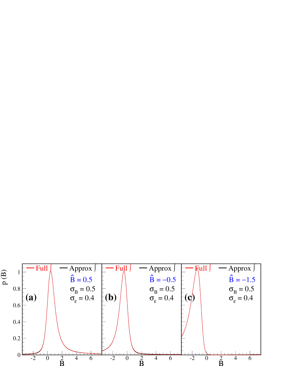
First we check the effect for relatively large $\sigma_{\epsilon}$ and small $\hat{S}$ for which the first erf term becomes important. Each plot of Figure 1 shows a comparison between the full solution in red and the approximate solution in black. There is very little discernible difference between the two solutions. The different plots show results for $\hat{B}=0.5$, $\hat{B}=-0.5$, and $\hat{B}=-1.5$. 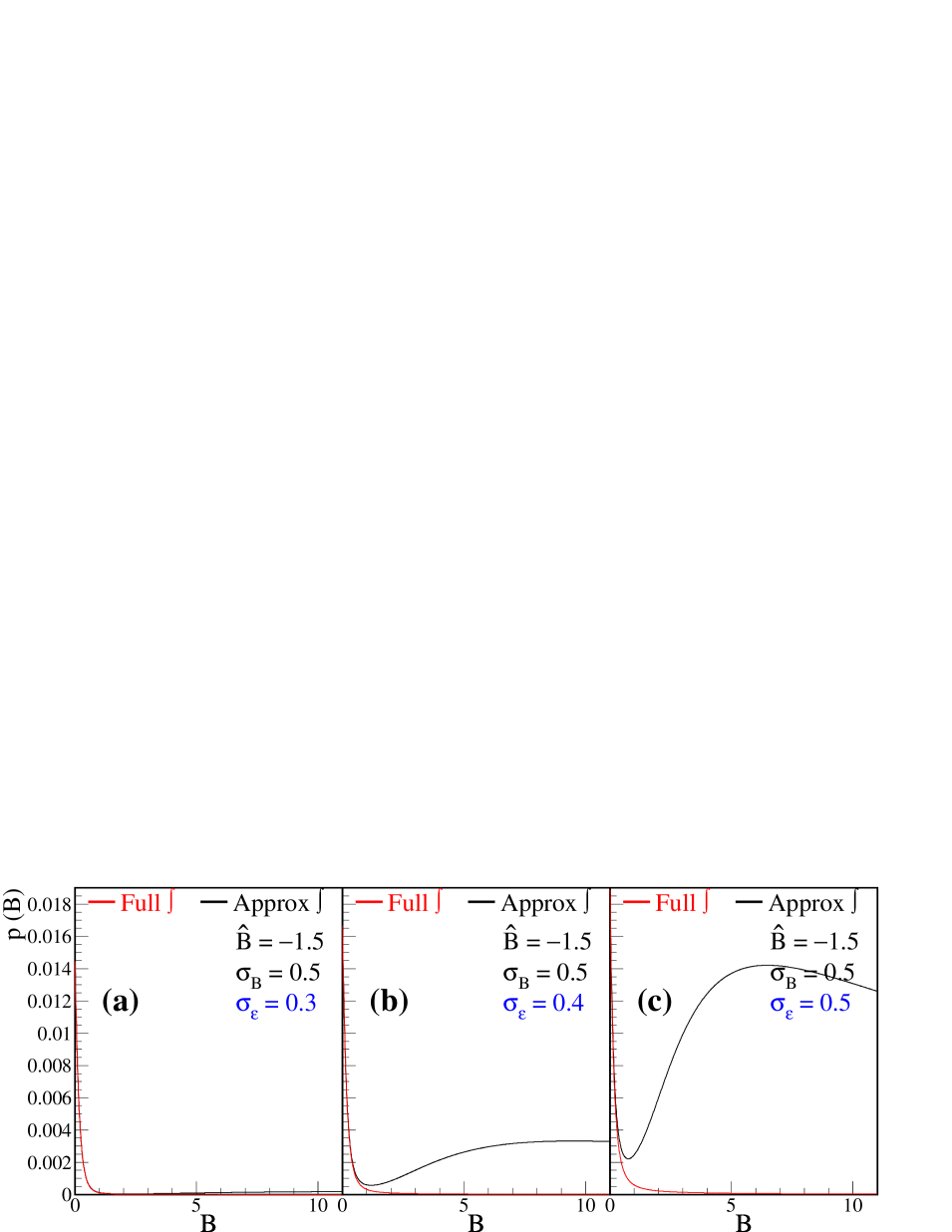To set an upper limit, one often integrates the probability over the physical region only $(B>0)$. Figure 2 shows the results for $p(B)$ over the range $B\in\{0,17\}$ for the case of $\hat{B}=-1.5$ and $\sigma_{B}=0.5$ which corresponds to a $3\sigma$ negative fluctuation. In this case clear differences between the full solution (in red) and the approximate solution (black) can be seen for $\sigma_{\epsilon}\geq 0.3$. Note that Fig. 1(a) and Fig. 2(b) show the same curves, only the range has changed. Clearly an attempt to find an upper limit by integrating the area under the approximate solution is problematic for all the cases shown in Fig. 2. Conversely, the full solution finds an acceptable upper limit.

Figure 1: Each plot shows a comparison of the approximate solution given by Eq. 4 in black to the full solution given by Eq. 3 in red. For all plots, $\sigma_{B}=0.5$, $\sigma_{\epsilon}=0.4$, and $\hat{S}=\epsilon=0.1$. The three plots show results for $\hat{B}=0.5$, $\hat{B}=-0.5$, and $\hat{B}=-1.5$.

Figure 2: Each plot shows a comparison of the approximate solution given by Eq. 4 in black to the full solution given by Eq. 3 in red. For all plots, $\sigma_{B}=0.5$, $\hat{B}=-1.5$, and $\hat{S}=\epsilon=0.1$. The three plots show results for $\sigma_{\epsilon}=0.3$, $\sigma_{\epsilon}=0.4$, and $\sigma_{\epsilon}=0.5$. In this case, the full solution is indistinguishable from the full solution with the second erf term replaced by $-1$.

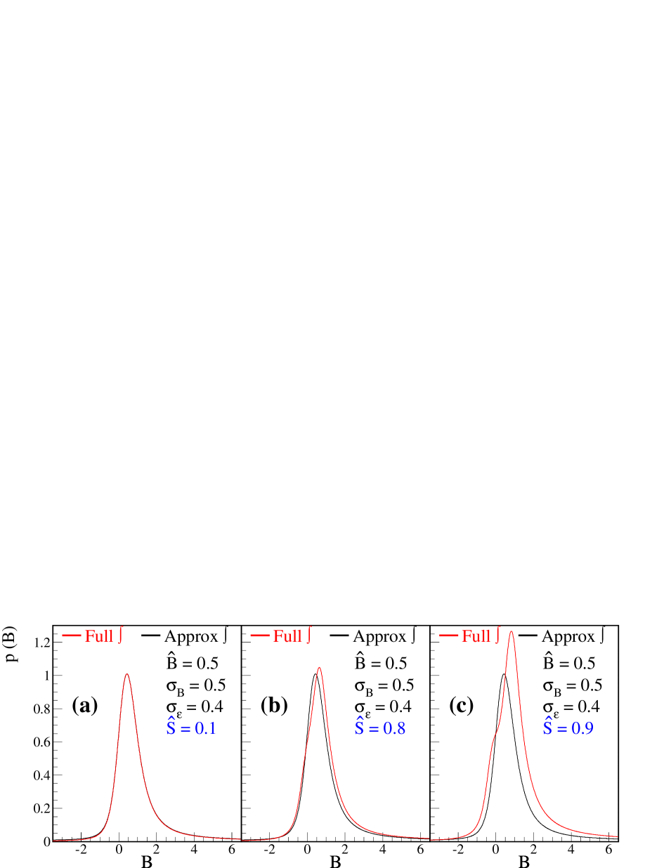
Second we check the effect of the second erf term of Eq. 3 which is important when the integration of efficiency from $0$ to $1$ in Eq. 2 cuts off a significant part of the Gaussian defined by $\hat{S}\pm\sigma_{S}=\hat{S}\pm\sigma_{\epsilon}\hat{S}$. Figure 3(a) is a repeat of Fig. 1(a) on a different scale and again shows little difference between the two methods. Figures 3(b) and 3(c) show the effect of the second erf term as $\hat{S}\rightarrow 1$.

Figure 3: Each plot shows a comparison of the approximate solution given by Eq. 4 in black to the full solution given by Eq. 3 in red. For all plots, $\sigma_{B}=0.5$, $\hat{B}=0.5$, and $\sigma_{\epsilon}=0.4$. The three plots show results for $\hat{S}=\epsilon=0.1$, $\hat{S}=\epsilon=0.8$, and $\hat{S}=\epsilon=0.9$. In this case, the full solution is nearly indistinguishable from the full solution with the first erf term replaced by $+1$.

In conclusion, Eq. 3 provides a more exact and robust implementation of the original suggestion by Convery [2] on incorporating multiplicative systematic uncertainties in branching ratio limits.

References

• [1]
• [2] M. R. Convery, Incorporating Multiplicative Systematic Errors in Branching Ratio Limits, SLAC-TN-03-001, 2003.
• [3] R. D. Cousins and V. L. Highland, Nucl. Instrum. and Meth. A320 (1992) 331.