Coherent thermodynamical modelling of geomaterial reinforced by wire

Abstract

The TexSol is a composite geomaterial : a sand matrix and a wire network reinforcement. For small strains a thermodynamical continuous model of the TexSol including the unilaterality of the wire network is postulated. This model is described by two potentials which depend on some internal variables and a state variable either strain or stress tensor (the choice of this last one gives two different ways of identification). The TexSol continuous model is implemented in a finite element code to recover the mechanical behaviour given by discrete elements numerical experiments.

, ,

1 Motivations

1.1 What is the TexSol ?

The civil pieces of work need planed stable floor. The environment configuration often forces civil engineers to raise huge embankments. Moreover, it can be interesting to reinforce them to assure a better embankment mechanical behaviour. A lot of different solutions can be used to reinforce soil but, in this paper, we focus our attention to the TexSol process.

The TexSol, created in 1984 by Leflaive Khay and Blivet from LCPC (Laboratoire Central des Ponts et Chaussées) [12], is a heterogeneous material by mixing sand and wire network. This reinforced material has a better mechanical resistance than the sand without wire. Of course, the TexSol behaviour depends on sand and wire parameters and its frictional angle can be larger than the sand one from $0^{\circ}$ to $10^{\circ}$ [8]. The wire is described by its linear density with a dtex unit ($1\mbox{ dtex}=0,1\mbox{ g}.\mbox{km}^{-1}$), its ponderal content and its stiffness. Classically, the wire density in a TexSol sample is included between $100\mbox{ km}.\mbox{m}^{-3}$ and $200\mbox{ km}.\mbox{m}^{-3}$.

To make a TexSol bank, a machine named “Texsoleuse” is used. It works on throwing sand and, in the same time, injecting wire. The wire is deposed on the free plane of the sand with a random orientation. This machine carries out several passes to raise the bank. The figure 1 is the TexSol microstructure representation.

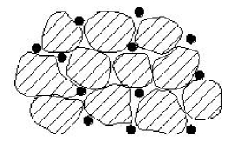
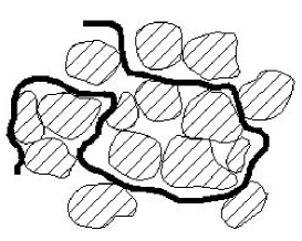
Figure 1: Schematic TexSol sections

In the literature, we find two different continuous modellings. The model suggested in [5] is non local and includes remote interactions (corresponding to the wire effects) but also needs an identification of their parameters using macroscopic experiments. Villard proposes a simpler local model in [20]. This one couples a standard model of sand and an equivalent unilateral elastic stiffness contribution corresponding to the wire network. This last contribution is activated only on the traction directions because of the unilateral behaviour of wire. Our first work is to clearly define thermo-dynamical potentials of the Villard local model with both stress and strain formulations to identify the best-adapted one.

1.2 Assumptions of the continuous local model

To couple the elastic plastic model of the sand and the unilateral elastic model of the wire network, we have to consider some mechanical assumptions, which may be backed up by numerical experiments performed with a discrete elements software [3, 15].

1.2.1 Stress additivity assumption

In this paper, the stress additivity assumption of the sand and the wire network is assumed. Then we write,

$$\mbox{\boldmath{$\sigma$}}_{s}+\mbox{\boldmath{$\sigma$}}_{w}=\mbox{\boldmath{$\sigma$}}\mbox{ ,}$$ (1)

where $\mbox{\boldmath{$\sigma$}}_{s}$, $\mbox{\boldmath{$\sigma$}}_{w}$ and $\sigma$ are respectively the stress second order tensor of the sand, the wire network and the TexSol.

This assumption seems to be coherent with the TexSol quasi-static behaviour. We can get a good approximation of the stress tensor in numerical simulation of 2D granular matter [16] using the Weber stress tensor [1]. This tensor may be non symmetrical if inertial effects are not negligeable. For quasi-static processes this discrete tensor is a good candidate to represent a continuous stress tensor. Moreover we can define such a tensor grain by grain with the Moreau approach [15]. In this way a wire network stress and a sand stress may be computed, to recover by addition the full TexSol stress (in the simulation, the wire is modeled by a chain of beads with unilateral interactions [11]). On a biaxial crushing test we verify the symmetry property even for large deformation as long as the process remains slow.

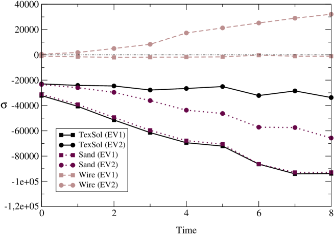
Figure 2: Stress eigen values evolution in the TexSol

The eigenvalues $(\mbox{EV}1,\mbox{EV}2)$ are computed and the contribution of each component of the TexSol are underlined in the figure 2 where the wire network is only in a tensile state ; in the two eigen directions the sand is in compression. This may be also observed on the distribution of force network in the granular sample.

1.2.2 Non sliding assumption

This second assumption is not as evident as the previous one. Although micro slidings occur between sand grains and wire, we assume that at the macroscopic level of the continuum model, the sand network does not slip through the wire network. This assumption can be translated by the equality of the three strain rates,

$$\mbox{\boldmath{$\stackrel{{\scriptstyle\cdot}}{{\varepsilon}}$}}_{s}=\mbox{\boldmath{$\stackrel{{\scriptstyle\cdot}}{{\varepsilon}}$}}_{w}=\mbox{\boldmath{$\stackrel{{\scriptstyle\cdot}}{{\varepsilon}}$}}\mbox{ ,}$$ (2)

where $\mbox{\boldmath{$\varepsilon$}}_{s}$, $\mbox{\boldmath{$\varepsilon$}}_{w}$ and $\varepsilon$ are respectively the strain second order tensor of the sand, the wire network and the TexSol.

We have to be very careful with such a condition and define some validity domains for it. Indeed the limits of this assumption are difficult to quantify and we will restrict the validation of the following continuum model to small strains.

1.3 Role of the wire unilaterality

The wire network contributes to the tensile srtength of the composite material but not to the compression one (cf. figure 2). To model such a behaviour at the macroscopic scale, it is convenient to introduce a unilateral condition in the behaviour law of the wire network. This unilaterality accounts for two microscopic phenomena. The first one is the lack of bending strength of the wire network viewed as a piece of cotton. The second one is the local buckling of short segments. The first aspect is not explicitely taken into account by a unilateral condition at the microscopic scale in our discrete numerical simulation since the chain of beads has no bending strength. The second aspect may be enforced by introducing a unilateral interaction law between two successive beads.

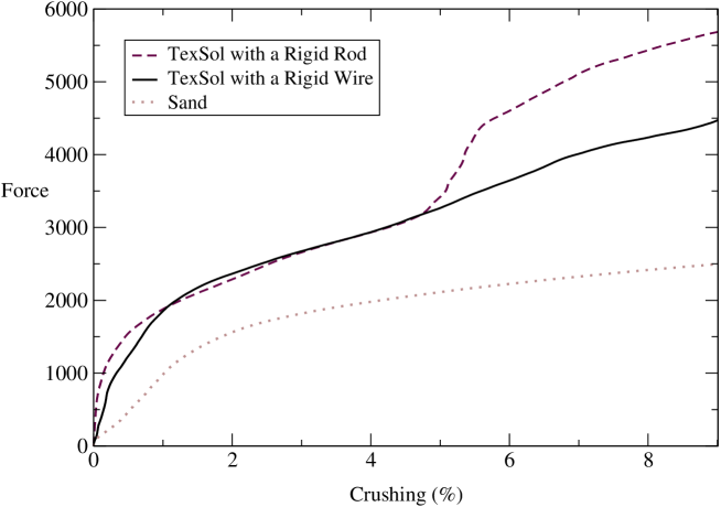
Figure 3: Force / Crushing response with different models

Figure 4: Schematic discrete laws

Such an interaction models an elemental wire between two beads : we denote by “rigid wire”; if not we speak about “rigid rod” (cf. figure 4) for bilateral law between beads. The figure 3 illustrates the difference of global behaviour between both simulation for crushing biaxial test. Until $6$ percents of deformation, the responses are almost identical. For larger deformation the “rigid rod” model leads to a rough increase of rigidity due to the appearance of compression columns in the wire. Such a phenomenon seems not very realistic and is probably issued from a scale effect since the numerical sample is not representative enough of the material. In particular the model of wire with a chain of beads generates non realistic wedges of beads by sand grains.

1.4 Why a strain and stress formulation ?

In this paper, we propose to carry out a thermodynamical study with both strain and stress formulations. The interest of this work is in the identification possibilities of potentials parameters. Indeed, an experimentator making some tests on a sample has only access to the global strain. Our numerical investigations allow us to have access to finer data such as the local stress field throughout the sample. Moreover the global stress tensor over the sample can be deduced by an average.

The post processing of numerical experiments mentioned in §1.2.1 provides precise informations on the stress fields, in the sand and in the wire network. The stress “unilaterality” in the wire is clearly established in the figure 2. This observation could lead us to favour a stress formulation. But the finite element softwares are essentially developed using a strain formulation. Consequently we propose, in the following study, strain formulations easily implementable. Dual stress formulations are provided when they can be analytically deduced by the Legendre – Fenchel transformation.

2 A general thermodynamical framework

In this part, we define potentials written with different state variables. These potentials have to check the Clausius–Duhem inequality to be thermodynamically admissible.

2.1 Strain versus stress approach in thermodynamics

This work must be as exhaustive as possible, while passing from unspecified state variables to its dual. We thus use the Legendre–Fenchel transformation [14], to carry out our study with both strain and stress formulations. Let us write the Clausius–Duhem inequality where $u$ is the internal energy, $s$ the entropy, $q$ the heat flow and $T$ the temperature,

$$\mbox{\boldmath{$\sigma$}}:\stackrel{{\scriptstyle\cdot}}{{\mbox{\boldmath{$\varepsilon$}}}}-\rho\left(\stackrel{{\scriptstyle\cdot}}{{u}}-T\stackrel{{\scriptstyle\cdot}}{{s}}\right)-\frac{1}{T}q.\bigtriangledown T\geq 0\mbox{ .}$$ (3)

The intrinsic dissipation depends on a state variable $X$ (or its dual $\mbox{\boldmath{$X$}}^{*}$), some internal variables $\alpha=\left\{\alpha_{1},\cdots,\alpha_{p}\right\}$ (each internal variable can be scalar, vectorial or tensorial) and the temperature $T$. It can also be expressed with the free energy $\psi$ or its Legendre–Fenchel transformation $\psi^{*}$ with respect to the state variable $X$,

$$\begin{array}[]{c}\\ \mbox{and }\\ \\ \end{array}\begin{array}[]{l}\begin{array}[]{l}\psi(\mbox{\boldmath{$X$}},\alpha,T)=u(\mbox{\boldmath{$X$}},\alpha,T)-Ts(\mbox{\boldmath{$X$}},\alpha,T)\\ \end{array}\\ \begin{array}[]{ll}\psi^{*}(\mbox{\boldmath{$X$}}^{*},\alpha,T)&=\mathord{\vtop{\halign{#\cr$\hfil\mbox{sup}\hfil$\crcr\kern 1.5pt\nointerlineskip\cr$\hfil\scriptstyle{\mbox{\boldmath{$\scriptstyle{\overline{X}}$}}}\hfil$\crcr\kern 1.5pt\cr}}}\left\{\mbox{\boldmath{$\overline{X}$}}:\mbox{\boldmath{$X$}}^{*}-\psi(\mbox{\boldmath{$\overline{X}$}},\alpha,T)\right\}\\ &=\mbox{\boldmath{$X$}}:\mbox{\boldmath{$X$}}^{*}-\psi(\mbox{\boldmath{$X$}},\alpha,T)\mbox{ ,}\\ \end{array}\\ \end{array}$$

where $X$ is the argument of the supremum. Considering either $X$ or $\mbox{\boldmath{$X$}}^{*}$, we find two expressions of the Clausius–Duhem inequality,

$$\begin{array}[]{c}\mbox{\boldmath{$\sigma$}}:\stackrel{{\scriptstyle\cdot}}{{\mbox{\boldmath{$\varepsilon$}}}}-\rho\left[\frac{\partial\psi}{\partial\mbox{\boldmath{$\scriptstyle{X}$}}}:\stackrel{{\scriptstyle\cdot}}{{\mbox{\boldmath{$X$}}}}+\left(s+\frac{\partial\psi}{\partial T}\right)\stackrel{{\scriptstyle\cdot}}{{T}}+\frac{\partial\psi}{\partial\alpha_{m}}\stackrel{{\scriptstyle\cdot}}{{\alpha}}_{m}\right]-\frac{q}{T}.\bigtriangledown T\geq 0\end{array}\mbox{ ,}$$ (4)

$$\begin{array}[]{rcl}\mbox{\boldmath{$\sigma$}}:\stackrel{{\scriptstyle\cdot}}{{\mbox{\boldmath{$\varepsilon$}}}}-\rho\left[\stackrel{{\scriptstyle\cdot}}{{\mbox{\boldmath{$X$}}}}:\mbox{\boldmath{$X$}}^{*}+\left(\mbox{\boldmath{$X$}}-\frac{\partial\psi^{*}}{\partial\mbox{\boldmath{$\scriptstyle{X}$}}^{\scriptscriptstyle{*}}}\right):\stackrel{{\scriptstyle\cdot}}{{\mbox{\boldmath{$X$}}}}^{*}+\left(s-\frac{\partial\psi^{*}}{\partial T}\right)\stackrel{{\scriptstyle\cdot}}{{T}}-\frac{\partial\psi^{*}}{\partial\alpha_{m}}\stackrel{{\scriptstyle\cdot}}{{\alpha}}_{m}\right]&&\\ -\frac{q}{T}.\bigtriangledown T&\geq&0\mbox{ .}\end{array}$$ (5)

Using the Helmholtz postulate (this last one can be applied with the generalized standard materials assumption [6]) and the previous definitions, we are now able to deduce the state laws,

$$\begin{array}[]{cccc}\mbox{Primal state laws}&&\mbox{Dual state laws}&\\ &&&\\ \mbox{\boldmath{$X$}}^{*}\in\partial_{\mbox{\boldmath{$\scriptstyle{X}$}}}\psi(\mbox{\boldmath{$X$}},\alpha,T)&&\mbox{\boldmath{$X$}}\in\partial_{\mbox{\boldmath{$\scriptstyle{X}$}}^{*}}\psi^{*}(\mbox{\boldmath{$X$}}^{*},\alpha,T)&\\ -s\in\partial_{T}\psi(\mbox{\boldmath{$X$}},\alpha,T)&&s\in\partial_{T}\psi^{*}(\mbox{\boldmath{$X$}}^{*},\alpha,T)&\\ -\frac{1}{\rho}A_{m}\in\partial_{\alpha_{m}}\psi(\mbox{\boldmath{$X$}},\alpha,T)&&\frac{1}{\rho}A_{m}\in\partial_{\alpha_{m}}\psi^{*}(\mbox{\boldmath{$X$}}^{*},\alpha,T)&\mbox{,}\\ \end{array}$$ (6)

where $A_{m}$ is the thermodynamical force associated with $\alpha_{m}$. Formally we use subdifferentials instead of derivatives. If convexity is not required, previous relations still hold using the Clarke subdifferential [2]. Then the primal and dual forms are not necessary equivalent. In the general case, the Clausius–Duhem inequality (4) or (5) can be reduced to a dot product of a vector flow and a vector force,

$${\underbrace{\left[\begin{array}[]{c}\widehat{\mbox{\boldmath{$\sigma$}}}\\ A\\ \bigtriangledown T\end{array}\right]}_{\mbox{force}}}^{T}.\underbrace{\left[\begin{array}[]{c}\stackrel{{\scriptstyle\cdot}}{{\widehat{\mbox{\boldmath{$\varepsilon$}}}}}\\ \stackrel{{\scriptstyle\cdot}}{{\alpha}}\\ -\frac{q}{T}\end{array}\right]}_{\mbox{flow}}\geq 0\qquad\mbox{where }\left\{\begin{array}[]{rcl}\stackrel{{\scriptstyle\cdot}}{{\widehat{\mbox{\boldmath{$\varepsilon$}}}}}&=&\stackrel{{\scriptstyle\cdot}}{{\mbox{\boldmath{$\varepsilon$}}}}\mbox{ or }\stackrel{{\scriptstyle\cdot}}{{\mbox{\boldmath{$\varepsilon$}}}}^{ir}\\ \widehat{\mbox{\boldmath{$\sigma$}}}&=&\mbox{\boldmath{$\sigma$}}^{ir}\mbox{ or }\mbox{\boldmath{$\sigma$}}\end{array}\right.\mbox{ .}$$ (7)

The flow variables have to be related by evolution laws to the force variables. To verify the inequality (7) some assumptions may be added to these relations. It is convenient to introduce a dissipation potential $\varphi$ from which the evolution laws are derived. By duality a force function $\varphi^{*}$ is automatically defined using the Legendre–Fenchel transformation,

$$\begin{array}[]{cccc}\mbox{Primal complementary laws}&&\mbox{Dual complementary laws}&\\ &&&\\ \widehat{\mbox{\boldmath{$\sigma$}}}\in\partial_{\stackrel{{\scriptstyle\cdot}}{{\widehat{\mbox{\boldmath{$\scriptstyle{\varepsilon}$}}}}}}\varphi(\stackrel{{\scriptstyle\cdot}}{{\widehat{\mbox{\boldmath{$\varepsilon$}}}}},\stackrel{{\scriptstyle\cdot}}{{\alpha}},-\frac{q}{T})&&\stackrel{{\scriptstyle\cdot}}{{\widehat{\mbox{\boldmath{$\varepsilon$}}}}}\in\partial_{\widehat{\mbox{\boldmath{$\scriptstyle{\sigma}$}}}}\varphi^{*}(\widehat{\mbox{\boldmath{$\sigma$}}},\stackrel{{\scriptstyle\cdot}}{{\alpha}},-\frac{q}{T})&\\ A\in\partial_{\stackrel{{\scriptstyle\cdot}}{{\alpha}}}\varphi(\stackrel{{\scriptstyle\cdot}}{{\widehat{\mbox{\boldmath{$\varepsilon$}}}}},\stackrel{{\scriptstyle\cdot}}{{\alpha}},-\frac{q}{T})&&-A\in\partial_{\stackrel{{\scriptstyle\cdot}}{{\alpha}}}\varphi^{*}(\widehat{\mbox{\boldmath{$\sigma$}}},\stackrel{{\scriptstyle\cdot}}{{\alpha}},-\frac{q}{T})&\\ \bigtriangledown T\in\partial_{\left(-\frac{q}{T}\right)}\varphi(\stackrel{{\scriptstyle\cdot}}{{\widehat{\mbox{\boldmath{$\varepsilon$}}}}},\stackrel{{\scriptstyle\cdot}}{{\alpha}},-\frac{q}{T})&&-\bigtriangledown T\in\partial_{\left(-\frac{q}{T}\right)}\varphi^{*}(\widehat{\mbox{\boldmath{$\sigma$}}},\stackrel{{\scriptstyle\cdot}}{{\alpha}},-\frac{q}{T})&\mbox{.}\\ \end{array}$$ (8)

To verify the Clausius–Duhem inequality, some assumptions on the dissipation potential are necessary. For simplicity we consider now an isothermal process. The left-hand side of the inequality is reduced to,

$$\widehat{\mbox{\boldmath{$\sigma$}}}:\stackrel{{\scriptstyle\cdot}}{{\widehat{\mbox{\boldmath{$\varepsilon$}}}}}+A\stackrel{{\scriptstyle\cdot}}{{\alpha}}\;=\frac{\partial\varphi}{\partial\stackrel{{\scriptstyle\cdot}}{{\widehat{\mbox{\boldmath{$\varepsilon$}}}}}}:\stackrel{{\scriptstyle\cdot}}{{\widehat{\mbox{\boldmath{$\varepsilon$}}}}}+\frac{\partial\varphi}{\partial\stackrel{{\scriptstyle\cdot}}{{\alpha}}}\stackrel{{\scriptstyle\cdot}}{{\alpha}}\;=\left\langle\partial\varphi(\stackrel{{\scriptstyle\cdot}}{{\widehat{\mbox{\boldmath{$\varepsilon$}}}}},\stackrel{{\scriptstyle\cdot}}{{\alpha}}),\left(\stackrel{{\scriptstyle\cdot}}{{\widehat{\mbox{\boldmath{$\varepsilon$}}}}},\stackrel{{\scriptstyle\cdot}}{{\alpha}}\right)\right\rangle$$

and the primal state laws are summarized in $\left(\widehat{\mbox{\boldmath{$\sigma$}}},A\right)\in\partial\varphi(\stackrel{{\scriptstyle\cdot}}{{\widehat{\mbox{\boldmath{$\varepsilon$}}}}},\stackrel{{\scriptstyle\cdot}}{{\alpha}})$. $\varphi$ being a separately convex function, with a convex analysis characterisation of the subdifferential we write,

$$\forall\left(\mbox{\boldmath{$x$}},y\right)\quad\varphi(\stackrel{{\scriptstyle\cdot}}{{\widehat{\mbox{\boldmath{$\varepsilon$}}}}},\stackrel{{\scriptstyle\cdot}}{{\alpha}})-\varphi(\mbox{\boldmath{$x$}},y)\leq\left\langle\left(\stackrel{{\scriptstyle\cdot}}{{\widehat{\mbox{\boldmath{$\varepsilon$}}}}},\stackrel{{\scriptstyle\cdot}}{{\alpha}}\right)-\left(\mbox{\boldmath{$x$}},y\right),\left(\widehat{\mbox{\boldmath{$\sigma$}}},A\right)\right\rangle\mbox{ .}$$

Moreover, if $\varphi$ is minimum in $\left(\mbox{\boldmath{$0$}},0\right)$, the Clausius–Duhem inequality is then verified [18],

$$\widehat{\mbox{\boldmath{$\sigma$}}}:\stackrel{{\scriptstyle\cdot}}{{\widehat{\mbox{\boldmath{$\varepsilon$}}}}}+A\stackrel{{\scriptstyle\cdot}}{{\alpha}}\;\geq\varphi(\stackrel{{\scriptstyle\cdot}}{{\widehat{\mbox{\boldmath{$\varepsilon$}}}}},\stackrel{{\scriptstyle\cdot}}{{\alpha}})-\varphi(\mbox{\boldmath{$0$}},0)\geq 0\mbox{ .}$$

Similar properties are required for $\varphi^{*}$ to recover the Clausius–Duhem inequality. Generally we distinguish the reversible and irreversible parts of the transformation. We thus postulate an additive decomposition for both reversible and irreversible parts of the strain tensor $\mbox{\boldmath{$\varepsilon$}}=\mbox{\boldmath{$\varepsilon$}}^{r}+\mbox{\boldmath{$\varepsilon$}}^{ir}$ and the stress tensor $\mbox{\boldmath{$\sigma$}}=\mbox{\boldmath{$\sigma$}}^{r}+\mbox{\boldmath{$\sigma$}}^{ir}$. The reversible / irreversible splitting of $\sigma$ is less classical. To illustrate its interest, remark that eventual residual stresses may be accounted for in the irreversible part.

At this stage we have to choose the external state variable $X$ for the strain formulation and consequently $\mbox{\boldmath{$X$}}^{*}$ for the stress formulation. It is usual to consider for $X$ the total strain tensor $\varepsilon$. By the way the reversible stress $\mbox{\boldmath{$\sigma$}}^{r}$ appears in the state law and becomes the state variable in the dual stress formulation. But we can also use the reversible strain part $\mbox{\boldmath{$\varepsilon$}}^{r}$ and deduce the full stress tensor $\sigma$ as the dual state variable (cf. table 1).

State variable : $\mbox{\boldmath{$\varepsilon$}}^{r}$		State variable : $\sigma$
$\mbox{\boldmath{$\sigma$}}:\stackrel{{\scriptstyle\cdot}}{{\mbox{\boldmath{$\varepsilon$}}}}^{ir}+A_{m}\stackrel{{\scriptstyle\cdot}}{{\alpha}}_{m}-\frac{q}{T}\bigtriangledown T\geq 0$		$\stackrel{{\scriptstyle\cdot}}{{\mbox{\boldmath{$\varepsilon$}}}}^{ir}:\mbox{\boldmath{$\sigma$}}+A_{m}\stackrel{{\scriptstyle\cdot}}{{\alpha}}_{m}-\frac{q}{T}\bigtriangledown T\geq 0$
free energy : $\psi$	Dissipation potential : $\varphi$	Free enthalpy : $\psi^{*}$	Force function : $\varphi^{*}$
$\frac{1}{\rho}\mbox{\boldmath{$\sigma$}}\in\partial_{\mbox{\boldmath{$\scriptstyle{\varepsilon}$}}^{r}}\psi$	$\mbox{\boldmath{$\sigma$}}\in\partial_{\mbox{\boldmath{$\scriptstyle{\stackrel{{\scriptstyle\cdot}}{{\varepsilon}}}$}}^{ir}}\varphi$	$\frac{1}{\rho}\mbox{\boldmath{$\varepsilon$}}^{r}\in\partial_{\mbox{\boldmath{$\scriptstyle{\sigma}$}}}\psi^{*}$	$\mbox{\boldmath{$\stackrel{{\scriptstyle\cdot}}{{\varepsilon}}$}}^{ir}\in\partial_{\mbox{\boldmath{$\scriptstyle{\sigma}$}}}\varphi^{*}$
$-s\in\partial_{T}\psi$	$A_{m}\in\partial_{\stackrel{{\scriptstyle\cdot}}{{\alpha}}_{m}}\varphi$	$s\in\partial_{T}\psi^{*}$	$-A_{m}\in\partial_{\stackrel{{\scriptstyle\cdot}}{{\alpha}}_{m}}\varphi^{*}$
$-\frac{1}{\rho}A_{m}\in\partial_{\alpha_{m}}\psi$	$\bigtriangledown T\in\partial_{\scriptscriptstyle{\left(-\frac{q}{T}\right)}}\varphi$	$\frac{1}{\rho}A_{m}\in\partial_{\alpha_{m}}\psi^{*}$	$-\bigtriangledown T\in\partial_{\scriptscriptstyle{\left(-\frac{q}{T}\right)}}\varphi^{*}$
State variable : $\varepsilon$		State variable : $\mbox{\boldmath{$\sigma$}}^{r}$
$\mbox{\boldmath{$\sigma$}}^{ir}:\stackrel{{\scriptstyle\cdot}}{{\mbox{\boldmath{$\varepsilon$}}}}+A_{m}\stackrel{{\scriptstyle\cdot}}{{\alpha}}_{m}-\frac{q}{T}\bigtriangledown T\geq 0$		$\stackrel{{\scriptstyle\cdot}}{{\mbox{\boldmath{$\varepsilon$}}}}:\mbox{\boldmath{$\sigma$}}^{ir}+A_{m}\stackrel{{\scriptstyle\cdot}}{{\alpha}}_{m}-\frac{q}{T}\bigtriangledown T\geq 0$
Free energy : $\psi$	Dissipation potential : $\varphi$	Free enthalpy : $\psi^{*}$	Force function : $\varphi^{*}$
$\frac{1}{\rho}\mbox{\boldmath{$\sigma$}}^{r}\in\partial_{\mbox{\boldmath{$\scriptstyle{\varepsilon}$}}}\psi$	$\mbox{\boldmath{$\sigma$}}^{ir}\in\partial_{\stackrel{{\scriptstyle\cdot}}{{\mbox{\boldmath{$\scriptstyle{\varepsilon}$}}}}}\varphi$	$\frac{1}{\rho}\mbox{\boldmath{$\varepsilon$}}\in\partial_{\mbox{\boldmath{$\scriptstyle{\sigma}$}}^{r}}\psi^{*}$	$\stackrel{{\scriptstyle\cdot}}{{\mbox{\boldmath{$\varepsilon$}}}}\in\partial_{\mbox{\boldmath{$\scriptstyle{\sigma}$}}^{ir}}\varphi^{*}$
$-s\in\partial_{T}\psi$	$A_{m}\in\partial_{\stackrel{{\scriptstyle\cdot}}{{\alpha}}_{m}}\varphi$	$s\in\partial_{T}\psi^{*}$	$-A_{m}\in\partial_{\stackrel{{\scriptstyle\cdot}}{{\alpha}}_{m}}\varphi^{*}$
$-\frac{1}{\rho}A_{m}\in\partial_{\alpha_{m}}\psi$	$\bigtriangledown T\in\partial_{\scriptscriptstyle{\left(-\frac{q}{T}\right)}}\varphi$	$\frac{1}{\rho}A_{m}\in\partial_{\alpha_{m}}\psi^{*}$	$-\bigtriangledown T\in\partial_{\scriptscriptstyle{\left(-\frac{q}{T}\right)}}\varphi^{*}$

Table 1: Strain versus stress formulations

The first column expresses the primal model using $\mbox{\boldmath{$\varepsilon$}}^{r}$ or $\varepsilon$ as state variable. The second one provides the corresponding dual formulations.

2.2 1D model of reinforced geomaterial

Let us apply previous results to a rheological 1D model of TexSol taking into account the wire unilaterality.

2.2.1 Strain formulation

We choose to superpose a classical 1D model of elasto-plasticity with hardening for sand [13] and a 1D unilateral model of elasticity for wire. We thus propose the two potentials $\psi$ (free energy) and $\varphi$ (dissipation potential) depending on the external state variable $\varepsilon$ and on the internal one $\varepsilon_{2}$ as shown in the figure 5,

Figure 5: Rheological TexSol diagram

$$\psi\left(\varepsilon,\varepsilon_{2}\right)=\left\{\begin{array}[]{ll}\psi_{1}(\varepsilon,\varepsilon_{2})&\quad\mbox{if }\varepsilon\in C_{1}\\ \psi_{2}(\varepsilon,\varepsilon_{2})&\quad\mbox{if }\varepsilon\in C_{2}\\ \end{array}\right.\mbox{ ,}$$ (9)

$$\varphi(\stackrel{{\scriptstyle\cdot}}{{\varepsilon}},\stackrel{{\scriptstyle\cdot}}{{\varepsilon_{2}}})=\sigma_{0}\left|\stackrel{{\scriptstyle\cdot}}{{\varepsilon_{2}}}\right|\mbox{ ,}$$ (10)

where $\begin{array}[]{l}\psi_{1}(\varepsilon,\varepsilon_{2})=\frac{1}{2}K_{w}\varepsilon^{2}+\frac{1}{2}K_{s}\left(\varepsilon-\varepsilon_{2}\right)^{2}+\frac{1}{2}H{\varepsilon_{2}}^{2}\\ \psi_{2}(\varepsilon,\varepsilon_{2})=\frac{1}{2}K_{s}\left(\varepsilon-\varepsilon_{2}\right)^{2}+\frac{1}{2}H{\varepsilon_{2}}^{2}\\ \end{array}$, $\begin{array}[]{l}C_{1}=\left\{\varepsilon\in\mathbbm{R}\left|\varepsilon\geq 0\right.\right\}\\ C_{2}=\left\{\varepsilon\in\mathbbm{R}\left|\varepsilon\leq 0\right.\right\}\\ \end{array}$ and $\sigma_{0}$ the stress threshold. According to the table 1 the state and complementary laws are derived,

$\quad\begin{array}[]{l}\mbox{State laws}\\ \sigma^{r}=\frac{\partial\psi}{\partial\varepsilon}=K_{w}\langle\varepsilon\rangle+K_{s}\left(\varepsilon-\varepsilon_{2}\right)\mbox{ , }A=-\frac{\partial\psi}{\partial\varepsilon_{2}}=K_{s}\left(\varepsilon-\varepsilon_{2}\right)-H\varepsilon_{2}\\ \end{array}$

$\quad\begin{array}[]{l}\mbox{Complementary laws}\\ \sigma^{ir}=\frac{\partial\varphi}{\partial\stackrel{{\scriptstyle\cdot}}{{\varepsilon}}}=0\mbox{ , }A\in\partial_{\stackrel{{\scriptstyle\cdot}}{{\varepsilon_{2}}}}\varphi=\left\{\begin{array}[]{ll}\left\{sign(\stackrel{{\scriptstyle\cdot}}{{\varepsilon_{2}}})\sigma_{0}\right\}&\quad\mbox{if }\stackrel{{\scriptstyle\cdot}}{{\varepsilon_{2}}}\in\mathbbm{R}^{*}\\ \left[-\sigma_{0},\sigma_{0}\right]&\quad\mbox{if }\stackrel{{\scriptstyle\cdot}}{{\varepsilon_{2}}}=0\end{array}\right.\mbox{ ,}\\ \end{array}$

where $\langle\varepsilon\rangle=\mbox{max}(0,\varepsilon)$, the non negative part of $\varepsilon$.

2.2.2 Stress formulation

To determine the stress formulation, we have to calculate the Legendre–Fenchel transformations of $\psi$ and $\varphi$ which are not always analytically accessible. However we can use the following general result convenient for piecewise smooth functions.

Proposition 1

Consider a non overlapping splitting ${\left(C_{i}\right)}_{i=1,n}$ of the strain space $\mathbbm{R}^{3\times 3}$, $\bigcup_{i=1}^{n}C_{i}=\mathbbm{R}^{3\times 3}$, $C_{i}$ close convex cone with $\mbox{mes}(C_{i}\cap C_{j})=0$, $i\neq j$. If $\psi(\mbox{\boldmath{$\varepsilon$}})$ is piecewise defined by $\psi(\mbox{\boldmath{$\varepsilon$}})=\psi_{i}(\mbox{\boldmath{$\varepsilon$}})$ if $\mbox{\boldmath{$\varepsilon$}}\in C_{i}\mbox{, }i=1,\dots,n$ then

$$\psi^{*}(\mbox{\boldmath{$\sigma$}})=\mathord{\vtop{\halign{#\cr$\hfil\mbox{sup}\hfil$\crcr\kern 1.5pt\nointerlineskip\cr$\hfil\scriptstyle{i}\hfil$\crcr\kern 1.5pt\cr}}}\left\{\left(\psi_{i}^{*}\bigtriangledown\textup{I}_{C_{i}^{\circ}}\right)(\mbox{\boldmath{$\sigma$}})\right\}\mbox{ .}$$

Proof : Let recall the definition of inf-convolution of two functions $f$ and $g$ [14], the indicator function of a convex set $A$ and the polar cone $C^{\circ}$ of $C$,

$$\begin{array}[]{l}\circ\quad\left(f\bigtriangledown g\right)(\varepsilon)=\mathord{\vtop{\halign{#\cr$\hfil\mbox{inf}\hfil$\crcr\kern 1.5pt\nointerlineskip\cr$\hfil\scriptstyle{\varepsilon=\varepsilon_{1}+\varepsilon_{2}}\hfil$\crcr\kern 1.5pt\cr}}}\{f(\varepsilon_{1})+f(\varepsilon_{2})\}\\ \circ\quad\textup{I}_{A}(\varepsilon)=\left\{\begin{array}[]{cl}0&\mbox{ if }\varepsilon\in A\\ +\infty&\mbox{ if }\varepsilon\not\in A\\ \end{array}\right.\\ \circ\quad C^{\circ}=\left\{\mbox{\boldmath{$\sigma$}}\left|\mbox{\boldmath{$\varepsilon$}}:\mbox{\boldmath{$\sigma$}}\leq 0\mbox{ , }\forall\mbox{\boldmath{$\varepsilon$}}\in C\right.\right\}\end{array}$$

According to classical rules of convex analysis,

$$\begin{array}[]{rcl}\psi^{*}(\mbox{\boldmath{$\sigma$}})&=&\mathord{\vtop{\halign{#\cr$\hfil\mbox{sup}\hfil$\crcr\kern 1.5pt\nointerlineskip\cr$\hfil\scriptstyle{\mbox{\boldmath{$\scriptstyle{\overline{\varepsilon}}$}}}\hfil$\crcr\kern 1.5pt\cr}}}\left\{\mbox{\boldmath{$\sigma$}}:\mbox{\boldmath{$\overline{\varepsilon}$}}-\mathord{\vtop{\halign{#\cr$\hfil\mbox{inf}\hfil$\crcr\kern 1.5pt\nointerlineskip\cr$\hfil\scriptstyle{i}\hfil$\crcr\kern 1.5pt\cr}}}\left\{\psi_{i}(\mbox{\boldmath{$\overline{\varepsilon}$}})+\textup{I}_{C_{i}}(\mbox{\boldmath{$\overline{\varepsilon}$}})\right\}\right\}\\ &=&\mathord{\vtop{\halign{#\cr$\hfil\mbox{sup}\hfil$\crcr\kern 1.5pt\nointerlineskip\cr$\hfil\scriptstyle{i}\hfil$\crcr\kern 1.5pt\cr}}}\left\{\mathord{\vtop{\halign{#\cr$\hfil\mbox{sup}\hfil$\crcr\kern 1.5pt\nointerlineskip\cr$\hfil\scriptstyle{\mbox{\boldmath{$\scriptstyle{\overline{\varepsilon}}$}}}\hfil$\crcr\kern 1.5pt\cr}}}\left\{\mbox{\boldmath{$\sigma$}}:\mbox{\boldmath{$\overline{\varepsilon}$}}-\psi_{i}(\mbox{\boldmath{$\overline{\varepsilon}$}})-\textup{I}_{C_{i}}(\mbox{\boldmath{$\overline{\varepsilon}$}})\right\}\right\}\\ &=&\mathord{\vtop{\halign{#\cr$\hfil\mbox{sup}\hfil$\crcr\kern 1.5pt\nointerlineskip\cr$\hfil\scriptstyle{i}\hfil$\crcr\kern 1.5pt\cr}}}\left\{\left(\psi_{i}+\textup{I}_{C_{i}}\right)^{*}(\mbox{\boldmath{$\sigma$}})\right\}\\ &=&\mathord{\vtop{\halign{#\cr$\hfil\mbox{sup}\hfil$\crcr\kern 1.5pt\nointerlineskip\cr$\hfil\scriptstyle{i}\hfil$\crcr\kern 1.5pt\cr}}}\left\{\left(\psi_{i}^{*}\bigtriangledown\textup{I}_{C_{i}^{\circ}}\right)(\mbox{\boldmath{$\sigma$}})\right\}\mbox{ .}\\ \end{array}$$

For the 1D model the splitting into two half spaces is obvious and the analytical forms of conjugate functions from (9) are reachable,

$$\begin{array}[]{ll}\psi^{*}_{1}(\sigma^{r},\varepsilon_{2})=\frac{\left(\sigma^{r}+K_{s}\varepsilon_{2}\right)^{2}}{2\left(K_{w}+K_{s}\right)}-\frac{\left(K_{s}+H\right){\varepsilon_{2}}^{2}}{2}&\mbox{ , }C_{1}^{\circ}=\left\{\sigma\in\mathbbm{R}\left|\sigma\leq 0\right.\right\}\\ \psi^{*}_{2}(\sigma^{r},\varepsilon_{2})=\frac{\left(\sigma^{r}+K_{s}\varepsilon_{2}\right)^{2}}{2K_{s}}-\frac{\left(K_{s}+H\right){\varepsilon_{2}}^{2}}{2}&\mbox{ , }C_{2}^{\circ}=\left\{\sigma\in\mathbbm{R}\left|\sigma\geq 0\right.\right\}\mbox{ .}\\ \end{array}$$

Using the proposition 1, we obtain successively,

$$\begin{array}[]{l}\psi_{1}^{*}\bigtriangledown\textup{I}_{C_{1}^{\circ}}=\left\{\begin{array}[]{ll}-\frac{\left(K_{s}+H\right){\varepsilon_{2}}^{2}}{2}&\mbox{if }\scriptstyle{\sigma^{r}+K_{s}\varepsilon_{2}\leq 0}\\ \frac{\left(\sigma^{r}+K_{s}\varepsilon_{2}\right)^{2}}{2\left(K_{w}+K_{s}\right)}-\frac{\left(K_{s}+H\right){\varepsilon_{2}}^{2}}{2}&\mbox{if }\scriptstyle{\sigma^{r}+K_{s}\varepsilon_{2}\geq 0}\\ \end{array}\right.\\ \psi_{2}^{*}\bigtriangledown\textup{I}_{C_{2}^{\circ}}=\left\{\begin{array}[]{ll}-\frac{\left(K_{s}+H\right){\varepsilon_{2}}^{2}}{2}&\mbox{if }\scriptstyle{\sigma^{r}+K_{s}\varepsilon_{2}\geq 0}\\ \frac{\left(\sigma^{r}+K_{s}\varepsilon_{2}\right)^{2}}{2K_{s}}-\frac{\left(K_{s}+H\right){\varepsilon_{2}}^{2}}{2}&\mbox{if }\scriptstyle{\sigma^{r}+K_{s}\varepsilon_{2}\leq 0}\mbox{ .}\\ \end{array}\right.\\ \end{array}$$

Finally,

$$\psi^{*}(\sigma^{r},\varepsilon_{2})=\left\{\begin{array}[]{ll}\frac{\left(\sigma^{r}+K_{s}\varepsilon_{2}\right)^{2}}{2\left(K_{w}+K_{s}\right)}-\frac{\left(K_{s}+H\right){\varepsilon_{2}}^{2}}{2}&\mbox{ if }\sigma^{r}+K_{s}\varepsilon_{2}\geq 0\\ \frac{\left(\sigma^{r}+K_{s}\varepsilon_{2}\right)^{2}}{2K_{s}}-\frac{\left(K_{s}+H\right){\varepsilon_{2}}^{2}}{2}&\mbox{ if }\sigma^{r}+K_{s}\varepsilon_{2}\leq 0\\ \end{array}\right.\mbox{ .}\\$$ (11)

The Legendre–Fenchel transformation of the dissipation potential is computed classically from (10),

$$\varphi^{*}(\sigma^{ir},\stackrel{{\scriptstyle\cdot}}{{\varepsilon_{2}}})=\textup{I}_{\{0\}}(\sigma^{ir})-\sigma_{0}\left|\stackrel{{\scriptstyle\cdot}}{{\varepsilon_{2}}}\right|\mbox{ .}$$ (12)

We implicitely get from the equation (12) : $\sigma^{ir}=0$. The state and complementary laws in the stress formulation are straightforward derived,

$\quad\begin{array}[]{l}\mbox{State laws}\\ \varepsilon=\frac{\partial\psi^{*}}{\partial\sigma^{r}}(\sigma^{ir},\varepsilon_{2})=\left\{\begin{array}[]{ll}\frac{\sigma^{r}+K_{s}\varepsilon_{2}}{K_{w}+K_{s}}&\mbox{\scriptsize{if }}\scriptstyle{\sigma^{r}+K_{s}\varepsilon_{2}\geq 0}\\ \frac{\sigma^{r}+K_{s}\varepsilon_{2}}{K_{s}}&\mbox{\scriptsize{if }}\scriptstyle{\sigma^{r}+K_{s}\varepsilon_{2}\leq 0}\\ \end{array}\right.\\ A=\frac{\partial\psi^{*}}{\partial\varepsilon_{2}}(\sigma^{ir},\varepsilon_{2})=\left\{\begin{array}[]{ll}\scriptstyle{\frac{K_{s}}{K_{w}+K_{s}}\left(\sigma^{r}+K_{s}\varepsilon_{2}\right)-\left(K_{s}+H\right)\varepsilon_{2}}&\mbox{\scriptsize{if }}\scriptstyle{\sigma^{r}+K_{s}\varepsilon_{2}\geq 0}\\ \scriptstyle{\sigma^{r}+K_{s}\varepsilon_{2}-\left(K_{s}+H\right)\varepsilon_{2}}&\mbox{\scriptsize{if }}\scriptstyle{\sigma^{r}+K_{s}\varepsilon_{2}\leq 0}\\ \end{array}\right.\\ \end{array}$

$\quad\begin{array}[]{l}\mbox{Complementary laws}\\ \stackrel{{\scriptstyle\cdot}}{{\varepsilon}}\in\partial_{\sigma^{ir}}\varphi^{*}(\sigma^{ir},\stackrel{{\scriptstyle\cdot}}{{\varepsilon_{2}}})=\mathbbm{R}\\ A\in-\partial_{\stackrel{{\scriptstyle\cdot}}{{\varepsilon_{2}}}}\varphi^{*}(\sigma^{ir},\stackrel{{\scriptstyle\cdot}}{{\varepsilon_{2}}})=\left\{\begin{array}[]{ll}\left\{sign(\stackrel{{\scriptstyle\cdot}}{{\varepsilon_{2}}})\sigma_{0}\right\}&\mbox{si }\stackrel{{\scriptstyle\cdot}}{{\varepsilon_{2}}}\in\mathbbm{R}^{*}\\ \left[-\sigma_{0},\sigma_{0}\right]&\mbox{si }\stackrel{{\scriptstyle\cdot}}{{\varepsilon_{2}}}=0\end{array}\right.\mbox{ .}\\ \end{array}$

This set of equations is equivalent to the one obtained with the strain formulation §2.2.1.

3 Strain and stress approach for 3D models

The complex microstructure of the TexSol material needs not to neglect the three dimensional effects. To define a 3D model we follow the previous 1D approach superposing a classical elastic plastic behaviour for the sand and a unilateral elastic one for the wire network. Simple and sophisticated unilaterality conditions may be considered leading to different formulations more or less easy to handle in a general primal / dual framework.

3.1 3D thermodynamical potentials of the sand

First of all, let us recall that the stress tensor can be split into a spherical part and a deviatoric one,

$$\mbox{\boldmath{$\sigma$}}=\underbrace{\frac{1}{3}\mbox{tr}(\mbox{\boldmath{$\sigma$}})\mbox{\boldmath{$I$}}}_{\mbox{spherical}}+\underbrace{\mbox{\boldmath{$S$}}}_{\mbox{deviatoric}}\mbox{ .}$$

Let us introduce the spherical projection tensor $\mbox{\boldmath{$\mathbbm{S}$}}=\frac{1}{3}\mbox{\boldmath{$I$}}\otimes\mbox{\boldmath{$I$}}$ and the deviatoric projection tensor $\mbox{\boldmath{$\mathbbm{D}$}}=\mbox{\boldmath{$\mathbbm{I}$}}-\mbox{\boldmath{$\mathbbm{S}$}}$. In a classical model the state variable is the sand full strain $\mbox{\boldmath{$\varepsilon$}}_{s}$, the internal ones contain the plastic strain $\mbox{\boldmath{$\varepsilon$}}^{p}_{s}$, the kinematic and isotropic hardening variables $\alpha$ and $p$ [21]. The free energy $\psi_{s}$ has the following form,

$$\psi_{s}(\mbox{\boldmath{$\varepsilon$}}_{s},\mbox{\boldmath{$\varepsilon$}}^{p}_{s},\mbox{\boldmath{$\alpha$}},p)=\frac{1}{2}\left(\mbox{\boldmath{$\varepsilon$}}_{s}-\mbox{\boldmath{$\varepsilon$}}^{p}_{s}\right):\mbox{\boldmath{$\mathbbm{K}$}}_{s}\left(\mbox{\boldmath{$\varepsilon$}}_{s}-\mbox{\boldmath{$\varepsilon$}}^{p}_{s}\right)+\frac{H_{k}}{2}\mbox{\boldmath{$\alpha$}}:\mbox{\boldmath{$\alpha$}}+\frac{H_{i}}{2}p^{2}\mbox{ .}$$ (13)

where $\mbox{\boldmath{$\mathbbm{K}$}}_{s}$, $H_{k}$ and $H_{i}$ are stiffness coefficients. The state laws are directly derived from it,

$$\begin{array}[]{llrll}\mbox{\boldmath{$\sigma$}}^{r}_{s}&=&\frac{\partial\psi_{s}}{\partial\mbox{\boldmath{$\scriptstyle{\varepsilon}$}}_{s}}&=&\mbox{\boldmath{$\mathbbm{K}$}}_{s}\left(\mbox{\boldmath{$\varepsilon$}}_{s}-\mbox{\boldmath{$\varepsilon$}}^{p}_{s}\right)\\ \mbox{\boldmath{$A$}}&=&-\frac{\partial\psi_{s}}{\partial\mbox{\boldmath{$\scriptstyle{\varepsilon}$}}^{p}_{s}}&=&\mbox{\boldmath{$\mathbbm{K}$}}_{s}\left(\mbox{\boldmath{$\varepsilon$}}_{s}-\mbox{\boldmath{$\varepsilon$}}^{p}_{s}\right)\\ \mbox{\boldmath{$\raisebox{2.2pt}{$\mathord{\vtop{\halign{#\cr$\chi$\crcr\kern 1.1pt\nointerlineskip\cr}}}$}$}}&=&-\frac{\partial\psi_{s}}{\partial\mbox{\boldmath{$\scriptstyle{\alpha}$}}}&=&-H_{k}\mbox{\boldmath{$\alpha$}}\\ R&=&-\frac{\partial\psi_{s}}{\partial p}&=&-H_{i}p\mbox{ .}\\ \end{array}$$ (14)

To derive the complementary laws it is more convenient to define the force function $\varphi^{*}$ instead of the dissipation potential $\varphi$,

$$\varphi^{*}_{s}(\mbox{\boldmath{$\sigma$}}^{ir}_{s},\mbox{\boldmath{$A$}},\mbox{\boldmath{$\raisebox{2.2pt}{$\mathord{\vtop{\halign{#\cr$\chi$\crcr\kern 1.1pt\nointerlineskip\cr}}}$}$}},R)=\textup{I}_{\{\mbox{\boldmath{$\scriptstyle{0}$}}\}}(\mbox{\boldmath{$\sigma$}}^{ir}_{s})+\textup{I}_{\Omega(\mbox{\boldmath{$\scriptstyle{\raisebox{1.4pt}{$\mathord{\vtop{\halign{#\cr$\scriptstyle{\chi}$\crcr\kern 1.1pt\nointerlineskip\cr}}}$}}$}},R)}(\mbox{\boldmath{$A$}})\mbox{ ,}$$ (15)

where $\Omega(\mbox{\boldmath{$\raisebox{2.2pt}{$\mathord{\vtop{\halign{#\cr$\chi$\crcr\kern 1.1pt\nointerlineskip\cr}}}$}$}},R)=\left\{\mbox{\boldmath{$A$}}\left|F(\mbox{\boldmath{$A$}},\mbox{\boldmath{$\raisebox{2.2pt}{$\mathord{\vtop{\halign{#\cr$\chi$\crcr\kern 1.1pt\nointerlineskip\cr}}}$}$}},R)\leq 0\right.\right\}$ is the elastic domain bounded by the Drucker – Prager criterion $F$ defined by [4],

$$F(\mbox{\boldmath{$A$}},\mbox{\boldmath{$\raisebox{2.2pt}{$\mathord{\vtop{\halign{#\cr$\chi$\crcr\kern 1.1pt\nointerlineskip\cr}}}$}$}},R)=\sqrt{J_{2}(\mbox{\boldmath{$A$}}-\mbox{\boldmath{$\raisebox{2.2pt}{$\mathord{\vtop{\halign{#\cr$\chi$\crcr\kern 1.1pt\nointerlineskip\cr}}}$}$}})}-\tau_{y}(\mbox{\boldmath{$A$}})-R(p)\mbox{ .}$$ (16)

Remark that $\sqrt{J_{2}(.)}$ is the pseudo norm of the tensor deviatoric part implied in the plastic phenomenon. The initial threshold $\tau_{y}$ depends on the pressure (as it is usual in soil mechanics), on the friction coefficient $\beta$ related to the friction angle and on the cohesion parameter $C_{0}$, $\tau_{y}(\mbox{\boldmath{$A$}})=C_{0}-\beta\,\mbox{tr}(\mbox{\boldmath{$A$}})=\frac{\sigma_{y}}{\sqrt{3}}$. Since we use the dual dissipation potential, we get the complementary laws usally issued from the stress formulation (cf. table 1),

$$\begin{array}[]{l}\stackrel{{\scriptstyle\cdot}}{{\mbox{\boldmath{$\varepsilon$}}}}\;\in\partial_{\mbox{\boldmath{$\scriptstyle{\sigma}$}}^{ir}_{s}}\varphi^{*}(\mbox{\boldmath{$\sigma$}}^{ir}_{s},\mbox{\boldmath{$A$}},\mbox{\boldmath{$\raisebox{2.2pt}{$\mathord{\vtop{\halign{#\cr$\chi$\crcr\kern 1.1pt\nointerlineskip\cr}}}$}$}},R)=\mathbbm{R}^{3\times 3}\\ \begin{array}[]{lclcl}\stackrel{{\scriptstyle\cdot}}{{\mbox{\boldmath{$\varepsilon$}}}}^{p}_{s}&=&\stackrel{{\scriptstyle\cdot}}{{\lambda}}\frac{\partial F}{\partial\mbox{\boldmath{$\scriptstyle{A}$}}}(\mbox{\boldmath{$A$}},\mbox{\boldmath{$\raisebox{2.2pt}{$\mathord{\vtop{\halign{#\cr$\chi$\crcr\kern 1.1pt\nointerlineskip\cr}}}$}$}},R)&=&\stackrel{{\scriptstyle\cdot}}{{\lambda}}\left[\frac{\mbox{\boldmath{$\scriptstyle{A}$}}-\mbox{\boldmath{$\scriptstyle{\raisebox{1.4pt}{$\mathord{\vtop{\halign{#\cr$\scriptstyle{\chi}$\crcr\kern 1.1pt\nointerlineskip\cr}}}$}}$}}}{2\sqrt{J_{2}(\mbox{\boldmath{$\scriptstyle{A}$}}-\mbox{\boldmath{$\scriptstyle{\raisebox{1.4pt}{$\mathord{\vtop{\halign{#\cr$\scriptstyle{\chi}$\crcr\kern 1.1pt\nointerlineskip\cr}}}$}}$}})}}+\beta\mbox{\boldmath{$I$}}\right]\\ \stackrel{{\scriptstyle\cdot}}{{\mbox{\boldmath{$\alpha$}}}}&=&\stackrel{{\scriptstyle\cdot}}{{\lambda}}\frac{\partial F}{\partial\mbox{\boldmath{$\scriptstyle{\raisebox{1.4pt}{$\mathord{\vtop{\halign{#\cr$\scriptstyle{\chi}$\crcr\kern 1.1pt\nointerlineskip\cr}}}$}}$}}}(\mbox{\boldmath{$A$}},\mbox{\boldmath{$\raisebox{2.2pt}{$\mathord{\vtop{\halign{#\cr$\chi$\crcr\kern 1.1pt\nointerlineskip\cr}}}$}$}},R)&=&-\stackrel{{\scriptstyle\cdot}}{{\lambda}}\frac{\mbox{\boldmath{$\scriptstyle{A}$}}-\mbox{\boldmath{$\scriptstyle{\raisebox{1.4pt}{$\mathord{\vtop{\halign{#\cr$\scriptstyle{\chi}$\crcr\kern 1.1pt\nointerlineskip\cr}}}$}}$}}}{2\sqrt{J_{2}(\mbox{\boldmath{$\scriptstyle{A}$}}-\mbox{\boldmath{$\scriptstyle{\raisebox{1.4pt}{$\mathord{\vtop{\halign{#\cr$\scriptstyle{\chi}$\crcr\kern 1.1pt\nointerlineskip\cr}}}$}}$}})}}\\ \stackrel{{\scriptstyle\cdot}}{{p}}&=&\stackrel{{\scriptstyle\cdot}}{{\lambda}}\frac{\partial F}{\partial R}(\mbox{\boldmath{$A$}},\mbox{\boldmath{$\raisebox{2.2pt}{$\mathord{\vtop{\halign{#\cr$\chi$\crcr\kern 1.1pt\nointerlineskip\cr}}}$}$}},R)&=&-\stackrel{{\scriptstyle\cdot}}{{\lambda}}\mbox{ ,}\\ \end{array}\\ \end{array}$$ (17)

where $\stackrel{{\scriptstyle\cdot}}{{\lambda}}$ is the plastic multiplier always non negative. Its value can be found with the plastic condition $F=0$ and the consistance condition $\stackrel{{\scriptstyle\cdot}}{{F}}=0$,

$$\left\{\begin{array}[]{l}F=0\\ \stackrel{{\scriptstyle\cdot}}{{F}}=0\\ \end{array}\right.\quad\Rightarrow\quad\left\{\begin{array}[]{l}\sqrt{J_{2}(\mbox{\boldmath{$A$}}-\mbox{\boldmath{$\raisebox{2.2pt}{$\mathord{\vtop{\halign{#\cr$\chi$\crcr\kern 1.1pt\nointerlineskip\cr}}}$}$}})}=\tau_{y}(\mbox{\boldmath{$A$}})+R(p)\\ \stackrel{{\scriptstyle\cdot}}{{\lambda}}=\frac{1}{H_{i}+\frac{H_{k}}{2}}\left(\frac{\mbox{\boldmath{$\scriptstyle{A}$}}-\mbox{\boldmath{$\scriptstyle{\raisebox{1.4pt}{$\mathord{\vtop{\halign{#\cr$\scriptstyle{\chi}$\crcr\kern 1.1pt\nointerlineskip\cr}}}$}}$}}}{2\left(\tau_{y}(\mbox{\boldmath{$\scriptstyle{A}$}})+R(p)\right)}+\beta\mbox{\boldmath{$I$}}\right):\stackrel{{\scriptstyle\cdot}}{{\mbox{\boldmath{$A$}}}}\mbox{ .}\\ \end{array}\right.$$ (18)

Contrary to the 1D case, we cannot explicitely express a 3D dissipation potential depending on flow variables.

3.2 Unilateral wire network model

According to the 1D model, we neglect the dissipation effects, and we focus on the free energy. Its stiffness cannot be reduced to the stiffness of the wire and has to account for the wire distribution in the sample, assumed to be isotropic in the following. Due to the entanglement of the wire network, it is convenient to consider continuously differentiable free energy to derive smooth relations between strain and stress at the macroscopic level. A model directly derived from the isotropic linear elasticity may be expressed in the eigen directions ; the strain and stress tensors have the same ones. Consequently the free energy is simply written using the Lamé coefficients $\lambda_{w}$, $\mu_{w}$ and the strain eigen values denoted $\varepsilon^{1}_{w}$, $\varepsilon^{2}_{w}$, $\varepsilon^{3}_{w}$ (we introduce the notations $\widetilde{\mbox{\boldmath{$\varepsilon$}}}_{w}=\mbox{diag}(\varepsilon^{1}_{w},\varepsilon^{2}_{w},\varepsilon^{3}_{w})$ and $\langle\widetilde{\mbox{\boldmath{$\varepsilon$}}}_{w}\rangle=\mbox{diag}(\langle\varepsilon^{1}_{w}\rangle,\langle\varepsilon^{2}_{w}\rangle,\langle\varepsilon^{3}_{w}\rangle)$),

$$\psi_{w}(\mbox{\boldmath{$\varepsilon$}}_{w})=\frac{\lambda_{w}}{2}\langle\varepsilon^{1}_{w}+\varepsilon^{2}_{w}+\varepsilon^{3}_{w}\rangle^{2}+\mu_{w}\left(\langle\varepsilon^{1}_{w}\rangle^{2}+\langle\varepsilon^{2}_{w}\rangle^{2}+\langle\varepsilon^{3}_{w}\rangle^{2}\right)\mbox{ .}$$ (19)

The first term describes the volumic unilateral behaviour of the wire network activated by the trace of the strain. The second part concerns the shear component which is not activated in all directions simultaneously but according to the sign of the strain eigen values. The stress expressed in the eigen directions is easily derived from this previous energy,

$$\widetilde{\mbox{\boldmath{$\sigma$}}}^{r}_{w}=\frac{\mbox{d}\psi_{w}}{\mbox{d}\widetilde{\mbox{\boldmath{$\varepsilon$}}}_{w}}(\widetilde{\mbox{\boldmath{$\varepsilon$}}}_{w})=\lambda_{w}\langle\mbox{tr}(\widetilde{\mbox{\boldmath{$\varepsilon$}}}_{w})\rangle\mbox{\boldmath{$I$}}+2\mu_{w}\langle\widetilde{\mbox{\boldmath{$\varepsilon$}}}_{w}\rangle\mbox{ .}$$

In the current frame the strain stress relationship has the form,

$$\mbox{\boldmath{$\sigma$}}^{r}_{w}=\lambda_{w}\langle\mbox{tr}(\mbox{\boldmath{$\varepsilon$}}_{w})\rangle\mbox{\boldmath{$I$}}+2\mu_{w}\mbox{\boldmath{$P$}}\langle\widetilde{\mbox{\boldmath{$\varepsilon$}}}_{w}\rangle\mbox{\boldmath{$P$}}^{T}\mbox{ ,}$$ (20)

where $P$ depending on $\mbox{\boldmath{$\varepsilon$}}_{w}$ is the passing matrix from the eigen directions to the current ones. The expression $\mbox{\boldmath{$P$}}\langle\widetilde{\mbox{\boldmath{$\varepsilon$}}}_{w}\rangle\mbox{\boldmath{$P$}}^{T}$ is called the positive part of the wire strain tensor denoted $\mbox{\boldmath{$\varepsilon$}}^{\geq}_{w}$. The convexity of the free energy is an open question in the general case but it is easily verified for $\mu_{w}=0$ because the trace is a linear operator.

3.3 Models superposition and TexSol potentials

The previous model is combined according to the 1D approach. Moreover, we introduce two eventual initial stresses $\mbox{\boldmath{$\sigma$}}^{0}_{w}$ and $\mbox{\boldmath{$\sigma$}}^{0}_{s}$. There are generated by the deposit process under gravity which may be simulated by a discrete element software [3, 15]. Then we can reasonably assume that eigen values of $\mbox{\boldmath{$\sigma$}}^{0}_{w}$ are non negatives. We define the corresponding the initial strains using the elastic parts of the previous models, $\mbox{\boldmath{$\varepsilon$}}^{0}_{w}=\mbox{\boldmath{$\mathbbm{K}$}}^{-1}_{w}\mbox{\boldmath{$\sigma$}}^{0}_{w}$ and $\mbox{\boldmath{$\varepsilon$}}^{0}_{s}=\mbox{\boldmath{$\mathbbm{K}$}}^{-1}_{s}\mbox{\boldmath{$\sigma$}}^{0}_{s}$, where $\mbox{\boldmath{$\mathbbm{K}$}}_{w}=\lambda_{w}\mbox{\boldmath{$I$}}\otimes\mbox{\boldmath{$I$}}+2\mu_{w}\mbox{\boldmath{$\mathbbm{I}$}}$. The total free energy is then postulated,

$$\begin{array}[]{rcl}\psi(\mbox{\boldmath{$\varepsilon$}},\mbox{\boldmath{$\varepsilon$}}^{p},\mbox{\boldmath{$\alpha$}},p)&=&\frac{1}{2}\left(\mbox{\boldmath{$\varepsilon$}}-\mbox{\boldmath{$\varepsilon$}}^{p}+\mbox{\boldmath{$\varepsilon$}}^{0}_{s}\right):\mbox{\boldmath{$\mathbbm{K}$}}_{s}\left(\mbox{\boldmath{$\varepsilon$}}-\mbox{\boldmath{$\varepsilon$}}^{p}+\mbox{\boldmath{$\varepsilon$}}^{0}_{s}\right)\\ &&+\frac{\lambda_{w}}{2}\langle\mbox{tr}(\mbox{\boldmath{$\varepsilon$}}+\mbox{\boldmath{$\varepsilon$}}^{0}_{w})\rangle^{2}+\mu_{w}\left(\mbox{\boldmath{$\varepsilon$}}+\mbox{\boldmath{$\varepsilon$}}^{0}_{w}\right)^{\geq}:\left(\mbox{\boldmath{$\varepsilon$}}+\mbox{\boldmath{$\varepsilon$}}^{0}_{w}\right)^{\geq}\\ &&+\frac{H_{k}}{2}\mbox{\boldmath{$\alpha$}}:\mbox{\boldmath{$\alpha$}}+\frac{H_{i}}{2}p^{2}\mbox{ .}\\ \end{array}$$ (21)

The state laws are derived,

$$\begin{array}[]{llrll}\mbox{\boldmath{$\sigma$}}^{r}&=&\frac{\partial\psi}{\partial\mbox{\boldmath{$\scriptstyle{\varepsilon}$}}}&=&\mbox{\boldmath{$\mathbbm{K}$}}_{s}\left(\mbox{\boldmath{$\varepsilon$}}-\mbox{\boldmath{$\varepsilon$}}^{p}\right)+\mbox{\boldmath{$\sigma$}}^{0}_{s}+\lambda_{w}\langle\mbox{tr}(\mbox{\boldmath{$\varepsilon$}}+\mbox{\boldmath{$\varepsilon$}}^{0}_{w})\rangle\mbox{\boldmath{$I$}}+2\mu_{w}\left(\mbox{\boldmath{$\varepsilon$}}+\mbox{\boldmath{$\varepsilon$}}^{0}_{w}\right)^{\geq}\\ \mbox{\boldmath{$A$}}&=&-\frac{\partial\psi}{\partial\mbox{\boldmath{$\scriptstyle{\varepsilon}$}}^{p}}&=&\mbox{\boldmath{$\mathbbm{K}$}}_{s}\left(\mbox{\boldmath{$\varepsilon$}}-\mbox{\boldmath{$\varepsilon$}}^{p}\right)+\mbox{\boldmath{$\sigma$}}^{0}_{s}\\ \mbox{\boldmath{$\raisebox{2.2pt}{$\mathord{\vtop{\halign{#\cr$\chi$\crcr\kern 1.1pt\nointerlineskip\cr}}}$}$}}&=&-\frac{\partial\psi}{\partial\mbox{\boldmath{$\scriptstyle{\alpha}$}}}&=&-H_{k}\mbox{\boldmath{$\alpha$}}\\ R&=&-\frac{\partial\psi}{\partial p}&=&-H_{i}p\mbox{ .}\\ \end{array}$$ (22)

The complementary laws are derived considering the dual dissipation potential of the sand alone (cf. equation (15)). In the simple case where $\mu_{w}=0$, we can complete the dual stress formulation by computing the Legendre – Fenchel transformation of the free energy $\psi$ (denoted in this case $\psi_{\circ}$) via the proposition 1.

$$\psi^{*}_{\circ}(\mbox{\boldmath{$\sigma$}}^{r},\mbox{\boldmath{$\varepsilon$}}^{p},\mbox{\boldmath{$\alpha$}},p)=\left\{\begin{array}[]{l}\scriptstyle{\frac{1}{2}\left(\mbox{\boldmath{$\scriptstyle{\sigma}$}}^{r}+\mbox{\boldmath{$\scriptstyle{\mathbbm{K}}$}}_{s}\left(\mbox{\boldmath{$\scriptstyle{\varepsilon}$}}^{p}-\mbox{\boldmath{$\scriptstyle{\varepsilon}$}}^{0}_{s}\right)+\mbox{\boldmath{$\scriptstyle{\sigma}$}}^{0}_{w}\right):\left(\mbox{\boldmath{$\scriptstyle{\mathbbm{K}}$}}_{s}+\mbox{\boldmath{$\scriptstyle{\mathbbm{K}}$}}^{\circ}_{w}\right)^{-1}\left(\mbox{\boldmath{$\scriptstyle{\sigma}$}}^{r}+\mbox{\boldmath{$\scriptstyle{\mathbbm{K}}$}}_{s}\left(\mbox{\boldmath{$\scriptstyle{\varepsilon}$}}^{p}-\mbox{\boldmath{$\scriptstyle{\varepsilon}$}}^{0}_{s}\right)+\mbox{\boldmath{$\scriptstyle{\sigma}$}}^{0}_{w}\right)}\\ \scriptstyle{-\frac{1}{2}\left(\left(\mbox{\boldmath{$\scriptstyle{\varepsilon}$}}^{p}-\mbox{\boldmath{$\scriptstyle{\varepsilon}$}}^{0}_{s}\right):\mbox{\boldmath{$\scriptstyle{\mathbbm{K}}$}}_{s}\left(\mbox{\boldmath{$\scriptstyle{\varepsilon}$}}^{p}-\mbox{\boldmath{$\scriptstyle{\varepsilon}$}}^{0}_{s}\right)+H_{k}\mbox{\boldmath{$\scriptstyle{\alpha}$}}:\mbox{\boldmath{$\scriptstyle{\alpha}$}}+H_{i}p^{2}\right)-\frac{1}{2}\mbox{\boldmath{$\scriptstyle{\varepsilon}$}}^{0}_{w}:\mbox{\boldmath{$\scriptstyle{\sigma}$}}^{0}_{w}}\\ \qquad\qquad\qquad\mbox{if }\mbox{tr}(\mbox{\boldmath{$\sigma$}}^{r}+\mbox{\boldmath{$\mathbbm{K}$}}_{s}\left(\mbox{\boldmath{$\varepsilon$}}^{p}-\mbox{\boldmath{$\varepsilon$}}^{0}_{s}-\mbox{\boldmath{$\varepsilon$}}^{0}_{w}\right))\geq 0\\ \scriptstyle{\frac{1}{2}\left(\mbox{\boldmath{$\scriptstyle{\sigma}$}}^{r}+\mbox{\boldmath{$\scriptstyle{\mathbbm{K}}$}}_{s}\left(\mbox{\boldmath{$\scriptstyle{\varepsilon}$}}^{p}-\mbox{\boldmath{$\scriptstyle{\varepsilon}$}}^{0}_{s}\right)\right):{\mbox{\boldmath{$\scriptstyle{\mathbbm{K}}$}}_{s}}^{-1}\left(\mbox{\boldmath{$\scriptstyle{\sigma}$}}^{r}+\mbox{\boldmath{$\scriptstyle{\mathbbm{K}}$}}_{s}\left(\mbox{\boldmath{$\scriptstyle{\varepsilon}$}}^{p}-\mbox{\boldmath{$\scriptstyle{\varepsilon}$}}^{0}_{s}\right)\right)}\\ \scriptstyle{-\frac{1}{2}\left(\left(\mbox{\boldmath{$\scriptstyle{\varepsilon}$}}^{p}-\mbox{\boldmath{$\scriptstyle{\varepsilon}$}}^{0}_{s}\right):\mbox{\boldmath{$\scriptstyle{\mathbbm{K}}$}}_{s}\left(\mbox{\boldmath{$\scriptstyle{\varepsilon}$}}^{p}-\mbox{\boldmath{$\scriptstyle{\varepsilon}$}}^{0}_{s}\right)+H_{k}\mbox{\boldmath{$\scriptstyle{\alpha}$}}:\mbox{\boldmath{$\scriptstyle{\alpha}$}}+H_{i}p^{2}\right)}\\ \qquad\qquad\qquad\mbox{if }\mbox{tr}(\mbox{\boldmath{$\sigma$}}^{r}+\mbox{\boldmath{$\mathbbm{K}$}}_{s}\left(\mbox{\boldmath{$\varepsilon$}}^{p}-\mbox{\boldmath{$\varepsilon$}}^{0}_{s}-\mbox{\boldmath{$\varepsilon$}}^{0}_{w}\right))\leq 0\mbox{,}\\ \end{array}\right.$$ (23)

where $\mbox{\boldmath{$\mathbbm{K}$}}^{\circ}_{w}=\lambda_{w}\mbox{\boldmath{$I$}}\otimes\mbox{\boldmath{$I$}}$. The Legendre – Fenchel transformation cannot be catched in the more general case.

4 Numerical development

Starting from a coherent thermodynamical model for the TexSol, the next step consists in implementing it in a finite element software [7, 9]. We discuss then responses provided by the simulation of simple compression / traction tests according to the expected behaviours detailed in section 1.

4.1 Numerical implementation

The variables being known at step $n-1$, we have to compute them at step $n$ using a predicted value of the strain increment $\Delta\mbox{\boldmath{$\varepsilon$}}_{n}$. In a sake of simplicity, the initial stresses are neglected ($\mbox{\boldmath{$\sigma$}}^{0}_{s}=\mbox{\boldmath{$\sigma$}}^{0}_{w}=\mbox{\boldmath{$0$}}$). Two sets of variables, ($\mbox{\boldmath{$\sigma$}}_{s,n},\mbox{\boldmath{$\raisebox{2.2pt}{$\mathord{\vtop{\halign{#\cr$\chi$\crcr\kern 1.1pt\nointerlineskip\cr}}}$}$}}_{n},p_{n}$) for the sand and ($\mbox{\boldmath{$\sigma$}}_{w,n}$) for the wire network, are computed simultaneously. The stress in the wire network is directly deduced from the potential defined by (19). For the sand the relations given in (14), (17) and (18) can be reduced to three equations depending on the three unknowns ($\mbox{\boldmath{$\sigma$}}_{s,n},\mbox{\boldmath{$\raisebox{2.2pt}{$\mathord{\vtop{\halign{#\cr$\chi$\crcr\kern 1.1pt\nointerlineskip\cr}}}$}$}}_{n},p_{n}$). This system is solved by a Newton – Raphson method applied to the following residuals $\mbox{\boldmath{$Q$}}^{\alpha}_{n}\mbox{ ; }\alpha=1,2,3$.

$$\begin{array}[]{rcl}\mbox{\boldmath{$Q$}}^{1}_{n}&=&\frac{p_{n}-p_{n-1}}{2\left(R_{n}+\tau_{y,n}\right)}\left(\mbox{\boldmath{$S$}}_{s,n}-\mbox{\boldmath{$\raisebox{2.2pt}{$\mathord{\vtop{\halign{#\cr$\chi$\crcr\kern 1.1pt\nointerlineskip\cr}}}$}$}}_{n}+2\left(R_{n}+\tau_{y,n}\right)\beta\mbox{\boldmath{$I$}}\right)+\Delta\mbox{\boldmath{$\varepsilon$}}_{n}\\ &&-{\mbox{\boldmath{$\mathbbm{K}$}}_{s}}^{-1}\left(\mbox{\boldmath{$\sigma$}}_{s,n}-\mbox{\boldmath{$\sigma$}}_{s,n-1}\right)\\ \mbox{\boldmath{$Q$}}^{2}_{n}&=&\frac{H_{k}\left(p_{n}-p_{n-1}\right)}{2\left(R_{n}+\tau_{y,n}\right)}\left(\mbox{\boldmath{$S$}}_{s,n}-\mbox{\boldmath{$\raisebox{2.2pt}{$\mathord{\vtop{\halign{#\cr$\chi$\crcr\kern 1.1pt\nointerlineskip\cr}}}$}$}}_{n}\right)+\mbox{\boldmath{$\raisebox{2.2pt}{$\mathord{\vtop{\halign{#\cr$\chi$\crcr\kern 1.1pt\nointerlineskip\cr}}}$}$}}_{n}-\mbox{\boldmath{$\raisebox{2.2pt}{$\mathord{\vtop{\halign{#\cr$\chi$\crcr\kern 1.1pt\nointerlineskip\cr}}}$}$}}_{n-1}\\ Q^{3}_{n}&=&\frac{1}{\left(R_{n}+\tau_{y,n}\right)\left(H_{k}+2H_{i}\right)}\left(\mbox{\boldmath{$S$}}_{s,n}-\mbox{\boldmath{$\raisebox{2.2pt}{$\mathord{\vtop{\halign{#\cr$\chi$\crcr\kern 1.1pt\nointerlineskip\cr}}}$}$}}_{n}+2\left(R_{n}+\tau_{y,n}\right)\beta\mbox{\boldmath{$I$}}\right):\left(\mbox{\boldmath{$\sigma$}}_{s,n}-\mbox{\boldmath{$\sigma$}}_{s,n-1}\right)\\ &&+p_{n}-p_{n-1}\mbox{ ,}\\ \end{array}$$

where $\alpha=1$ corresponds to equations (2), (14)₁, (17)_2,4 and (18)₁, $\alpha=2$ corresponds to equations (14)₃, (17)_3,4 and (18)₁ and finally $\alpha=3$ corresponds to equations (17)₄ and (18)_1,2 (in all these equations, $R_{n}$ is calculated using the equation (14)₄). Classically, the Taylor development is defined as follow,

$$\begin{array}[]{rcl}\mbox{\boldmath{$Q$}}^{\alpha}_{n,i+1}&=&\mbox{\boldmath{$Q$}}^{\alpha}_{n,i}+{\left(\frac{\partial\mbox{\boldmath{$\scriptstyle{Q}$}}^{\alpha}_{n}}{\partial\mbox{\boldmath{$\scriptstyle{\sigma}$}}_{s,n}}\right)}_{i}\delta\mbox{\boldmath{$\sigma$}}_{s,n,i+1}+{\left(\frac{\partial\mbox{\boldmath{$\scriptstyle{Q}$}}^{\alpha}_{n}}{\partial\mbox{\boldmath{$\scriptstyle{\raisebox{1.4pt}{$\mathord{\vtop{\halign{#\cr$\scriptstyle{\chi}$\crcr\kern 1.1pt\nointerlineskip\cr}}}$}}$}}_{n}}\right)}_{i}\delta\mbox{\boldmath{$\raisebox{2.2pt}{$\mathord{\vtop{\halign{#\cr$\chi$\crcr\kern 1.1pt\nointerlineskip\cr}}}$}$}}_{n,i+1}+{\left(\frac{\partial\mbox{\boldmath{$\scriptstyle{Q}$}}^{\alpha}_{n}}{\partial p_{n}}\right)}_{i}\delta p_{n,i+1}\mbox{ .}\\ \end{array}$$

The analytical formulations of the tangent matrix coefficients are given,

$\qquad\begin{array}[]{rcl}\frac{\partial\mbox{\boldmath{$\scriptstyle{Q}$}}^{1}_{n}}{\partial\mbox{\boldmath{$\scriptstyle{\sigma}$}}_{s,n}}&=&\frac{p_{n}-p_{n-1}}{2\left(R_{n}+\tau_{y,n}\right)^{2}}\left[\left(R_{n}+\tau_{y,n}\right)\mbox{\boldmath{$\mathbbm{\mathbbm{D}}$}}+\beta\left(\mbox{\boldmath{$S$}}_{s,n}-\mbox{\boldmath{$\raisebox{2.2pt}{$\mathord{\vtop{\halign{#\cr$\chi$\crcr\kern 1.1pt\nointerlineskip\cr}}}$}$}}_{n}\right)\otimes\mbox{\boldmath{$I$}}\right]-{\mbox{\boldmath{$\mathbbm{K}$}}_{s}}^{-1}\\ \frac{\partial\mbox{\boldmath{$\scriptstyle{Q}$}}^{1}_{n}}{\partial\mbox{\boldmath{$\scriptstyle{\raisebox{1.4pt}{$\mathord{\vtop{\halign{#\cr$\scriptstyle{\chi}$\crcr\kern 1.1pt\nointerlineskip\cr}}}$}}$}}_{n}}&=&-\frac{p_{n}-p_{n-1}}{2\left(R_{n}+\tau_{y,n}\right)}\mbox{\boldmath{$\mathbbm{I}$}}\\ \frac{\partial\mbox{\boldmath{$\scriptstyle{Q}$}}^{1}_{n}}{\partial p_{n}}&=&\frac{R_{n}+\tau_{y,n}+H_{i}\left(p_{n}-p_{n-1}\right)}{2\left(R_{n}+\tau_{y,n}\right)^{2}}\left(\mbox{\boldmath{$S$}}_{s,n}-\mbox{\boldmath{$\raisebox{2.2pt}{$\mathord{\vtop{\halign{#\cr$\chi$\crcr\kern 1.1pt\nointerlineskip\cr}}}$}$}}_{n}\right)+\beta\mbox{\boldmath{$I$}}\\ \end{array}$

$\qquad\begin{array}[]{rcl}\frac{\partial\mbox{\boldmath{$\scriptstyle{Q}$}}^{2}_{n}}{\partial\mbox{\boldmath{$\scriptstyle{\sigma}$}}_{s,n}}&=&\frac{H_{k}\left(p_{n}-p_{n-1}\right)}{2\left(R_{n}+\tau_{y,n}\right)^{2}}\left[\left(R_{n}+\tau_{y,n}\right)\mbox{\boldmath{$\mathbbm{\mathbbm{D}}$}}+\beta\left(\mbox{\boldmath{$S$}}_{s,n}-\mbox{\boldmath{$\raisebox{2.2pt}{$\mathord{\vtop{\halign{#\cr$\chi$\crcr\kern 1.1pt\nointerlineskip\cr}}}$}$}}_{n}\right)\otimes\mbox{\boldmath{$I$}}\right]\\ \frac{\partial\mbox{\boldmath{$\scriptstyle{Q}$}}^{2}_{n}}{\partial\mbox{\boldmath{$\scriptstyle{\raisebox{1.4pt}{$\mathord{\vtop{\halign{#\cr$\scriptstyle{\chi}$\crcr\kern 1.1pt\nointerlineskip\cr}}}$}}$}}_{n}}&=&\left(1-H_{k}\frac{p_{n}-p_{n-1}}{2\left(R_{n}+\tau_{y,n}\right)}\right)\mbox{\boldmath{$\mathbbm{I}$}}\\ \frac{\partial\mbox{\boldmath{$\scriptstyle{Q}$}}^{2}_{n}}{\partial p_{n}}&=&H_{k}\frac{R_{n}+\tau_{y,n}+H_{i}\left(p_{n}-p_{n-1}\right)}{2\left(R_{n}+\tau_{y,n}\right)^{2}}\left(\mbox{\boldmath{$S$}}_{s,n}-\mbox{\boldmath{$\raisebox{2.2pt}{$\mathord{\vtop{\halign{#\cr$\chi$\crcr\kern 1.1pt\nointerlineskip\cr}}}$}$}}_{n}\right)\\ \end{array}$

$\qquad\begin{array}[]{rcl}\frac{\partial Q^{3}_{n}}{\partial\mbox{\boldmath{$\scriptstyle{\sigma}$}}_{s,n}}&=&C^{1}_{n}\left(2\mbox{\boldmath{$S$}}_{s,n}-\mbox{\boldmath{$S$}}_{s,n-1}-\mbox{\boldmath{$\raisebox{2.2pt}{$\mathord{\vtop{\halign{#\cr$\chi$\crcr\kern 1.1pt\nointerlineskip\cr}}}$}$}}_{n}+2\left(R_{n}+\tau_{y,n}\right)\beta\mbox{\boldmath{$I$}}\right)\\ &&+C^{2}_{n}\left(\mbox{\boldmath{$S$}}_{s,n}-\mbox{\boldmath{$\raisebox{2.2pt}{$\mathord{\vtop{\halign{#\cr$\chi$\crcr\kern 1.1pt\nointerlineskip\cr}}}$}$}}_{n}\right):\left(\mbox{\boldmath{$\sigma$}}_{s,n}-\mbox{\boldmath{$\sigma$}}_{s,n-1}\right)\mbox{\boldmath{$I$}}\\ \frac{\partial Q^{3}_{n}}{\partial\mbox{\boldmath{$\scriptstyle{\raisebox{1.4pt}{$\mathord{\vtop{\halign{#\cr$\scriptstyle{\chi}$\crcr\kern 1.1pt\nointerlineskip\cr}}}$}}$}}_{n}}&=&-C^{1}_{n}\left(\mbox{\boldmath{$\sigma$}}_{s,n}-\mbox{\boldmath{$\sigma$}}_{s,n-1}\right)\\ \frac{\partial Q^{3}_{n}}{\partial p_{n}}&=&1+C^{3}_{n}\left(\mbox{\boldmath{$S$}}_{s,n}-\mbox{\boldmath{$\raisebox{2.2pt}{$\mathord{\vtop{\halign{#\cr$\chi$\crcr\kern 1.1pt\nointerlineskip\cr}}}$}$}}_{n}-2\left(R_{n}+\tau_{y,n}\right)\beta\mbox{\boldmath{$I$}}\right):\left(\mbox{\boldmath{$\sigma$}}_{s,n}-\mbox{\boldmath{$\sigma$}}_{s,n-1}\right)\mbox{ ,}\\ \end{array}$

where $C^{1}_{n}\left(R_{n},\tau_{y,n}\right)=\frac{1}{\left(R_{n}+\tau_{y,n}\right)\left(H_{k}+2H_{i}\right)}$, $C^{2}_{n}\left(R_{n},\tau_{y,n}\right)=\frac{\beta C^{1}_{n}}{R_{n}+\tau_{y,n}}$ and finally $C^{3}_{n}\left(R_{n},\tau_{y,n}\right)=\frac{H_{i}C^{1}_{n}}{R_{n}+\tau_{y,n}}$. The algorithm is schematized in the table LABEL:tab:algo (where $(\zeta^{1}_{n},\zeta^{2}_{n},\zeta^{3}_{n})=(\mbox{\boldmath{$\sigma$}}_{s,n},\mbox{\boldmath{$\raisebox{2.2pt}{$\mathord{\vtop{\halign{#\cr$\chi$\crcr\kern 1.1pt\nointerlineskip\cr}}}$}$}}_{n},p_{n})$). This last one being quite complex for the sand, we have compared the results given by the previous integration law and strategy with the one developped in the Cast3M software where a Drucker – Prager finite element model is available. Since we got a good agreement with both implementations, we focus our attention on the coupled sand/wire model of TexSol involving a unilateral behaviour.

4.2 Patch test

In a first step, the simple patch test considered is a single Q1-Lagrange hexahedron finite element submitted to a traction/compression loading (cf. figure 6).

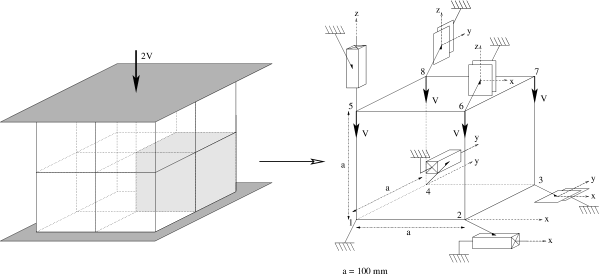
Figure 6: Patch test

More precisely, a confinement pressure is prescribed via a cohesion behaviour on the material [17] depending on a single coefficient $C_{0}$. A displacement is imposed on the upperside. Four models are compared to underline the pertinency of the two unilateral behaviour laws. Two of them are considered to obtain some limit behaviours ; the first one denoted Sand, is free of wire ; the second one denoted Reinforced sand, is a superposition of a sand model and an elastic “bilateral” model of the reinforcement. The “unilateral” TexSol model referred to §3.3 is denoted Texsol. A particular model is added denoted Spherical Texsol corresponding to the previous one with $\mu_{w}=0$.

• Elasticity : $E_{s}=200000\mbox{ MPa}$, $\nu_{s}=0.4$, $E_{w}=100000\mbox{ MPa}$, $\nu_{w}=0.3$

• Plasticity : $C_{0}=50\mbox{ MPa}$, $\theta_{f}=0.1$, $H_{k}=100\mbox{ MPa}$, $H_{i}=100\mbox{ MPa}$

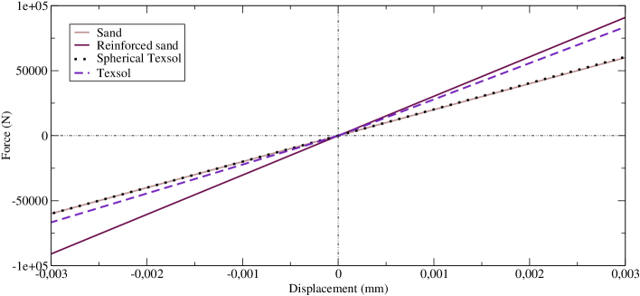
Figure 7: Zoom on the elastic range of the models

The Sand and the Reinforced sand appear clearly as two elastic bounds for TexSol models (cf. figure 7). At this stage, the Spherical Texsol does not differ from the Sand. On the contrary, the Texsol is close to the Sand in compression and close to the Reinforced sand in traction. For the two loadings the limit models reveal to be the upper bounds.

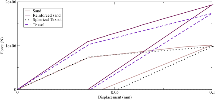
Figure 8: Different material behaviours on a traction patch test

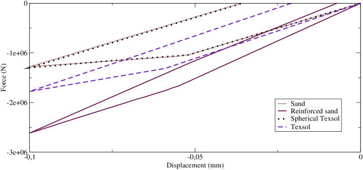
Figure 9: Different material behaviours on a compression patch test

For a loading-unloading traction process, the Texsol model behaves almost like the Reinforced sand as expected (cf. figure 8). The Spherical Texsol does not improve significantly the Sand (cf. figure 8 and 9). Consequently, the Spherical Texsol does not account for the numerical results given in the figure 3 for the same kind of experiment - even roughly.

4.3 Cyclic loading

TexSol embankments may be submitted to vibrating solicitations. A cyclic test based on the test represented in the figure 10 (where the displacements are fixed on the lower side and the sollicitation managed by force) is performed to underline the contribution of the “unilateral” reinforcement due to the wire network.

Figure 10: Force managed traction / compression test

Some material parameters are changed to apply a greater amplitude of loading on it : $C_{0}=150\mbox{ MPa}$, $\theta_{f}=0.02$, $H_{k}=5\mbox{ MPa}$, $H_{i}=1\mbox{ MPa}$. Reinforced sand, Texsol and Sand are compared in the figures 11, 12 and 13.

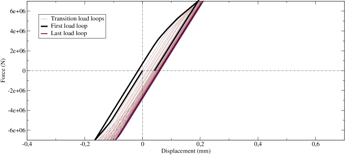
Figure 11: Reinforced sand behaviour on a cyclic test (20 loops)

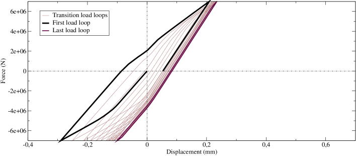
Figure 12: Texsol behaviour on a cyclic test (20 loops)

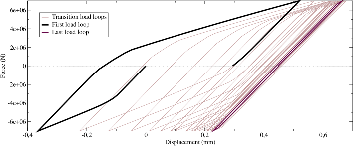
Figure 13: Sand behaviour on a cyclic test (20 loops)

For the three models, the response tends to be stabilized after 20 cycles. But for Reinforced sand and Texsol the stabilization is reached before 10 loops. Moreover the residual displacement of Texsol is $30$ percents bigger than that of Reinforced sand and five times smaller than that of Sand. This last result highlights the advantages of TexSol reinforcement. An other effect of the “unilateral” wire in the Texsol model is clearly illustrated by the curvature changes when the displacement switches sign in the figure 12.

4.4 Compression test

In soil mechanics it is usual to carry out a triaxial test with a prescribed confinement pressure (cf. fig 14). Considering the previous numerical results of the §4.2, the Spherical Texsol model is no more studied. Only the three other cases are compared in a loading compression test (the bulk mesh is described in [10]).

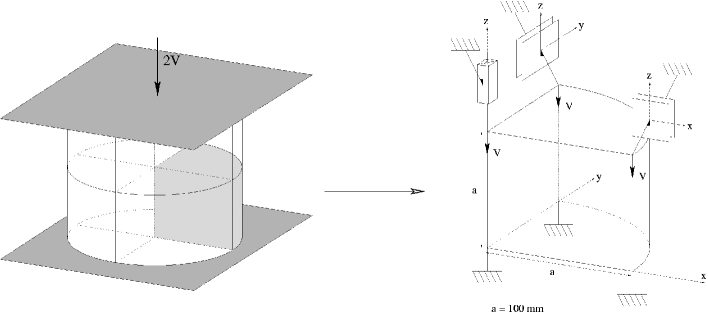
Figure 14: Compression test

The contribution of the wire in TexSol to the mechanical strenght is illustrated by the spacial distribution of two stresses : the full stress $\sigma$ and the wire stress $\mbox{\boldmath{$\sigma$}}_{w}$. The distribution of the full stress is identical in the three models with a level for Texsol between the two others.

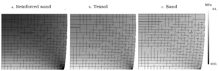
Figure 15: Equivalent Von-Mises stress

The main part of stress is located in the center of the bulk expect a localized concentration on the right lower corner. The contribution of the wire in the stress tensor ($\mbox{\boldmath{$\sigma$}}_{w}$) is split into its deviatoric part and its spherical one (pressure). Both parts are identically null for Sand (cf. figure 16c and 17c).

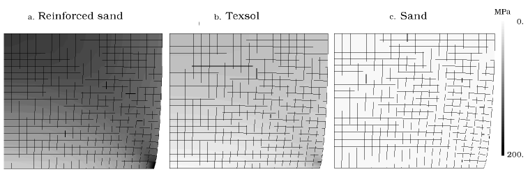
Figure 16: Wire equivalent Von-Mises stress

The elasticity of the reinforcement is activated only in tensile directions for the Texsol and in all directions for the Reinforced sand ; this explains the different full stress levels in the figure 15 and the different wire stress levels in the figure 16.

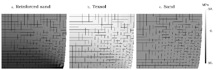
Figure 17: Wire pressure

The nature of the reinforcement due to the wire is clearly illustrated in the figure 17. The wire pressure in the Sand sample is of course identically null. It is negative in the Texsol wire (traction behaviour) according to the unilaterality condition expressed in the equation (20) whereas the pressure in the reinforcement of the Reinforced sand is almost everywhere positive.

5 Conclusion and prospects

In this paper a coherent thermodynamical model is proposed to account for numerical experiments (because of the lack of real experiments on the TexSol). The keypoint is a “unilateral” elasticity which model the wire network. An elastic plastic model is superposed to the previous one to obtain both strain formulation and stress formulation when it is possible. Using a finite element method, we roughly validate the expected behaviour.

The main perspective of this work is the identification of the mechanical parameters of the superposed model by series of numerical experiments in progress. In a more general framework orthotropic model is generally usefull to model the wire network.

The free energy $\psi$ considered in this work is postulated and in some cases we can write the free enthalpy via the Legendre–Fenchel transformation. Another approach should be to postulate the free enthalpy using a form similar to (19),

$$\mathscr{G}_{w}=\frac{\nu_{w}}{2E_{w}}\langle\mbox{tr}(\mbox{\boldmath{$\sigma$}}_{w})\rangle^{2}+\frac{1-\nu_{w}}{2E_{w}}\mbox{\boldmath{$\sigma$}}^{\geq}_{w}:\mbox{\boldmath{$\sigma$}}^{\geq}_{w}\mbox{ .}$$

The link between $\mathscr{G}_{w}$ and $\psi^{*}_{w}$ is an open question because in a three dimensional case the convexity of $\psi$ cannot be proved.

Acknowledgement

Thanks to Dr. Keryvin from the LARMAUR (Rennes) for his theoric and logistics supports.

References

• [1] D. CAMBOU, M. JEAN : Micromécanique des matériaux granulaires. Hermès. Science-Paris, 2001.
• [2] F.H. CLARKE : Optimization and nonsmooth analysis. Wiley-Interscience Philadelphia, 1983. Republished as F.H. Clarke, Classics in Applied Mathematics, vol. 5, SIAM, New-York, 1990.
• [3] F. DUBOIS, M. JEAN : LMGC90 une plateforme de développement dédiée à la modélisation des problèmes d’interaction. $\mbox{6}^{\mbox{th}}$ CNCS Giens, vol. 1, p. 111-118, 2003.
• [4] D. DRUCKER, W. PRAGER : Soil mechanics and plastic analysis of limit design. Quart. Appl. Math., vol. 10, p. 157-165, 1952.
• [5] M. FREMOND : Non-Smooth Thermo-mechanics. Springer-Verlag Berlin Heidelberg New York, 2002.
• [6] B. HALPHEN, QS. NGUYEN : Sur les matériaux standards généralisés. Journal de Mécanique, $\mbox{n}^{\circ}$ 14, p. 39-63, 1975.
• [7] V. KERYVIN : Contribution à la modélisation de l’endommagement localisé. PhD Thesis, Université de Poitier, LMPM/LMA, 1999.
• [8] M. KHAY, J-P. GIGAN : TEXSOL - Ouvrage de soutènement. LCPC, 1990.
• [9] J. KICHENIN, T. CHARRAS : CAST3M - Implantation d’une nouvelle loi d’évolution / loi de comportement mécanique. SEMT/LM2S, 2003.
• [10] R. LANIEL : Simulation des procédés d’indentation et de rayage par éléments finis et éléments distincts. DEA, Université de Rennes I & INSA, 2004.
• [11] R. LANIEL, O. MOURAILLE, S. PAGANO, F. DUBOIS, P. ALART : Numerical modelling of reinforced geomaterials by wires using the Non Smooth Contact Dynamics. $\mbox{4}^{\mbox{th}}$ CMIS Hannover, 2005.
• [12] E. LEFLAIVE, M. KHAY, J-C. BLIVET : Un nouveau matériaux : le TEXSOL. Travaux, $\mbox{n}^{\circ}$ 602, p. 1-3, septembre 1985.
• [13] J. LEMAITRE, J-L. CHABOCHE : Mechanics of solid materials. Cambridge, 1990.
• [14] J-J. MOREAU : Fonctionnelles convexes. Séminaire Equations aux dérivés partielle, Collège de France, 1966.
• [15] J-J. MOREAU : Numerical aspects of the sweeping process. Comput. Methods Appl. Mech. Engrg., $\mbox{n}^{\circ}$ 177, p. 329-349, 1999.
• [16] O. MOURAILLE : Etude sur le comportement d’un matériau longueur interne : le TexSol. DEA, Université de Montpellier II, 2004.
• [17] F. RADJAI, I. PREECHAWUTTIPONG, R. PEYROUX : Cohesive granular texture. [19], p. 149-162, 2001.
• [18] P. SUQUET : Plasticité et homogénéisation. PhD Thesis, Université Pierre et Marie Curie, 1982.
• [19] P-A. VERMEER, S. DIEBELS, W. EHLERS, H-J. HERMANN, S. LUDWIG, E. RAMM (Eds.) : Continuous and discontinuous modelling of cohesive frictionnal materials. Springer Berlin, 2001.
• [20] P. VILLARD : Etude du renforcement des sables par des fils continus. PhD Thesis, Université de Nantes, ENSM, 1988.
• [21] D.M. WOOD : Soil behaviour and critical state soil mechanics. Cambridge, 1990.