Photoionization of helium-like ions in asymptotic nonrelativistic region

Abstract

The cross section for single K-shell ionization by a high-energy photon is evaluated in the next-to-leading order of the nonrelativistic perturbation theory with respect to the electron-electron interaction. The screening corrections are of particular importance for light helium-like ions. Even in the case of neutral He atom, our analytical predictions turn out to be in good agreement with the numerical calculations performed with the use of the sophisticated wave functions. The universal high-energy behavior is studied for the ratio of double-to-single photoionization cross sections. We also discuss the fast convergence of the perturbation theory over the reversed nuclear charge number $1/Z$.

The single and double photoeffects on the helium isoelectronic sequence represent the simplest fundamental processes, which are being intensively investigated during last decades 1 ; 2 ; 3 ; 4 ; 5 ; 6 . The accurate treatment of electron correlations is still one of the main theoretical problems. Due to recent developments of novel synchrotron radiation sources, the study of the ionization of inner-shell electrons by high-energy photons is of particular interest.

For the theoretical description of the ionization processes on light atomic systems, it is usual to employ sophisticated methods with highly correlated wave functions. This allows one to take into account electron correlation effects beyond the independent-particle approximation. However, all the methods suffer from the gauge dependence. The latter can serve as a level of accuracy for the theoretical predictions. In addition, the final results for cross sections of the ionization processes are presented in a numerical form, which is not always easy to analyze.

In the case of heavy multicharged ions, on the contrary, the usual starting point is the approximation of non-interacting electrons, which are described by the Coulomb wave functions for the discrete and continuous spectra. The electron-electron interaction is treated within the framework of perturbation theory, which is also referred to as the expansion with respect to the parameter $1/Z$. The latter represents the ratio of the strength of the electron-electron interaction to the electron-nucleus one. To leading orders, perturbation theory allows one to derive analytical results. Accounting for higher-order correlation corrections improves the accuracy of the analytical predictions in the domain of lower values of the nuclear charge number $Z$. The results obtained within the framework of perturbation theory for the binding energies and for the cross sections are gauge independent.

In this Letter, we evaluate the next-to-leading-order correlation correction to the cross section for single K-shell ionization at asymptotic photon energies $\omega$ characterized by $I\ll\omega\ll m$, where $I=\eta^{2}/(2m)$ is the Coulomb potential for single ionization with $\eta=m\alpha Z$ being the average momentum of a K-shell electron, $m$ is the electron mass, and $\alpha$ is the fine-structure constant ($\hbar=1$, $c=1$). The ejected electrons are considered as being nonrelativistic. Accordingly, the Coulomb parameter is supposed to be sufficiently small, that is, $\alpha Z\ll 1$.

Neglecting terms of order $(\alpha Z)^{2}$, the operator describing the electron-photon interaction reads 7

$$\hat{V}_{\gamma}=N_{\gamma}e^{i(\bm{k}\cdot\bm{r})}\left(\bm{\mathrm{e}}\cdot\hat{\bm{p}}\right)\,,\qquad N_{\gamma}=\frac{1}{m}\frac{\sqrt{4\pi\alpha}}{\sqrt{2\omega}}\,.$$ (1)

Here $\hat{\bm{p}}$ is the momentum operator of an electron, which, in the coordinate representation, is cast into the gradient form $\hat{\bm{p}}=-i\bm{\nabla}$. An incoming photon is characterized by the momentum $\bm{k}$, the energy $\omega=|\bm{k}|=k$, and the polarization vector $\bm{\mathrm{e}}$. We employ the Coulomb gauge, in which $(\bm{\mathrm{e}}\cdot\bm{k})=0$ and $(\bm{\mathrm{e}}^{*}\cdot\bm{\mathrm{e}})=1$. In general, the nonrelativistic interaction between an electron and a photon includes also spin-dependent terms. However, in the case of single and double photoeffects the corresponding contributions to the cross sections are strongly suppressed 8 ; 9 ; 10 and, therefore, can be neglected.

In the nonrelativistic approximation, spatial and spin parts of two-electron wave functions factorize. Moreover, the operator (1) does not involve the spin matrices. As a result, the spin functions can be omitted throughout this consideration, while the symmetry of the coordinate wave functions $\Psi(\bm{r}_{1},\bm{r}_{2})$ is preserved in the ionization process. The total amplitude of the single photoeffect on helium-like ion is given by

$${\cal A}=2\,\langle\Psi_{f}|\hat{V}_{\gamma}|\Psi_{i}\rangle\,,$$ (2)

where the factor $2$ accounts for the one-particle character of the operator (1). That is, it is sufficient to consider the interaction of an incoming photon with a single atomic electron only.

In first-order perturbation theory with respect to the electron-electron interaction, the wave functions $\Psi_{i,f}$ of the initial and final states are represented as follows $\Psi_{i,f}\simeq\Psi^{(0)}_{i,f}+\Psi^{(1)}_{i,f}$. Accordingly, the amplitude of the process is just ${\cal A}\simeq{\cal A}^{(0)}+{\cal A}^{(1)}$. Neglecting the electron-electron interaction, we shall employ the single-particle approximation in the external Coulomb field of the nucleus (Furry picture):

$$\Psi_{i}^{(0)}(\bm{r}_{1},\bm{r}_{2}) = \psi_{1s}(\bm{r}_{1})\psi_{1s}(\bm{r}_{2})\,,$$ (3)

$$\Psi_{f}^{(0)}(\bm{r}_{1},\bm{r}_{2}) = \frac{1}{\sqrt{2}}\left[\psi_{\bm{p}}(\bm{r}_{1})\psi_{1s}(\bm{r}_{2})+\psi_{\bm{p}}(\bm{r}_{2})\psi_{1s}(\bm{r}_{1})\right]\,.$$ (4)

Here $\bm{p}$ is the momentum of escaping electron at infinity. The explicit expressions for the first-order corrections $\Psi^{(1)}_{i,f}$ to the wave functions can be found in works 10 ; 11 .

In zeroth approximation, the amplitude (2) looks as follows

$${\cal A}^{(0)}=2\,\langle\Psi_{f}^{(0)}|\hat{V}_{\gamma}|\Psi_{i}^{(0)}\rangle=\sqrt{2}\,\langle\psi_{\bm{p}}|\hat{V}_{\gamma}|\psi_{1s}\rangle\,.$$ (5)

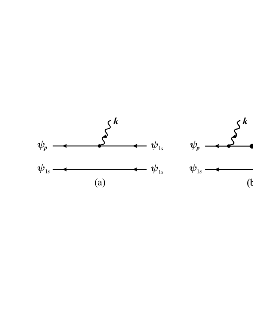
Figure 1: Feynman diagrams for the single ionization of K-shell electrons by a single photon. Solid lines denote electrons in the Coulomb field of the nucleus, the dashed line denotes the electron-electron Coulomb interaction, and the wavy line denotes an incident photon. The line with a heavy dot corresponds to the reduced Coulomb Green’s function. Diagram (a) does not account for the electron-electron interaction, while diagram (b) accounts for it in the initial state.

The matrix element (5) can be represented by the Feynman graph depicted in Fig. 1(a). Apart from the common factor, the expression (5) coincides with the amplitude for single photoeffect on hydrogen-like ion in the ground state.

In the asymptotic region, the energy and momentum conservation laws for the single K-shell photoionization keep the same form for both H- and He-like ions:

$$E_{p} = E_{1s}+\omega\simeq\omega\,,$$ (6)

$$\bm{p} = \bm{q}+\bm{k}\,.$$ (7)

Here $E_{1s}=-I$ is the Coulomb energy of the K-shell electron and $-\bm{q}$ is the recoil momentum transferred to the nucleus.

Let us evaluate the amplitude (5) using the momentum representation. Within the Born approximation, the wave function of the ejected high-energy electron is described by a plane wave, that is,

$$\langle\bm{f}|\psi_{\bm{p}}\rangle\simeq\langle\bm{f}|\bm{p}\rangle=(2\pi)^{3}\delta(\bm{f}-\bm{p})\,.$$ (8)

Here the standard normalization on $\delta$ function in the momenta is employed. Then the matrix element (5) yields

$${\cal A}^{(0)}=\sqrt{2}\,N_{\gamma}\langle\bm{q}|\psi_{1s}\rangle\left(\bm{\mathrm{e}}\cdot\bm{p}\right)\,.$$ (9)

If $q\gg\eta$ holds, the Coulomb wave function of the K-shell electron reads

$$\langle\bm{q}|\psi_{1s}\rangle\simeq N_{1s}\frac{8\pi\eta}{q^{4}}\,,$$ (10)

where $N^{2}_{1s}=\eta^{3}/\pi$. Since in the nonrelativistic domain the momentum $\bm{k}$ of a photon is negligibly small with respect to the electron momentum $\bm{p}$, relation (7) can be written as

$$\bm{p}\simeq\bm{q}\,.$$ (11)

The latter is equivalent to the use of the dipole approximation. Then one can set $q^{2}=p^{2}=2m\omega$ into Eq. (10). The amplitude (9) can be further simplified. The corresponding expression for the total cross section is well known 7

$$\sigma^{+}_{0}=\frac{2^{8}\pi\alpha}{3m\omega}\left(\frac{I}{\omega}\right)^{5/2}\,,\qquad(I\ll\omega\ll m)\,.$$ (12)

If the photon energy is not too high, as the wave function of the final state one needs to utilize the one-electron Coulomb wave function of the continuous spectrum. Accordingly, within the dipole approximation the amplitude (5) leads to the following expression for the total cross section,

$$\sigma^{+}_{\mathrm{C}}=\alpha a_{0}^{2}\,\frac{2^{10}\pi^{2}}{3Z^{2}}\frac{\exp(-4\xi\cot^{-1}\xi)}{\varepsilon^{4}_{\gamma}[1-\exp(-2\pi\xi)]}\,,\qquad(\omega\ll m)\,,$$ (13)

which is in fact valid in the whole nonrelativistic domain 7 . Here $\varepsilon_{\gamma}=\omega/I$ denotes the dimensionless energy for the incident photon, $a_{0}=1/(m\alpha)$ is the Bohr radius, and $\xi=1/\sqrt{\varepsilon_{\gamma}-1}$. The dimensionless parameter $\xi^{-1}=p/\eta$ has the meaning of the momentum $p$ of the ejected electron, which is calibrated in units of the characteristic momentum $\eta$. Formula (12) provides just the leading term in the expansion of Eq. (13) with respect to the parameter $\xi\ll 1$. Since the expression (13) involves the combination $\pi\xi$, the convergence of the $\xi$ expansion is slow. Note also that both cross sections (12) and (13) are twice as large as that for the single photoeffect on a hydrogen-like ion in the ground state. This is the consequence of the approximation of non-interacting electrons employed in the derivation. Neither $\sigma^{+}_{0}$ nor $\sigma^{+}_{\mathrm{C}}$ account for electron correlation effects.

Now we shall consider in more details the evaluation of the next-to-leading-order correction ${\cal A}^{(1)}$ to the amplitude of single K-shell photoeffect on helium-like ion. In the high-energy nonrelativistic limit, the dominant contribution to the amplitude of the process arises only from the Feynman diagram depicted in Fig. 1(b), providing the Coulomb gauge is employed. This graph accounts for the interaction between the electrons in the initial state. All other diagrams, namely, the one, which accounts for the electron-electron interaction in the final state, together with both exchange diagrams, turn out to be suppressed by the factor of about $I/\omega$ and, therefore, can be neglected. Accordingly, we can write

$${\mathcal{A}}^{(1)}=\sqrt{2}\,\langle\psi_{\bm{p}}\psi_{1s}|\hat{V}_{\gamma}G_{\mathrm{R}}(E_{1s})V_{12}|\psi_{1s}\psi_{1s}\rangle\,.$$ (14)

Here the operator $V_{12}$ describes the Coulomb electron-electron interaction. In the coordinate representation, it reads

$$V_{12}=\frac{\alpha}{|\bm{r}_{1}-\bm{r}_{2}|}\,.$$ (15)

The reduced Green’s function $G_{\mathrm{R}}(E_{1s})$ corresponding to the energy $E_{1s}$ of the K-shell electron is related to the usual nonrelativistic Coulomb Green’s function $G_{\mathrm{C}}(E)$ as follows

$$G_{\mathrm{R}}(E_{1s})=\lim_{E\to E_{1s}}\left\{G_{\mathrm{C}}(E)-\frac{|\psi_{1s}\rangle\langle\psi_{1s}|}{E-E_{1s}}\right\}\,.$$ (16)

Within the Born approximation (8), the amplitude (14) yields

$${\mathcal{A}}^{(1)} = 4\pi\alpha\sqrt{2}\,N_{\gamma}\left(\bm{\mathrm{e}}\cdot\bm{p}\right)\int\langle\bm{q}|G_{\mathrm{R}}(E_{1s})|\bm{f}_{1}\rangle\frac{1}{\bm{f}^{2}}\langle\bm{f}_{1}+\bm{f}|\psi_{1s}\rangle\times$$ (17)

$$\times\langle\psi_{1s}|\bm{f}_{2}\rangle\langle\bm{f}_{2}-\bm{f}|\psi_{1s}\rangle\frac{d\bm{f}_{1}}{(2\pi)^{3}}\frac{d\bm{f}_{2}}{(2\pi)^{3}}\frac{d\bm{f}}{(2\pi)^{3}}\,,$$

where $\bm{q}=\bm{p}-\bm{k}$. Integrating over the intermediate momenta in Eq. (17), one receives

$${\mathcal{A}}^{(1)} = 4\pi\alpha\sqrt{2}\,N_{\gamma}N_{1s}^{3}\left(\bm{\mathrm{e}}\cdot\bm{p}\right)\times$$ (18)

$$\times\left(-\frac{\partial}{\partial\mu}\right)\frac{1}{\mu^{2}}\langle\bm{q}|G_{\mathrm{R}}(E_{1s})\left(V_{i\eta}-V_{i(\eta+\mu)}\right)|0\rangle_{\left|\mu=2\eta\right.}\,,$$

$$\langle\bm{f}^{\prime}|V_{i\lambda}|\bm{f}\rangle = \frac{4\pi}{(\bm{f}^{\prime}-\bm{f})^{2}+\lambda^{2}}\,.$$

After taking the derivative with respect to $\mu$, one should set $\mu=2\eta$, where $\eta=m\alpha Z$.

In Eq. (18), we shall evaluate first the matrix element with the Coulomb Green’s function. Since $q\gg\eta$, one can employ the integral representation 12

$$\langle\bm{q}|G_{\mathrm{C}}(E)V_{i\lambda}|0\rangle \simeq 4m\eta\frac{ip_{1}}{q^{4}}\int_{1}^{\infty}\left(\frac{y+1}{y-1}\right)^{i\zeta}\langle 0|V_{p_{1}y+i\lambda}|0\rangle\,dy=$$ (19)

$$= 2^{5}\pi m\eta\frac{ip_{1}}{q^{4}}\int_{0}^{1}\frac{t^{-i\zeta}\,dt}{[\lambda(1-t)-ip_{1}(1+t)]^{2}}\,,$$ (20)

where $p_{1}=\sqrt{2mE}$ and $\zeta=\eta/p_{1}$. In order to isolate the pole contribution together with finite terms at $E\to E_{1s}$ in Eq. (20), we set $E=E_{1s}-\delta$. The shift $\delta$ is supposed to be small and positive. Expanding the intermediate momentum $p_{1}$ into a series over the parameter $\delta$, one receives

$$p_{1} \simeq i\eta(1+\varepsilon-\varepsilon^{2}/2)\,,$$ (21)

$$1-i\zeta \simeq \varepsilon(1-3\varepsilon/2)\,,$$ (22)

where $\varepsilon=\delta/(2I)$. Performing the integration in Eq. (20) by parts and using the expansions (21) and (22), we find that

$$\frac{ip_{1}}{\eta}\int_{0}^{1}\frac{t^{-i\zeta}\,dt}{[\lambda(1-t)-ip_{1}(1+t)]^{2}} \simeq -\frac{1}{(\lambda+\eta)^{2}}\left(\frac{1}{\varepsilon}+\frac{3}{2}+\frac{\lambda-\eta}{\lambda+\eta}\right)+$$ (24)

$$+2(\lambda-\eta)\int_{0}^{1}\frac{\ln t\,dt}{[\lambda+\eta-(\lambda-\eta)t]^{3}}\,.$$

In the integral (24) we have set $\delta=0$, which is equivalent to the substitution $ip_{1}\to-\eta$. As a result, the matrix element (19) can be cast into the form

$$\langle\bm{q}|G_{\mathrm{C}}(E_{1s}-\delta)V_{i\lambda}|0\rangle = 2^{5}\pi m\frac{\eta^{2}}{q^{4}}\left\{-\frac{1}{(\lambda+\eta)^{2}}\left(\frac{1}{\varepsilon}+\frac{3}{2}+\frac{\lambda-\eta}{\lambda+\eta}\right)+\right.$$ (25)

$$\left.+2(\lambda-\eta)\int_{0}^{1}\frac{\ln(1-t)\,dt}{[2\eta+(\lambda-\eta)t]^{3}}+\cal{O}(\varepsilon)\right\}\,.$$

The analogous matrix element involving the reduced Green’s function can be evaluated by making use of the definition (16):

$$\langle\bm{q}|G_{\mathrm{R}}(E_{1s})V_{i\lambda}|0\rangle=\lim_{\delta\to 0}\left\{\langle\bm{q}|G_{\mathrm{C}}(E_{1s}-\delta)V_{i\lambda}|0\rangle+\frac{1}{\delta}\langle\bm{q}|\psi_{1s}\rangle\langle\psi_{1s}|V_{i\lambda}|0\rangle\right\}\,.$$ (26)

The counter-term in Eq. (26) is given by

$$\frac{1}{\delta}\langle\bm{q}|\psi_{1s}\rangle\langle\psi_{1s}|V_{i\lambda}|0\rangle=\frac{2^{5}\pi m\eta^{2}}{\varepsilon q^{4}(\lambda+\eta)^{2}}\,.$$ (27)

Here the explicit expression for the matrix element

$$\langle\psi_{1s}|V_{i\lambda}|0\rangle=N_{1s}\frac{4\pi}{(\lambda+\eta)^{2}}$$ (28)

and Eq. (10) have been employed.

Adding Eqs. (25) and (27), one observes that the pole terms cancel each other. Accordingly, we arrive at the following expression

$$\langle\bm{q}|G_{\mathrm{R}}(E_{1s})V_{i\lambda}|0\rangle = -2^{5}\pi m\frac{\eta^{2}}{q^{4}}\left\{\frac{3}{2(\lambda+\eta)^{2}}+\right.$$ (29)

$$\left.+\frac{(\lambda-\eta)}{(\lambda+\eta)^{3}}-2(\lambda-\eta)\int_{0}^{1}\frac{\ln(1-t)\,dt}{[2\eta+(\lambda-\eta)t]^{3}}\right\}\,.$$

Using Eq. (29) allows one to evaluate analytically the matrix element entering Eq. (18). It yields

$$N_{1s}^{2}\left(-\frac{\partial}{\partial\mu}\right)\frac{1}{\mu^{2}}\langle\bm{q}|G_{\mathrm{R}}(E_{1s})\left(V_{i\eta}-V_{i(\eta+\mu)}\right)|0\rangle_{\left|\mu=2\eta\right.}=\frac{m}{q^{4}}a_{1}\,.$$ (30)

Here the coefficient $a_{1}$ appears as

$$a_{1}=-\frac{19}{16}+\frac{3}{4}\ln 2\simeq-0.6676\,.$$ (31)

The next-to-leading-order correction ${\cal A}^{(1)}$ to the amplitude of the single photoionization of helium-like ion in the ground state is given by

$${\mathcal{A}}^{(1)}=\sqrt{2}\,N_{1s}N_{\gamma}\frac{4\pi\eta}{Zq^{4}}\left(\bm{\mathrm{e}}\cdot\bm{p}\right)a_{1}\,.$$ (32)

Employing Eqs. (9) and (10) yields the total amplitude

$${\mathcal{A}}={\mathcal{A}}^{(0)}+{\mathcal{A}}^{(1)}={\mathcal{A}}^{(0)}\left(1+\frac{a_{1}}{2Z}\right)\,,$$ (33)

which accounts for the electron correlations. Within the same approximation, the total cross section for the single K-shell photoionization reads

$$\sigma^{+}=\sigma_{0}^{+}\left(1+a_{1}Z^{-1}\right)\,,$$ (34)

where $\sigma^{+}_{0}$ is given by Eq. (12).

The negative sign of the coefficient (31) can be understood on the qualitative ground. It is well known that the single photoeffect does not proceed on the free electron, while it can occur on the bound one 7 . The explanation of this fact follows from the relation (11): the nucleus serves as an absorber of the recoil momentum $\bm{q}$. In the asymptotic region, the value of $\bm{q}$ is relatively large, since the condition $q\gg\eta$ holds. The Coulomb calculation performed within the approximation of non-interacting electrons overestimates the cross section, because the electron-nucleus bindings are utmost strong in this case. Accounting for the screening effects attenuates these bindings, so that, the cross section of the single photoionization reduces in the absolute value.

As we already mentioned, if the photon energy is not too high, the cross section $\sigma^{+}_{\mathrm{C}}$ is more preferable rather than $\sigma^{+}_{0}$. Due to slow convergence of the expansion of Eq. (13) with respect to the parameter $\xi$, it is still legitimate to use of the following formula

$$\sigma^{+}=\sigma_{\mathrm{C}}^{+}\left(1+a_{1}Z^{-1}\right)$$ (35)

instead of Eq. (34).

As a testing ground for our analytical results, we choose the neutral He atom, which seems to be the most thoroughly investigated two-electron system. However, although extensive numerical calculations of the photoionization cross sections have been published in the literature, there are significant disagreements between predictions based on different sophisticated methods at high photon energies. The difficulty of comparison with experimental data arises due to presence of additional contributions from the scattering channels. One measures the total attenuation cross section, but not exclusively the photoionization one 1 ; 2 . As the most accurate theoretical calculations of the photoionization cross sections at high-energy domain, Samson et. al. 1 have selected results of the work 13 . Bell and Kingston used the Hartree-Fock wave function for the continuum state and many-parametrical variational wave function for the ground state. At $\omega\simeq 3.5$ keV their result for the cross section is equal to $5.74$ b, which however exhibits a gauge dependence on the level of about $6\%$ 13 . Our analytical formulas (34) and (35) yield $8.24$ b and $5.73$ b, respectively. In this case, the parameter $\xi=1/8$, but the value $\pi\xi$ is not too small.

In the double photoeffect, one is usually interested in the ratio of double-to-single ionization cross sections. At high photon energies, the calculations performed within the framework of the leading-order perturbation theory yield

$$R_{0}=\frac{\sigma^{++}_{0}}{\sigma^{+}_{0}}=\frac{B}{Z^{2}}\,,$$ (36)

where $B=0.090$ 14 ; 15 and $\sigma^{+}_{0}$ is given by Eq. (12). Taking into account the higher-order screening corrections to the total cross sections leads to the following expression for the universal asymptotic ratio

$$R=R_{0}\frac{(1+b_{1}Z^{-1}+b_{2}Z^{-2}+\ldots)}{(1+a_{1}Z^{-1}+a_{2}Z^{-2}+\ldots)}\,.$$ (37)

The factor $R_{0}$ is separated out here, since the electron binding energy is supposed to be negligibly small compared to the photon energy. To any given order of the perturbation theory with respect to the electron-electron interaction the representation (37) is the Padé approximant. The next-to-leading-order coefficient $a_{1}$ is given by Eq. (31), while the other coefficients remain to be calculated. Nevertheless, employing experimental data for the double-to-single photoionization ratio, one can deduce an estimate for the value of the coefficient $b_{1}$. The latter can be obtained by equating the experimental value $R^{\mathrm{exp}}=1.72(12)\%$ measured for He atom 3 and the theoretical ratio (37) truncated with taking into account only the next-to-leading-order correlation corrections. It yields

$$b_{1}=-0.981(71)\,.$$ (38)

Having fixed the coefficients $a_{1}$ and $b_{1}$, we have calculated the double-to-single photoionization ratio for helium isoelectronic sequence. In Table 1, we present a comparison of our next-to-leading-order predictions according to Eq. (37) with the numerical results obtained by Forrey et al. 4 . The account of the screening corrections improves significantly the asymptotic behavior for the leading-order ratio $R_{0}$ in the case of light two-electron systems. This supports the statement concerning the fast convergence of the $1/Z$ expansion even in the extreme nonrelativistic domain 16 . Indeed, the starting approximation of the perturbation theory (assuming non-interacting electrons) would be utmost inadequate for the description of light helium-like ions, which are highly correlated. The relatively large values for the coefficients (31) and (38) allow to correct the zeroth approximation. Note also that the double-to-single photoionization ratio (37) turns out to be less sensitive to the higher-order screening corrections rather than the total cross sections, since the coefficients $a_{1}$ and $b_{1}$ have the same sign. Unfortunately, the significant uncertainty of the coefficient (38) distorts the true behavior of the ratio $R$ in the case of H^- ion. The coefficients $a_{2}$, $b_{1}$, and $b_{2}$ should be calculated exactly within the framework of the consistent perturbation theory.

Nevertheless, it is worthwhile to trace out the nontrivial behavior of the series over the parameter $1/Z$ taking the binding energy for the ground state in H^- ion as an example. Without the electron-electron interaction the Coulomb binding energy is equal to $27.2116$ eV. The corrections due to one-, two-, and three-photon exchange diagrams are known to yield $-17.0079$ eV, $4.2921$ eV 17 ; 18 , and $-0.1723$ eV 18 , respectively. Then the total binding energy turns out to be equal to $14.324$ eV. This should be compared with the exact numerical result of $14.361$ eV, which has been obtained within the approximation of an infinitely heavy nucleus 19 . On the level of accuracy of about $10^{-2}$ eV one already needs to take into account the effect of nuclear recoil. As seen, the terms of the $1/Z$ expansion exhibit sign-changing oscillations and decrease fast in their absolute value. Although the formal parameter of the perturbation theory is equal to 1, the actual expansion turns out to converge by one order of magnitude due to hidden parameters of the theory.

Concluding, we have evaluated the single K-shell photoionization cross section with taking into account the next-to-leading-order correlation correction. This allows one to improve the accuracy of analytical predictions for light helium-like ions at high-energy domain. We have discussed the universal behavior of the double-to-single photoionization ratio as well as the fast convergence of the perturbation theory with respect the parameter $1/Z$.

Table 1: The asymptotic ratios of double-to-single photoionization cross sections (in $\%$) are tabulated for various nuclear charge numbers $Z$. The ratio $R_{0}$ is calculated using the leading-order perturbation theory 14 ; 15 . The ratio $R$ is calculated according to the truncated expression (37), taking into account the next-to-leading-order corrections with the coefficients (31) and (38). The numerical calculations by Forrey et. al. 4 have been performed with the use of the fully correlated variational wave functions.

$Z$	$1$		$2$		$3$		$4$		$5$		$6$		$7$		$8$		$9$		$10$
$R_{0}$, Eq. (36)	9	.00	2	.25	1	.00	0	.56	0	.36	0	.25	0	.18	0	.14	0	.11	0	.09
$R$, Eq. (37)	0	.50	1	.72	0	.865	0	.509	0	.334	0	.235	0	.175	0	.135	0	.107	0	.087
$R$, Ref. 4	1	.602	1	.644	0	.856	0	.508	0	.334	0	.236	0	.175	0	.135	0	.107	0	.087

References

- (1) J.A.R. Samson, Z.X. He, L. Yin, G.N. Haddad, J. Phys. B 27 (1994) 887.
- (2) J.H. McGuire, N. Berrah, R.J. Bartlett, J.A.R. Samson, J.A. Tanis, C.L. Cocke, A.S. Schlachter, J. Phys. B 28 (1995) 913.
- (3) L. Spielberger, O. Jagutzki, R. Dörner, J. Ullrich, U. Meyer, V. Mergel, M. Unverzagt, M. Damrau, T. Vogt, I. Ali, Kh. Khayyat, D. Bahr, H.G. Schmidt, R. Frahm, H. Schmidt-Böcking, Phys. Rev. Lett. 74 (1995) 4615.
- (4) R.C. Forrey, H.R. Sadeghpour, J.D. Baker, J.D. Morgan III, A. Dalgarno, Phys. Rev. A 51 (1995) 2112.
- (5) J.S. Briggs, V. Schmidt, J. Phys. B 33 (2000) R1.
- (6) J. Berakdar, H. Klar, Phys. Rep. 340 (2001) 473.
- (7) A.I. Akhiezer, V.B. Berestetskii, Quantum Electrodynamics, Wiley, New York, 1974.
- (8) H.A. Bethe, E.E. Salpeter, Quantum Mechanics of One- and Two-Electron Atoms, Plenum, New York, 1977.
- (9) J.W. Cooper, Phys. Rev. A 47 (1993) 1841.
- (10) A.I. Mikhailov, I.A. Mikhailov, A.N. Moskalev, A.V. Nefiodov, G. Plunien, G. Soff, Phys. Rev. A 69 (2004) 032703.
- (11) E.J. Kelsey, J. Sucher, Phys. Rev. A 11 (1975) 1829.
- (12) M.Ya. Amusia, A.I. Mikhailov, Zh. Eksp. Teor. Fiz. 111 (1997) 862 [JETP 84 (1997) 474].
- (13) K.L. Bell, A.E. Kingston, J. Phys. B 4 (1971) 1308.
- (14) M.Ya. Amusia, E.G. Drukarev, V.G. Gorshkov, M.P. Kazachkov, J. Phys. B 8 (1975) 1248.
- (15) A.I. Mikhailov, I.A. Mikhailov, Zh. Eksp. Teor. Fiz. 114 (1998) 1537 [JETP 87 (1998) 833].
- (16) A.I. Mikhailov, I.A. Mikhailov, A.V. Nefiodov, G. Plunien, G. Soff, Pis’ma Zh. Eksp. Teor. Fiz. 78 (2003) 141 [JETP Lett. 78 (2003) 110].
- (17) I. Lindgren, H. Persson, S. Salomonson, L. Labzowsky, Phys. Rev. A 51 (1995) 1167.
- (18) O.Y. Andreev, (private communication).
- (19) A.M. Frolov, Phys. Lett. A 345 (2005) 173.