Multifractal Model of Asset Returns versus real stock market dynamics

Abstract

There is more and more empirical evidence that multifractality constitutes another and perhaps the most significant financial stylized fact. A realistic model of the financial dynamics should therefore incorporate this effect. The most promising in this respect is the Multifractal Model of Asset Returns (MMAR) introduced by Mandelbrot et al. [1] in which multifractality is carried by time deformation. In our study we focus on the Lux extension to MMAR and empirical data from Warsaw Stock Exchange. We show that this model is able to reproduce relevant aspects of the real stock market dynamics.

1 Introduction

Empirical data collected from the stock market has extremely complicated structure. Apparently, it can seem to be white noise without correlations and with complete disorder, but, by investigating it deeper by means of sophisticated methods, one discovers important non-random features and an amazing hierarchy. Amongst these key properties (the so-called stylized facts) are the fat tails of p.d.f. of the logarithmic returns, the long range correlations in volatility, the leverage effect and some nontrivial fractal characteristics of data  [2, 3, 4, 5, 6, 7]. Especially the fractal aspects seem to be particularly important due to their ability to describe complex systems in a relatively simple way. Scaling properties, which are fundamental in the fractal formalism, manifest themselves as a linear plot of a given quantity on a log-log scale and the systems exhibiting such behaviour are called scale-free. As many real-world signals, the financial data cannot be described as a single fractal object but rather as a structure comprising a whole family of interwoven fractals forming a multifractal. Thus, description of this kind of data requires idetifying all of its fractal components. The multifractal formalism was originally proposed in ref. [8] where the singularity spectrum $f(\alpha)$ was introduced as a tool characterizing a multifractal. This formalism allowed researchers to discover multifractality in almost all fields of science and has gradually become a powerful method quantifying time series coming from biology, physics, economics, technical science and many others [9, 10, 11].

Having identified the fractal properties of data, the next natural step of the analysis is to simulate a process capable of reproducing these properties under control. As regards the financial world, the two following models have been proposed. The Mandelbrot’s Multifractal Model of Assets Returns (MMAR) [1, 12, 13] approximates evolution of the returns with a compound process involving multifractal time and a monofractal fractional Brownian motion. In contrast, the Multifractal Random Walk (MRW) [14, 15] can be viewed as a continuous interpolation of a discrete multifractal cascade. What is particularly important in this context is that multifractal features are not reproduced in such popular models like the family of ARCH processes.

In our paper we refer only to MMAR model and, more specifically, to one of its extensions that we shall call the Lux model [16]. Unlike the static original MMAR model, it incorporates an iterative mechanism that mimics effects of the generating cascade for each consecutive point without limiting the length of a signal. An advantage of this innovation, that looks attractive especially from the perspective of financial engineering, is its forecasting power [17]. We show flexibility of the Lux model while an analyzed process changes dynamics. Inspecting the evolution of the model’s parameters can help us interpreting the multifractal properties of empirical data.

2 Multifractal formalism

Let us denote the increments of a stationary process $X(t)$ by [1]

$$X(t,\Delta t)=X(t+\Delta t)-X(t).$$ (1)

Multifractality of this process can be defined by a non-uniform scaling of the q-order correlation function $X(t,\Delta t)$

$$E[X(t,\Delta t)^{q}]\sim\Delta t^{\tau(q)+1},$$ (2)

where $\tau(q)$ denotes the scaling exponent. If $\tau(q)$ nonlinearly depends on $q$ we say that $X(t,\Delta t)$ possesses a multifractal character. In a case of linear behaviour of $\tau(q)$ such a process is called monofractal. An example of the monofractal dynamics is fractional Brownian motion which has no correlation (its classic version) or is only linearly correlated. $\tau(q)$ can be related to the singularity spectrum $f(\alpha)$ by applying the Legendre transformation [18]

$$\bigg{\{}\begin{array}[]{l}q=df/d\alpha\\ \tau(q)=q\alpha-f(\alpha)\ .\end{array}$$ (3)

For the Brownian motion the singularity spectrum consists of a single point localized at $\alpha=H$ ($H$ is the so-called Hurst exponent) and $f(\alpha)=1$, indicating a strong linear correlation (positive one for $H>0.5$ and negative one for $H<0.5$) or no correlation ($H=0.5$). For a signal with a multifractal structure the $f(\alpha)$ shape resembles an inverted parabola. The strength of multifractality can be quantified in terms of the $f(\alpha)$ curve width

$$\Delta\alpha=\alpha_{max}-\alpha_{min}.$$ (4)

The bigger $\Delta\alpha$ the richer multifractal (we can also say the more “convoluted” fractals). Multifractality of a signal can be detected by using one of the modern methods like Multifractal Detrended Fluctuation Analysis (MFDFA) [19] or Wavelet Transform Modulus Maxima (WTMM) [18]. Here we restrict the analysis to MFDFA which in our opinion gives more reliable results [20].

3 Nonlinear dynamics of WIG20

Recent studies show that fluctuation distribution of a market index cannot be well approximated by a Gaussian [2]. Probability density function of the returns is characterized by the so-called fat tails which in most cases obey an inverse cubic power law if expressed as c.d.f. [21]. However, in the case of an emerging market we cannot a priori exclude a different behaviour. In the beginning of our study we first verify if the stock price fluctuations on the Warsaw Stock Exchange (WSE) obey the same law as larger developed markets. Calculations were carried out on high frequency data of the WSE blue chips WIG20 index sampled with 1 minute resolution over the period 1999-2004. All the overnight returns were removed as they are contaminated by some spurious artificial effects. The WIG20 fluctuations are shown in Figure 1.

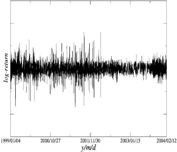
Figure 1: Time series of WIG20 log-returns covering the analyzed period.

What we can easily notice is that after the end of April 2002 the wildest fluctuations seem to be suppressed and the signal becomes “milder”. Thus, it is natural to divide our signal into the two following periods and consider them separately: the first one from January 1999 to April 2002 (237304 points) and the second one from May 2002 to December 2004 (237268 points). Cumulative distributions for both time series are presented in Figure 2.

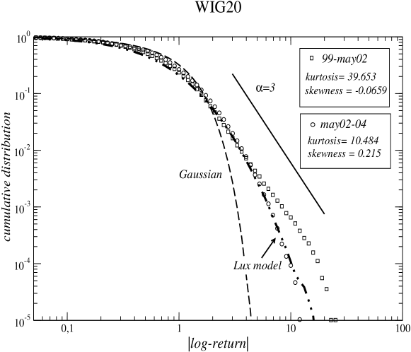
Figure 2: Cumulative distribution of WIG20 log-returns for periods 1999/01$-$2002/04 (squares) and 2002/05$-$2004/12 (circles) confronted against c.d.f.s of a Gaussian (dashed line) and of a signal generated according to Lux model (dash-dotted line).

In average they remain consistent with the inverse power cubic law. For the first period we actually have $\alpha=2.8$ but only for a very narrow range of plot, while for the second period a larger deviation is visible ($\alpha=4.2$). Consistently with the above conclusion from Figure 1, we see a difference in scaling properties between the periods. From a potential investor’s point of view, an even more important information is stored in temporal correlations of the analyzed signal. This information can be derived from its multifractal properties that can be a result of both the wide fluctuations distribution and the correlations in higher moments. It is instructive to calculate the $f(\alpha)$ spectra for each year individually and to identify changes in the signal evolution. The corresponding spectra are shown in Figure 3.

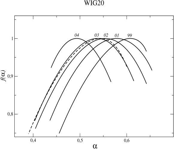
Figure 3: Singularity spectra of WIG20 log-returns splitted into annual intervals; two-digit numbers denote the corresponding year except for 2000 denoted by dashed line.

The most interesting feature of this Figure is that the $f(\alpha)$ maxima systematically shift towards lower $\alpha$’s: from $\alpha=0.61$ in 1999 to $\alpha=0.48$ in 2004), with the exception of 2000 (dashed line), suggesting a gradual transition from a strong persistence (1999) to a weak antipersistence (2004). Almost all the spectra are wide ($\Delta\alpha>0.2$) and can be interpreted as a manifestation of strong multifractality and rich dynamics. The narrowest curve is for 2004 ($\Delta\alpha=0.11$) so we can regard it as the least interesting one from the multifractal point of view.

4 Multifractactal Model of Asset Returns

According to MMAR the logarithmic price $P(t)$ is assumed to follow a compound process consisting of a fractional Brownian motion $B_{H}(t)$ and a time $\theta(t)$:

$$P(t)=B_{H}(\theta(t)).$$ (5)

Here $B_{H}$ represents a monofractal process which is a sum of random variables sampled by c.d.f. of a multifractal measure. Both $B_{H}$ and $\theta(t)$ are independent. A crucial role in the considered process plays the virtual trading time which can be interpreted as a deformation of the homogeneous clock-time or as a local volatility corresponding to faster or slower trading. The linear correlation of $P(t)$ depends on the Hurst exponent $H$ fully characterizing the Brownian motion, whereas the multifractal properties are generated by a multiplicative cascade. It has to be noted that in the original formalism of ref. [1] the whole cascade is generated globally at the same moment for each level $k$. However, for the sake of prediction we need an iterative procedure that is able to differentiate past and future events. This is the rationale behind the application of a multiplicative measure proposed by Lux [16].

Instead of $\theta$ it is better to consider its increments $\theta^{\prime}(t)$ expressed by [3]

$$\theta^{\prime}(t)=2^{k}\prod_{i=1}^{k}m_{i}(t),$$ (6)

where $2^{k}$ is a normalizing factor and $m_{i}$ is a random multiplier taken from the log-normal distribution in accordance with the formula

$$m_{t+1}^{i}=\bigg{\{}\begin{array}[]{l}\exp(N(-\lambda\ln 2,2(\lambda-1)\ln 2))\\ m_{t}^{(i)},\end{array}$$ (7)

where $i=1,...,k$ and $N(\mu,\sigma^{2})$ denotes the conventional normal distribution. The upper option is taken either with the probability $2^{-(k-i)}$ or if for any preceding $i$ this option has already been chosen. Otherwise the multiplier remains the same as for previous $t$. We can imitate in this way the structure of a binary cascade and, on average, preserve its essential features. Based on this construction we see that in order to describe the multifractal properties of such a cascade we need only one parameter $\lambda$. Theoretical multifractal spectrum is then given by

$$f(\alpha)=1-\frac{(\alpha-\lambda)^{2}}{4(\lambda-1)}.$$ (8)

This formula implies that $f(\alpha)$ is symmetric and has a maximum localized at $\alpha=\lambda$. Under the above formalism a return can be viewed as a composition of local volatility and white noise [16]

$$x(t)=\sqrt{\theta^{\prime}(t)}\sigma N(0,1)=\sqrt{2^{k}\prod_{i}^{k}m_{i}(t)}\sigma N(0,1).$$ (9)

5 WIG20 modelling

We try to mimic evolution of WIG20 based on the Lux extension to MMAR and observe how the changes in WIG20 dynamics influence the parameter $\lambda$ of the model. This gives us information about the model flexibility and its ability to simulate a highly nonstationary process like the WIG20 returns. Since fitting the model with a log-normal multiplier distribution requires to estimate only the parameter $\lambda$ defining the distribution of Eq. (7), it can be derived by using the relation [12]

$$f_{P}(\alpha)=f_{\theta}(\alpha/H)$$ (10)

and Eq. (8). First we consider the simplest case of $H=0.5$. The singularity spectrum can be estimated by means of MFDFA with polynomial order 2 [7]. Figure 2 shows c.d.f. of a time series generated according to the Lux model (dash-dotted line). This distribution has a somewhat thinner tail than the inverse cubic power law, but it is similar to c.d.f. for WIG20 from the period 2002/05$-$2004/12. In this case the model appropriately reconstructs the dynamics including large fluctuations.

The evolution of $\lambda$ is analyzed by using a moving window of length 20000 data points shifted by 2000 points. Such a window ensures that we obtain statistically reliable results. From Figure 4 we see that $\lambda$ strongly fluctuates over the analyzed period. Nevertheless, starting from the end of 2001 it forms a clearly decreasing trend.

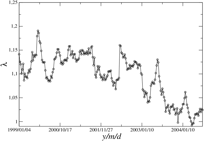
Figure 4: $\lambda$ calculated in a moving window as a function of time. Open symbols denote position of the first point for each window position.

The smallest values of $\lambda$ correspond to 2004 and even drop below 1. In the multifractal formalism $\lambda$ refers to the structure complexity; the larger $\lambda$ the more complicated signal and more complex fractal. It stems from this that from 2002 to 2004 the complexity of the Polish stock market gradually decreased despite the existence of some bigger fluctuations. This result remains in a perfect agreement with the indications of the $f(\alpha)$ spectra (Figure 3).

Although fixing $H$ value at 0.5 can give approximate results for shorter signals (e.g. of length of the window applied before), in general it is recommended to treat $H$ as a free parameter which has to be estimated from the data because it may influence the forecasted volatility [22]. To accomplish this task we have to use the relation between $f(\alpha)$ spectra for the price and the time processes (Eq. (10)) together with the following condition [13]:

$$\tau_{P}(1/H)=0.$$ (11)

where $\tau_{P}$ stands for the scaling exponent of the price process. The so-estimated Hurst exponent $H$ can be used in the calculation of $\lambda$. Results for the windowed WIG20 are collected in Figure 5.

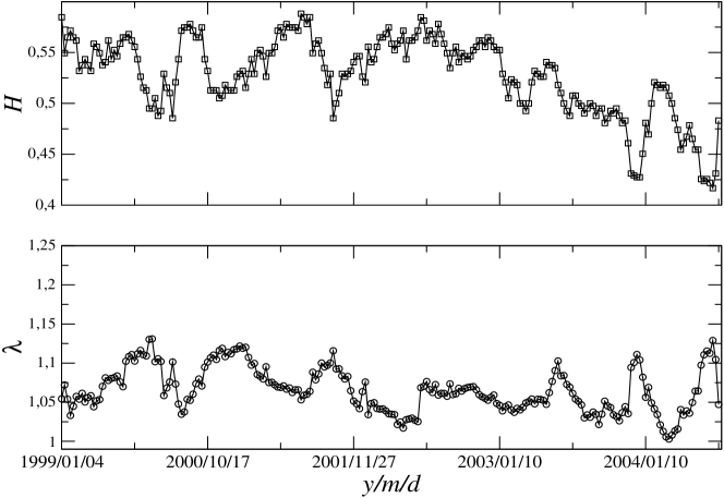
Figure 5: Simultaneous temporal evolution of Hurst exponent $H$ (top) and parameter $\lambda$ (bottom). Open symbols denote position of the first point for each window position.

For the first three-year-long interval the Hurst exponent indicate persistent behaviour of the index, while starting from 2002 the value of $H$ almost monotonically decreases below 0.5 suggesting a transition to the antipersistent regime. Again, this resembles the conclusion made from Figure 3 but now the evidence is even more convincing. As regards $\lambda$, we see that now its fluctuations are smaller and there is no clear decreasing trend. Therefore, in the present case of variable $H$ this quantity absorbs the information about changes in WIG20 dynamics.

6 Conclusions

The study presented in this paper reveals several interesting facts about dynamics of the Polish stock market. First, we see that the WIG20 fluctuation magnitude changes in the first half of year 2002. This suppression of the largest fluctuations is also visible in c.d.f. of the log-returns. Moreover, we identify this nonstationarity of WIG20 in evolution of the parameter $\lambda$ of the Lux model. These observations indicates that this model is able to reproduce at least some of the financial data characteristics and to help one with detecting evolution phases with different properties. In the last step we include in our analysis the empirical estimation of the Hurst exponent, a parameter which is necessary for the forecasting purpose. As our results document, value of this parameter largely determines the multifractal properties of the WIG20 evolution, leaving $\lambda$ only as an auxilliary measure.

References

- [1] B.B. Mandelbrot, L. Calvet, & A. Fisher, Cowles Foundation Discussion Papers: 1164 (1997).
- [2] P. Gopikrishnan, V. Plerou, L.A.N. Amaral, M. Meyer and H.E. Stanley, Phys. Rev. E 60, 5305-5316 (1999).
- [3] Z. Eisler, J. Kertész, Physica A 343, 603-622 (2004).
- [4] K. Matia, Y. Ashkenazy and H.E. Stanley, Europhys. Lett., 61 (3), pp. 422-428 (2003).
- [5] S. Drożdż, J. Kwapień, F. Grümmer, F. Ruf and J. Speth, Acta Physica Polonica B 34, 4293 (2003).
- [6] J. Kwapień, P. Oświȩcimka, S. Drożdż, Physica A 350, 466-474 (2005).
- [7] P. Oświȩcimka, J. Kwapień, S. Drożdż, Physica A 347, 626-638, (2005).
- [8] T.C. Halsey, M.H. Jensen, L.P. Kadanoff, I. Procaccia and B.I. Shraiman, Phys. Rev. A 33, 1141-1151 (1986)
- [9] P.Ch. Ivanov, L.A.N. Amaral, A.L. Goldgerger, S. Havlin, M.G. Rosenblum, Z. Sruzik, H.E. Stanley, Nature 399 461-465 (1999).
- [10] H.E. Stanley, L.A.N. Amaral, A.L. Goldberger, S. Havlin, P.Ch. Ivanov, C.-K. Peng, Physica A 270 309-324 (1999).
- [11] A. Bunde, Shlomo Havlin, Fractals and disordered systems, Springer-Velang (1991).
- [12] L. Calvet, A. Fisher, B.B. Mandelbrot, Cowles Foundation Discussion Paper 1165, (1997).
- [13] A. Fisher, L. Calvet and B.B. Mandelbrot (1997), Cowles Foundation Discussion Paper No. 1166, Yale University.
- [14] E. Bacry, J. Delour, J.F. Muzy, Phys. Rev. E 64, 026103 (2001)
- [15] J.F. Muzy, J. Delour,E. Bacry, Eur. Phys. J. B 17, 537-548 (2000).
- [16] T. Lux, The multi-fractal model of Asset Returns: its estimation via GMM and its use for volatility forecasting, University of Kiel, Working Paper, (2003).
- [17] T. Lux and Taisei Kaizoji, Forecasting volatility and volume in the Tokyo Stock Market: The Advantage of long memory models, University of Kiel, Working Paper, (2004).
- [18] J.F. Muzy, E. Bacry and Arneodo, National Journal of Bifurcation and Chaos, Vol. 2. No. 2 (1994) 245-302.
- [19] J.W. Kantelhardt, S.A. Zschiegner, E. Koscielny-Bunde, S. Havlin, A. Bunde, H.E. Stanley, Physica A 316, 87-114 (2002).
- [20] P. Oświȩcimka, J. Kwapień, S. Drożdż, Phys. Rev. E, in print (2006)
- [21] X. Gabaix, P. Gopikrishnan, V. Plerou, H.E. Stanley, Nature 423, 267-270 (2003)
- [22] A. Carbone, G. Castelli, H.E. Stanley, Physica A 344, 267-271 (2004).