Breakdown of Burton-Prim-Slichter approach and lateral solute segregation in radially converging flows

Abstract

A theoretical study is presented of the effect of a radially converging melt flow, which is directed away from the solidification front, on the radial solute segregation in simple solidification models. We show that the classical Burton-Prim-Slichter (BPS) solution describing the effect of a diverging flow on the solute incorporation into the solidifying material breaks down for the flows converging along the solidification front. The breakdown is caused by a divergence of the integral defining the effective boundary layer thickness which is the basic concept of the BPS theory. Although such a divergence can formally be avoided by restricting the axial extension of the melt to a layer of finite height, radially uniform solute distributions are possible only for weak melt flows with an axial velocity away from the solidification front comparable to the growth rate. There is a critical melt velocity for each growth rate at which the solution passes through a singularity and becomes physically inconsistent for stronger melt flows. To resolve these inconsistencies we consider a solidification front presented by a disk of finite radius $R_{0}$ subject to a strong converging melt flow and obtain an analytic solution showing that the radial solute concentration depends on the radius $r$ as $\sim\ln^{1/3}(R_{0}/r)$ and $\sim\ln(R_{0}/r)$ close to the rim and at large distances from it. The logarithmic increase of concentration is limited in the vicinity of the symmetry axis by the diffusion becoming effective at a distance comparable to the characteristic thickness of the solute boundary layer. The converging flow causes a solute pile-up forming a logarithmic concentration peak at the symmetry axis which might be an undesirable feature for crystal growth processes.

,

1 Introduction

Solidification and crystallisation processes are present in various natural phenomena as well as in a large number of material production technologies such as, for example, semiconductor crystal growth from the melt, alloy metallurgy, etc. Usually the melt used for the production of solid material is not a pure substance but rather a solution containing some dissolved dopants or impurities. Often the solid material grown from the solution has a non-uniform distribution of the dissolved substance although the original solution was uniform. This non-uniformity is caused by the difference of equilibrium concentrations of solute in the liquid and solid phases. Thus, if the equilibrium concentration of solute in a crystal is lower than in the melt, only a fraction of solute is incorporated from the melt into the growing crystal while the remaining part is repelled by the solidification front as it advances into the liquid phase [1]. This effect causes axial segregation of the solute, usually concentrated in a thin, diffusion-controlled boundary layer adjacent to the solidification front. Axial segregation can strongly be influenced by the melt convection. According to the original work by Burton, Prim and Slichter (BPS) [2], a sufficiently strong convection towards the crystallisation front reduces the thickness of the segregation boundary layer and so the solute concentration getting into the crystal. Such a concept of solute boundary layer has been widely accepted to interpret the effect of melt flow on the solute distribution in various crystal growth configurations [3, 4, 5]. The BPS approach, originally devised for a rotating-disk flow modelling an idealised Czochralski growth configuration, supposes the melt to be driven towards the solidification front by a radially diverging flow. However, in many cases, as for instance in a flow rotating over a disk at rest [6], like in a flow driven by a rotating [7] or a travelling [8] magnetic field, as well as in the natural convection above a concave solidification front in the vertical Bridgman growth process [9], the melt is driven away from the solidification front in its central part by a radially converging flow. Though several extensions of the BPS solution exist (e.g. [10, 11, 12, 13]), the possibility of a reversed flow direction away from the crystallisation front has not yet been considered in that context.

In this work, we show that the BPS approach becomes invalid for converging flows because the effective boundary layer thickness, which is the basic concept of the BPS theory, is defined by an integral diverging for a flow away from the solidification front. The divergence can formally be avoided by restricting the space occupied by the melt above the solidification front to a layer of finite depth, but for higher melt velocities this solution becomes physically inconsistent, too. Next we consider a solidification front as a disk of finite radius immersed in the melt with a strong converging flow and show that a converging flow results in a logarithmic solute segregation along the solidification front with a peak at the symmetry axis. An analytical solution is obtained by an original technique using a Laplace transform. The advantage of this solution is its simple analytical form as well as the high accuracy which has been verified by comparing with numerical solutions.

The simulation of dopant transport is an important aspect of crystal growth modelling [14, 15], and various numerical approaches are used for it. However, a numerical approach is always limited in the sense that it provides only particular solutions while the basic relations may remain hidden. Besides, the numerical solution often requires considerable computer resources when a high spatial resolution is necessary which is particularly the case for thin solute boundary layers. It has been shown, e.g., by Vartak and Derby [16] that an insufficient resolution of the solute boundary layer may lead to numerically converged but nevertheless inaccurate results.

The paper is organised as follows. In Section 2 we discuss the BPS-type approach and show its inapplicability to converging flows. The simple model problem of radial segregation along a disk of finite radius in a strong converging flow is described in Section 3, and an analytical solution for the concentration distribution on the disk surface is obtained in Section 4. Summary and conclusions are presented in Section 5.

2 Breakdown of BPS-type solutions

Consider a simple solidification model consisting of a flat radially-unbounded solidification front advancing at velocity $v_{0}$ into a half-space occupied by the melt which is a dilute solution characterised by the solute concentration $C.$ The latter is assumed to be uniform and equal to $C_{\infty}$ sufficiently far away from the solidification front. Solute is transported in the melt by both diffusion with a coefficient $D$ and the melt convection with a velocity field ${\boldsymbol{v}}$. At the solidification front, supposed to be at the thermodynamic equilibrium, the ratio of solute concentrations in the solid and liquid phases is given by the equilibrium partition coefficient $k$. In the absence of convection, the repelled solute concentrates in a boundary layer with the characteristic thickness $\delta_{0}=D/v_{0}$. We consider in the following the usual case of a much larger momentum boundary layer compared to the solute boundary layer, i.e. a high Schmidt number $\mathit{Sc}=\nu/D\gg 1$ where $\nu$ is the kinematic viscosity of the melt. The basic assumption of the BPS approach is that the lateral segregation is negligible and thus the solute transport is affected only by the normal velocity component. The latter is approximated in the solute boundary layer by a power series expansion in the distance $z$ from the solidification front as $v(z)\approx\frac{1}{2}v^{\prime\prime}(0)z^{2}.$ Then the equation governing the concentration distribution in the solute boundary layer may be written in dimensionless form as

$$-(1+\mathit{Pe}z^{2})\frac{dC}{dz}=\frac{d^{2}C}{dz^{2}},$$ (1)

where $\mathit{Pe}=\frac{v^{\prime\prime}(0)\delta_{0}^{3}}{2D}$ is the local Péclet number based on the characteristic boundary layer thickness $\delta_{0}$ which is used as length scale here while the concentration is scaled by $C_{\infty}.$ The boundary conditions for the uniformly mixed melt core and the solid-liquid interface take the form $\left.C\right|_{z\rightarrow\infty}\rightarrow 1$ and

$$\left[(1-k)C+\frac{dC}{dz}\right]_{z=0}=0.$$ (2)

The solution of this problem is

$$C(z)=1+A\int_{z}^{\infty}\exp\left(-t-\frac{\mathit{Pe}}{3}t^{3}\right)\,dt,$$ (3)

where the constant $A=\frac{1-k}{1-(1-k)\Delta(\mathit{Pe})}$ is obtained from (2) in terms of $\Delta(\mathit{Pe})=\int_{0}^{\infty}\exp\left(-t-\frac{\mathit{Pe}}{3}t^{3}\right)\,dt$ which according to the relation $C^{\prime}(0)=\frac{C(\infty)-C(0)}{\Delta(\mathit{Pe})}$ represents an effective dimensionless thickness of the solute boundary layer. Eventually, the concentration at the solidification front is obtained as $C(0)=\left[1-(1-k)\Delta(\mathit{Pe})\right]^{-1}$. This is the central result of the BPS approach stating that only the effective thickness of the solute boundary layer defined by the local velocity profile is necessary to find the solute concentration at the solidification front for a given uniform concentration in the bulk of the melt. However, it is important to note that this solution is limited to $\mathit{Pe}\geq 0$ and it becomes invalid for $\mathit{Pe}<0$ when the flow is directed away from the solidification front because both integrals in Eq. (3) and $\Delta(\mathit{Pe})$ diverge in this case. The goal of this study is to find out what happens to the solute distribution when the flow is directed away from the solidification front and the BPS solution breaks down.

Figure 1: Sketch of a radially unbounded flat layer with solidification and melting fronts at bottom and top, respectively.

The divergence in the BPS model for $\mathit{Pe}<0$ is obviously related to the unbounded interval of integration which can be avoided by taking into account the finite axial size of the system. The simplest such model, shown in Fig. 1, is provided by a flat, radially-unbounded layer between two disks separated by a distance $2H$. The upper and lower disks represent the melting and solidification fronts, respectively, and the molten zone proceeds upwards with velocity $v_{0}.$ There is a forced convection in the melt with the axial velocity $v(z)$ which is assumed to satisfy impermeability and no-slip boundary conditions. There is also a radial velocity component following from the incompressibility constraint which, however, is not relevant as long as a radially uniform concentration distribution is considered. Here we choose $H$ as a length scale so that the boundaries are at $z=\pm 1$. At the upper boundary, there is a constant solute flux due to the melting of the feed rod with the given uniform concentration $C_{0}$ with velocity $v_{0}$

$$\left.\mathit{Pe}_{0}(C-C_{0})+\frac{dC}{dz}\right|_{z=1}=0.$$

Note that this boundary condition following from the mass conservation does not formally satisfy the local thermodynamic equilibrium relating the solute concentrations in the solid and liquid phases. In order to ensure equilibrium concentrations at the melting front it would be necessary to take into account also the diffusion in the solid phase which, however, is neglected here. Such an approximation is justified by the smallness of the corresponding diffusion coefficient.

Figure 2: Modified effective boundary layer thickness $\mathit{Pe}_{0}\Delta(\mathit{Pe}_{0},\mathit{Pe}_{1})-1$ at the solidification front for a horizontal liquid layer of finite height with the flow away from the solidification front versus the Péclet number $\mathit{Pe}_{1}$ of melt stirring at various Péclet numbers $\mathit{Pe}_{0}$ based on the solidification rate.

At the lower boundary, coinciding with the moving solidification front, the boundary condition is

$$\left.(1-k)\mathit{Pe}_{0}C+\frac{dC}{dz}\right|_{z=-1}=0,$$ (4)

where $\mathit{Pe}_{0}=v_{0}H/D$ is the Péclet number based on the solidification velocity. The radially uniform concentration distribution depending only on the axial coordinate $z$ is governed by

$$\left(-\mathit{Pe}_{0}+\mathit{Pe}_{1}v(z)\right)\frac{dC}{dz}=\frac{d^{2}C}{dz^{2}},$$ (5)

where $\mathit{Pe}_{1}$ is the Péclet number of convection. The solution of the above equation is

$$C(z)=A+B\int_{-1}^{z}\exp\left[-\mathit{Pe}_{0}(t+1)+\mathit{Pe}_{1}\int_{-1}^{t}v(\tau)\,d\tau\right]\,dt.$$ (6)

The boundary condition (4) yields $B=-A(1-k)\mathit{Pe}_{0}$ while the remaining unknown constant $A$ is determined from the condition at the upper boundary. However, for our purposes it is sufficient to express $A$ in terms of the concentration at the solidification front: $A=C(-1).$ Then Eq. (6) allows us to relate the concentrations at the melting and solidification fronts

$$C(-1)=C(1)\left[1-(1-k)\mathit{Pe}_{0}\Delta(\mathit{Pe}_{0},\mathit{Pe}_{1})\right]^{-1},$$ (7)

where

$$\Delta(\mathit{Pe}_{0},\mathit{Pe}_{1})=\int_{-1}^{1}\exp\left[-\mathit{Pe}_{0}(t+1)+\mathit{Pe}_{1}\int_{-1}^{t}v(\tau)\,d\tau\right]\,dt$$ (8)

is the effective solute boundary layer thickness defined by the relation $\left.\frac{dC}{dz}\right|_{z=-1}=\frac{C(1)-C(-1)}{\Delta(\mathit{Pe}_{0},\mathit{Pe}_{1})}$ following from Eqs. (4) and (7). This effective boundary layer thickness at the solidification front is plotted in Fig. 2 for a model velocity distribution $v(z)=\left(1-z^{2}\right)^{2}$. The effective boundary layer thickness increases with the convection but the increase is relatively weak until $\mathit{Pe}_{1}$ becomes comparable to $\mathit{Pe}_{0}$. At this point, the effective thickness starts to grow nearly exponentially.

Although the effective boundary layer thickness is now bounded for any finite value of $\mathit{Pe}_{1}$ regardless of its sign defining the flow direction, the obtained solution is not really free from singularities. At first, note that the concentration at the solid-liquid interface becomes singular when the solute boundary layer becomes as thick as $\mathit{Pe}_{0}\Delta(\mathit{Pe}_{0},\mathit{Pe}_{1})=(1-k)^{-1}$ resulting in a zero denominator in Eq. (7). Second, for larger $\mathit{Pe}_{1}$ the denominator in Eq. (7) becomes negative implying a negative concentration at the solidification front that presents an obvious physical inconsistency. Thus, the obtained solution is applicable only for sufficiently weak converging flows and breaks down as the velocity of the melt flow away from the solidification front becomes comparable to the growth rate at $\mathit{Pe}_{1}\sim\mathit{Pe}_{0}.$

3 A disk of finite radius with a strong converging flow

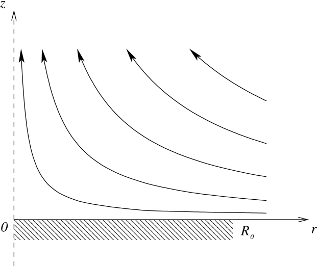
Figure 3: Sketch of the solidification front presented by a disk of radius $R_{0}$ in a converging flow.

The assumption underlying both the classical BPS approach and that of the previous section is the neglected radial segregation. The simplest physical model which could account for radial segregation is presented by a solidification front in the form of a disk of finite radius $R_{0}$ with the melt occupying the half-space above it, as shown in Fig. 3. For simplicity, the velocity distribution in the melt is assumed to be that of a liquid rotating above a disk at rest. In this case, contrary to the classical BPS problem of a rotating disk, the flow is radially converging rather than diverging. Thus, within the solute boundary layer, assumed as usual to be thin relative to the momentum boundary layer, the radial and axial velocity components can be approximated as

$$v_{r}\approx-\frac{1}{2}v_{z}^{\prime\prime}(0)rz,\qquad v_{z}\approx\frac{1}{2}v_{z}^{\prime\prime}(0)z^{2}.$$

Here we choose the thickness of the solute boundary layer based on the axial melt velocity as length scale

$$d_{0}=(2D/v_{z}^{\prime\prime}(0))^{1/3},$$ (9)

and assume the stirring of the melt to be so strong that the advancement of the solidification front with the growth velocity $v_{0}$ is small compared the characteristic melt flow in the solute boundary layer. The last assumption implies that the local Péclet number based on the growth rate is small: $\tilde{\mathit{Pe}}_{0}=v_{0}d_{0}/D\ll 1.$ Then the problem is defined by a single dimensionless parameter, the dimensionless radius $R=R_{0}/d_{0}=R_{0}(2D/v_{z}^{\prime\prime}(0))^{-1/3},$ which may be regarded as Péclet number based on the external length scale $R_{0}$ and the internal velocity scale $v_{0}=v_{z}^{\prime\prime}(0)d_{0}^{2}/2.$ The governing dimensionless equation is

$$z\left(z\frac{\partial C}{\partial z}-r\frac{\partial C}{\partial r}\right)=\frac{1}{r}\frac{\partial}{\partial r}\left(r\frac{\partial C}{\partial r}\right)+\frac{\partial^{2}C}{\partial z^{2}},$$ (10)

where the radial diffusion term will be neglected as usual for the boundary layer solution to be obtained in the following. Sufficiently far away from the solidification front a well-mixed melt is assumed with a uniform dimensionless concentration $C_{0}=1.$ The boundary condition at the solidification front

$$\left.\tilde{\mathit{Pe}}_{0}(1-k)C+\frac{\partial C}{\partial z}\right|_{z=0}=0,$$

for $\tilde{\mathit{Pe}}_{0}\ll 1$ suggests to search for the concentration as

$$C\approx C_{0}+\tilde{\mathit{Pe}}_{0}(1-k)C_{1},$$ (11)

where $C_{1}$ is the deviation of the concentration with a characteristic magnitude $\tilde{\mathit{Pe}}_{0}(1-k)\ll 1$ from its uniform core value $C_{0}=1.$ Then the boundary condition for $C_{1}$ takes the form $\left.\frac{\partial C_{1}}{\partial z}\right|_{z=0}=-1,$ while $C$ is substituted by $C_{1}$ in Eq. (10) which, compared to the original BPS Eq. (1), has an extra term related to the radial advection whereas both the term of axial advection due to the solidification speed and the radial diffusion term have been neglected. Note that on one hand the radial advection term is indeed important because without it we recover the BPS case which was shown above to have no bounded solution. On the other hand, for the radial advection term to be significant the solute distribution has to be radially nonuniform. However, searching for a self-similar solution in the form $C_{1}(r,z)=r^{\alpha}F(zr^{\beta})$ leads only to the radially uniform solution with $\alpha=\beta=0$. This implies that a possible solution has to incorporate the radial length scale $R$. Additional difficulties with finding similarity solutions are caused by the explicit appearance of $r$ in Eq. (10). Both these facts suggest the substitution $\tau=-\ln(r)$ that transforms Eq. (10) into

$$z\left(z\frac{\partial C}{\partial z}+\frac{\partial C}{\partial\tau}\right)=\frac{\partial^{2}C}{\partial z^{2}}$$ (12)

with the radial diffusion term neglected as mentioned above. Since the transformed equation does not explicitly contain $\tau,$ $C(\tau,z)$ being a solution implies that $C(\tau-\tau_{0},z)$ is also a solution. Consequently, $\tau$ can be replaced by $\tau-\tau_{0},$ where $\tau_{0}=-\ln(R)$ and thus $\tau=\ln(R/r)$. Note that $\tau=0$ corresponds to the rim of the disk while $\tau\rightarrow\infty$ to the symmetry axis.

4 Solution by Laplace transform

Equation (12) can efficiently be solved by a Laplace transform providing asymptotic solutions of the solute distribution along the solidification front for both small and large $\tau$. The Laplace transform defined as $\bar{C}(s,z)=\int_{0}^{\infty}C_{1}(\tau,z)e^{-s\tau}d\tau$ transforms Eq. (12) into

$$z\left(z\frac{d\bar{C}}{dz}+s\bar{C}\right)=\frac{d^{2}\bar{C}}{dz^{2}},$$

where $s$ is a complex transformation parameter while the boundary condition at the solidification front takes the form: $\left.\frac{\partial\bar{C}}{\partial z}\right|_{z=0}=-\frac{1}{s}.$ A bounded solution of this problem is $\bar{C}(s,z)=cU\left(\frac{s}{3},\frac{2}{3},\frac{z^{3}}{3}\right),$ where $U(a,b,x)$ is the confluent hypergeometric function [17]. The constant $c$ is determined from the boundary condition at the solidification front as $c=\frac{3^{-2/3}}{s}\frac{\Gamma(s/3)}{\Gamma(2/3)}$. At the solidification front we obtain

$$\bar{C}(s,0)=\frac{3^{-2/3}}{s}\frac{\Gamma(1/3)}{\Gamma(2/3)}F\left(\frac{s}{3};\frac{1}{3}\right),$$

where

$$F(p;a)=\frac{\Gamma(p)}{\Gamma(p+a)}.$$ (13)

The concentration distribution along the solidification front is then given by the inverse Laplace transform

$$C_{1}(\tau,0)=\frac{1}{2\pi i}\int_{b-i\infty}^{b+i\infty}e^{st}\bar{C}(s,0)ds.$$

The solution for small $\tau$ follows from the asymptotic expansion of $F(p;a)$ at $\left|p\right|\gg 1$ that can be presented as

$$F\left(\frac{s}{3};\frac{1}{3}\right)=\sum_{j=0}f_{j}\left(\frac{1}{3}\right)\left(\frac{s}{3}\right)^{-j-1/3},$$

where $f_{j}(a)$ are the asymptotic expansion coefficients of $F(p;a)=p^{-a}\sum_{j=0}\frac{f_{j}(a)}{p^{j}}$ which can be found efficiently by the following approach. We start with the basic relation $F(p;a)=(1+a/p)F(p+1;a)$ resulting from (13). The asymptotic expansion of both sides of this relation can be presented as

$$\sum_{j=0}\frac{f_{j}(a)}{p^{j}}=\sum_{j=0}\frac{f_{j}(a)}{p^{j}}g_{j}(p;a),$$ (14)

where $g_{j}(p;a)=\left(1+ap^{-1}\right)\left(1+p^{-1}\right)^{a-j}=\sum_{l=0}\frac{g_{j,l}(a)}{p^{l}}$ with the expansion coefficients

$$g_{j,l}(a)=\left\{\begin{array}[]{cc}1,&l=0\\ \frac{(-1)^{l}}{l!}(a+j)_{l-1}(j+(l-1)(1-a)),&l>0\end{array}\right.,$$

defined by use of Pochhammer’s symbol $(p)_{n}=\frac{\Gamma(p+n)}{\Gamma(p)}$. Substituting the above expansion back into Eq. (14) and comparing the terms with equal powers of $p$ we obtain $f_{j}(a)=\sum_{l=0}^{j}f_{l}(a)g_{l,j-l}(a),$ that due to $g_{l,0}=1$ simplifies to $\sum_{l=0}^{j-1}f_{l}(a)g_{l,j-l}(a)=0.$ Upon replacing $j$ by $j+1$ and taking into account $g_{j,1}(a)=-j$, the latter relation results in

$$f_{j}(a)=\frac{1}{j}\sum_{l=0}^{j-1}f_{l}(a)g_{l,j+1-l}(a),$$ (15)

defining $f_{j}(a)$ recursively for $j>0.$ In order to apply this recursion we need $f_{0}(a)$ which can be shown to be constant and therefore $f_{0}(a)=1$ because $f_{0}(0)=1.$ Eventually, we obtain

$$C_{1}(\tau,0)=\frac{3^{2/3}}{\Gamma(2/3)}\sum_{j=0}d_{j}\tau^{j+1/3},$$ (16)

where $d_{j}=\frac{3^{j-1}f_{j}(1/3)}{(1/3)_{j+1}}$. That means, the radial solute segregation along the solidification front at the rim is characterised by the leading term $C_{1}(r,0)\approx\frac{3^{2/3}}{\Gamma(2/3)}\ln^{1/3}(R/r)$. The first 9 coefficients of the series expansion (16) calculated analytically by Mathematica [18] are shown in Table 1. The convergence of the obtained power-series solution is limited to $\tau\leq\lim_{j\rightarrow\infty}\sqrt{-\frac{d_{j}}{d_{j+2}}}\approx 2.09$ [19].

$j$	$0$	$1$	$2$	$3$	$4$	$5$	$6$	$7$	$8$
$d_{j}$	$1$	$\frac{1}{4}$	$\frac{1}{28}$	$-\frac{1}{120}$	$-\frac{1}{390}$	$\frac{1}{960}$	$\frac{121}{383040}$	-$\frac{71}{443520}$	$-\frac{19}{403200}$

Table 1: First 9 coefficients of the series expansion (16) calculated analytically.

The Laplace transform yields also the asymptotic solution for $\tau\gg 1$ determined by the singularity of the image at $s=0$ where

$$\frac{1}{s}F\left(\frac{s}{3},\frac{1}{3}\right)\approx\frac{3}{\Gamma(1/3)}\frac{1}{s^{2}}\left(1+\frac{s}{3}\left(\psi(1)-\psi\left(\frac{1}{3}\right)\right)\right)$$

that straightforwardly leads to

$$C_{1}(r,0)\approx c_{0}\left(\ln(R/r)+c_{1}\right),$$ (17)

where $c_{0}=\frac{3^{1/3}}{\Gamma\left(2/3\right)}\approx 1.0651,$ $c_{1}=\frac{1}{3}\left(\psi\left(1\right)-\psi\left(\frac{1}{3}\right)\right)=\ln\sqrt{3}+\frac{\pi}{6\sqrt{3}}\approx 0.8516,$ and $\psi(x)$ is the Psi (Digamma) function [17]. This solution plotted versus $\tau=\ln(R/r)$ in Fig. 4 is seen to match both the numerical and the exact power series solution (16) surprisingly well already at $\tau>1$. The numerical solution of Eq. (12) is obtained by a Chebyshev collocation method with an algebraic mapping to a semi-infinite domain for $z$ and a Crank-Nicolson scheme for $\tau$ [20].

Figure 4: Solute distribution along the solidification front from the rim versus $\tau=\ln(R/r)$ resulting from different approximations in comparison to the numerical and exact solutions of Eq. (12).

Note that the solution (17) describing the solute concentration increasing along the solidification front as $\sim\ln(R/r)$ is not applicable at the symmetry axis $r=0$ where it becomes singular. This apparent singularity is due to the neglected radial diffusion term in Eq. (10) which, obviously, becomes significant in the vicinity of the symmetry axis at distances comparable to the characteristic thickness of the solute boundary layer (9) that corresponds to a dimensionless radius of $r\sim 1.$ The radial diffusion becoming effective at $r\lesssim 1$ is expected to limit the concentration peak at $\sim\ln(R).$ The asymptotic solution for the solute boundary layer forming around the symmetry axis, which will be published elsewhere because of its length and complexity, yields for $R\gg 1$ the peak value of the concentration perturbation at the symmetry axis

$$C_{1}(0,0)\approx c_{0}(\ln(R)+c_{1})-c_{r},$$ (18)

where $c_{r}\approx 0.3772.$ The concentration distribution along the solidification front in the vicinity of the symmetry axis is shown in Fig. 5. As seen, the solution approaches the finite value (18) at the symmetry axis while the asymptotic solution (17) represents a good approximation for $r\gtrsim 2.$ This solution is obtained numerically by a Chebyshev collocation method [20] applied to Eq. (10) with the asymptotic boundary conditions $\left.r\frac{\partial C_{1}}{\partial r}\right|_{r\rightarrow\infty}=\left.z\frac{\partial C_{1}}{\partial z}\right|_{z\rightarrow\infty}=-c_{0}$ supplied by the outer asymptotic solution. This defines the solution in the corner region at the symmetry axis up to an arbitrary constant which is determined by matching with the outer analytic asymptotic solution and yields the constant $c_{r}$ appearing in Eq. (18). Note that in the described asymptotic approximation the difference $C_{1}(r,0)-C_{1}(0,0)$ shown in Fig. 5 is a function of $r$ only while the dependence on $R$ is contained entirely in $C_{1}(0,0)$ defined by Eq. (18).

Figure 5: Concentration perturbation relative to its peak value (18) along the solidification front in the vicinity of the symmetry axis together with the corresponding asymptotic solution (17).

5 Summary and conclusions

We have analysed the effect of a converging melt flow, which is directed away from the solidification front, on the solute distribution in several simple solidification models. First, it was shown that the classical Burton-Prim-Slichter solution based on the local boundary layer approach is not applicable for such flows because of the divergence of the integral defining the effective thickness of the solute boundary layer. Second, in order to avoid this divergence we considered the model of a flat, radially-unbounded layer of melt confined between two disks representing melting and solidification fronts. This resulted in a radially uniform solute distribution which, however, breaks down as the velocity of the melt flow away from the solidification front becomes comparable to the growth rate. This suggested that a sufficiently strong radially converging melt flow is incompatible with a radially uniform concentration distribution and, consequently, radial solute segregation is unavoidable in such flows. Thus, we next analysed the radial solute segregation caused by a strong converging melt flow over a solidification front modeled by a disk of finite radius $R_{0}$. We obtained an analytic solution showing that the radial solute concentration at the solidification front depends on the cylindrical radius $r$ as $\sim\ln^{1/3}\left(R_{0}/r\right)$ and $\sim\ln\left(R_{0}/r\right)$ close to the rim of the disk and at large distances away from it, respectively. It is important to note that these scalings do not imply any singularity at the axis $r=0$. Instead, the concentration perturbation takes the value (18) at the mid-point of the finite radius disk.

It has to be stressed that the radial segregation according to our analysis is by a factor $\ln(R_{0}/d_{0})$ larger than that suggested by a simple order-of-magnitude or dimensional analysis (e. g. Eq. (11)). Thus, for converging flows the concentration at the solidification front is determined not only by the local velocity distribution but also by the ratio of internal and external length scales which appear as a logarithmic correction factor to the result of a corresponding scaling analysis. The main conclusion is that flows converging along the solidification front, conversely to the diverging ones, cause a radial solute segregation with a logarithmic concentration peak at the symmetry axis which might be an undesirable feature for crystal growth applications.

6 Acknowledgements

Financial support from Deutsche Forschungsgemeinschaft in framework of the Collaborative Research Centre SFB 609 and from the European Commission under grant No. G1MA-CT-2002-04046 is gratefully acknowledged.

References

- [1] D.T.J. Hurle, Handbook of crystal growth. Vol. 2: Bulk crystal growth, Part B: Growth mechanisms and dynamics. Elsevier (1994).
- [2] J.A. Burton, R.C. Prim, W.P. Slichter, J. Chem. Phys. 21 (1953) 1987.
- [3] D. Camel, J.J. Favier, J. Physique 47 (1983) 1001.
- [4] D. Camel, J.J. Favier, J. Cryst. Growth 61 (1986) 125.
- [5] J.P. Garandet, T. Duffar, J.J. Favier, J. Cryst. Growth 106 (1990) 437.
- [6] H. Schlichting, K. Gersten, 2000 Boundary layer theory. Springer (2000).
- [7] P.A. Davidson, J. Fluid Mech. 245 (1992) 669.
- [8] S. Yesilyurt, S. Motakef, R. Grugel, K. Mazuruk, K. 2004 J. Cryst. Growth 263 (2004) 80.
- [9] C.J. Chang, R.A. Brown, J. Cryst. Growth 63 (1983) 343.
- [10] L.O. Wilson, J. Cryst. Growth 44 (1978) 371.
- [11] A.A. Wheeler, J. Eng. Math. 14 (1980) 161.
- [12] D.T.J. Hurle, R.W. Series, J. Cryst. Growth 73 (1985) 1.
- [13] R.A. Cartwright, D.T.J. Hurle, R.W. Series, J. Szekely, J. Cryst. Growth 82 (1987) 327.
- [14] J.M. Hirtz, N. Ma, J. Cryst. Growth 210 (2000) 554.
- [15] C.W. Lan, I.F. Lee, B.C. Yeh, J. Cryst. Growth 254 (2003) 503.
- [16] B. Vartak, J.J. Derby, J. Cryst. Growth 230 (2001) 202.
- [17] A. Abramowitz, I.A. Stegun, Handbook of Mathematical Functions. Dover (1972).
- [18] S. Wolfram, Mathematica: A System for Doing Mathematics by Computer. Addison-Wesley (1991).
- [19] E.J. Hinch, Perturbation Methods. Cambridge University Press (1991) .
- [20] C. Canuto, M.Y. Hussaini, A. Quarteroni, T.A. Zang, Spectral methods in fluid dynamics. Springer (1988).