Greatly enhancing the modeling accuracy for distributed parameter systems by nonlinear time/space separation

Abstract

An effective modeling method for nonlinear distributed parameter systems (DPSs) is critical for both physical system analysis and industrial engineering. In this paper, we propose a novel DPS modeling approach, in which a high-order nonlinear Volterra series is used to separate the time/space variables. With almost no additional computational complexity, the modeling accuracy is improved more than 20 times in average comparing with the traditional method.

Introduction - Most of the physical processes (e.g. thermal diffusion process Christofides2001 ; Hoffman1998 ; Chechkin2002 ; Sheintuch2004 ; Kuptsov2005 ; Kossler2006 ; Yagi2004 , thermal radiation process Kazakov1994 , distributed quantum systems Katsnelson2000 ; Wakabayashi1998 , concentration distribution process Vlad2002 ; Hass1995 ; McGraw2003 , crystal growth process Christofides2001 ; Kossler2006 , etc.) are nonlinear distributed parameter systems (DPSs) with boundary conditions determined by the system structure. Thus, it is an urgent task to design an effective modeling method for nonlinear DPSs. The key problem in the design of nonlinear-DSP modeling method is how to separate the time/space variables. Some modeling approaches are previously proposed: These include the Karhunen-Loève (KL) approach Christofides2001 ; Sheintuch2004 ; Ray1981 ; Park1996 , the spectrum analysis Gottlieb1993 , the singular value decomposition (SVD) combined with the Galerkin’s method Christofides2001 ; Chakravarti1995 , and so on. Among them, the KL approach is the most extensively studied and the most widely applied one. In this approach, the output $T(z,t)$ is expanded as

$$T(z,t)=\sum^{N}_{i=1}c_{i}(z)l_{i}(t)\triangleq C(z)L(t),$$ (1)

where $z$ and $t$ are the space and time variables, respectively. This operation can be implemented by spatial basis $\{c_{i}(z)\}$ combined with time-domain coefficients $\{l_{i}(t)\}$, or time-domain basis $\{l_{i}(t)\}$ combined with spatial coefficients $\{c_{i}(z)\}$. The basis could be Jacobi series Datta1995 , orthonormal functional series (OFS, such as Laguerre series Datta1995 ; Hu2004 , Kautz series Datta1995 , etc.), spline functional series Boor1978 , trigonometric functional series, or some others. However, Nno matter how elaborately the basis is designed, the infinite-dimensional nature of DPSs does not allow being accurately modeled with small number of truncation length $N$ of the basis series. Moreover, the nonlinear nature of the DPSs will even increase this modeling difficulty. Thus for nonlinear DPSs’ modeling, the extending of $N$ to a sufficiently large number is generally required, which would definitely increase the computational burden. Consequently, in order to improve the efficiency of the modeling algorithms, many former efforts focused on designing suitable time-domain basis $\{l_{i}(t)\}$ or spatial basis $\{c_{i}(z)\}$ according to the prior knowledge of the DPSs Christofides2001 ; Ray1981 . In addition, some scholars also presented neural networks to model the nonlinearities of transitional flows and distributed reacting systems based on proper orthogonal decomposition and Galerkin’s method Sahan1997 ; Shvartsman2000 . However, if the prior knowledge is unavailable or inadequate, the general design methods of the bases are very limited so far. On the other hand, the conventional finite difference and finite element method often lead to very high-order ODEs which are inappropriate for dynamical analysis and real-time implementation Shvartsman2000 . Another conventional approach, spectral method Gottlieb1993 , is popularly used for modeling DPSs because it may result in very low dimensional ODE systems. However, it requires a regular boundary condition Christofides2001 ; Canuto1988 .

Thus, in this paper, we argue that the linear separation is a bottleneck to better modeling performance, and to introduce some kinds of nonlinear terms may sharply enhance the performance, since they have the capability to compensate the residuals of the linear separation.

The Implement of Nonlinear Space/Time Separation - For nonlinear lumping systems, if their dependencies on past inputs decrease rapidly enough with time, their input/output relationship can be precisely described by Volterra series Schetzen1980 ; Boyd1985 ; Kuz1991 ; Cherdantsev1995 ; Chen1999 , which is a generalization of the convolution description of linear time-invariant to time-invariant nonlinear operators. This kind of system is called fading memory nonlinear system (FMNS) Boyd1985 , which is well-behaved in the sense that it will not exhibit multiple steady-states or other related phenomena like chaotic responses. Fortunately, most industrial processes are FMNSs. Accordingly, one can naturally extend the concept of Volterra series from lumping systems to DPSs by allowing each kernel to contain both time variable $t$ and space variable $z$, and then design the time/space separation method via the so-call distributed Volterra series (see Fig. 1 for the mechanism of this modeling method). Firstly, the system output can be represented by

$$T(z,t)=h_{0}(z)+\int^{\infty}_{0}h_{1}(z,\tau_{1})u(t-\tau_{1})d\tau_{1}+$$

$$\int^{\infty}_{0}\int^{\infty}_{0}h_{2}(z,\tau_{1},\tau_{2})u(t-\tau_{1})u(t-\tau_{2})d\tau_{1}d\tau_{2}+\cdots,$$ (2)

where $h_{i}(z,\tau_{1},\cdots,\tau_{i})$ is the $i$th order distributed Volterra kernel. Then denote $\phi_{i}(t)$ as the $i$th order OFS and $l_{i}(t)=\int^{\infty}_{0}\phi_{i}(t)u(t-\tau)d\tau$ as the $i$th order OFS filter output. Since $\{\phi_{i}(t)\}$ forms a complete orthonormal set in functional space $l_{2}$, each kernel can be approximately represented as

$$h_{1}(z,\tau_{1})=\sum^{N}_{k=1}c_{k}(z)\phi_{k}(\tau_{1}),$$

$$h_{2}(z,\tau_{1},\tau_{2})=\sum^{N}_{n=1}\sum^{N}_{m=1}c_{nm}(z)\phi_{n}(\tau_{1})\phi_{m}(\tau_{2}),$$ (3)

$$\cdots$$

where $c_{k}(z)$ and $c_{nm}(z)$ are spatial coefficients. Then, the input/output relationship can be written as (see Eq. (1) for comparison)

$$T(z,t)=c_{0}(z)+C(z)L(t)+L^{T}(t)D(z)L(t)+\cdots,$$ (4)

where $L(t)=[l_{1}(t)\cdots l_{N}(t)]^{T}$, $C(z)=[c_{1}(z)\cdots c_{N}(z)]$, and $D(z)=[c_{ij}(z)]_{N\times N}$.

To obtain the spatial coefficients, firstly we pre-compute all the OFS kernels according to the polynomial iterations Datta1995 or the following state equation

$$L(t+1)=AL(t)+Bu(t),$$ (5)

where $u(t)$ is the system input, and $A$ and $B$ are pre-optimized matrices (see Ref. Wang2004 for details). Then the input/output relationship Eq. (4) is represented by a linear regressive form, and these spatial coefficients $c_{0}(z)$, $C(z)$, $D(z)$, $\cdots$ can be obtained by using the least square estimation combined with spline interpolation Boor1978 . Finally, the model is obtained by synthesizing the OFS kernels and the spatial coefficients according to Eq. (4).

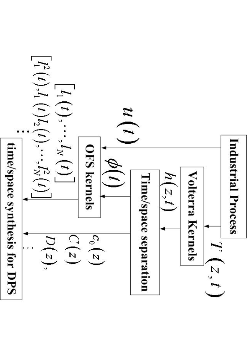
Figure 1: The sketch map of OFS-Volterra modeling for nonlinear DPS.

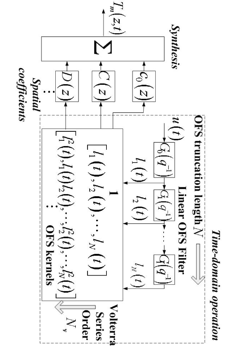
Figure 2: Operation details of OFS-Volterra modeling.

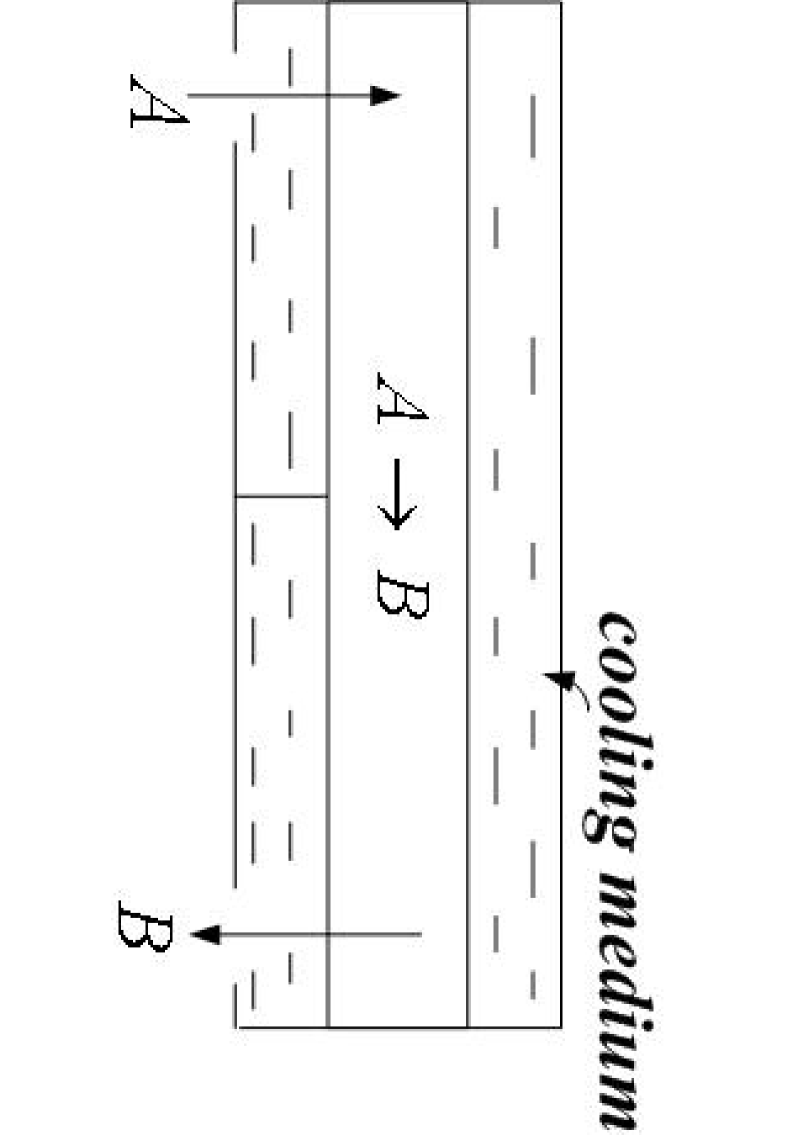
Figure 3: The sketch map of catalytic rod.

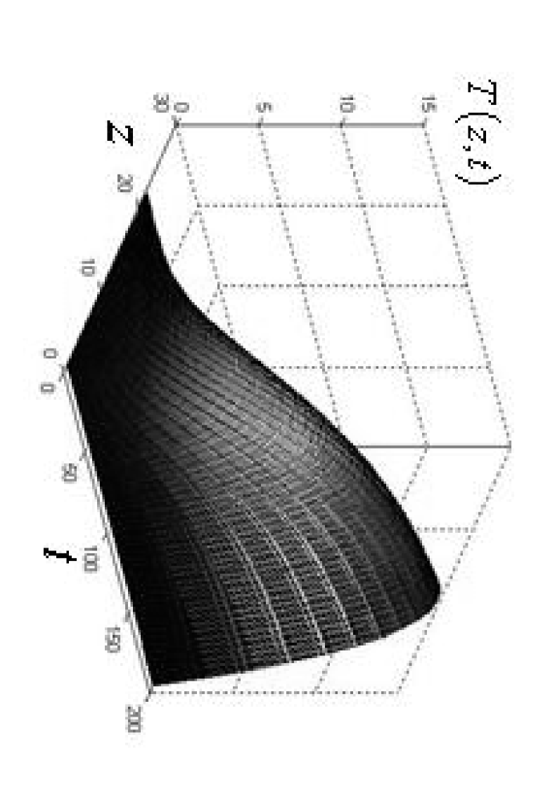
Figure 4: System output.

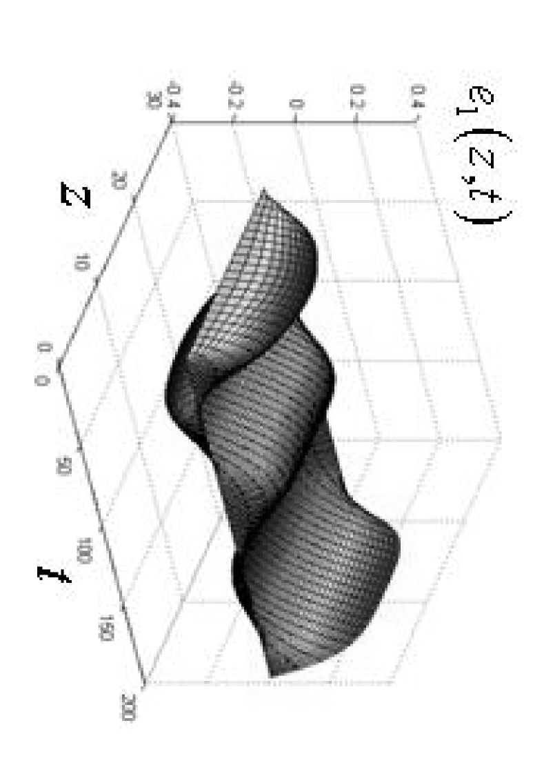
Figure 5: Modeling error of the traditional method.

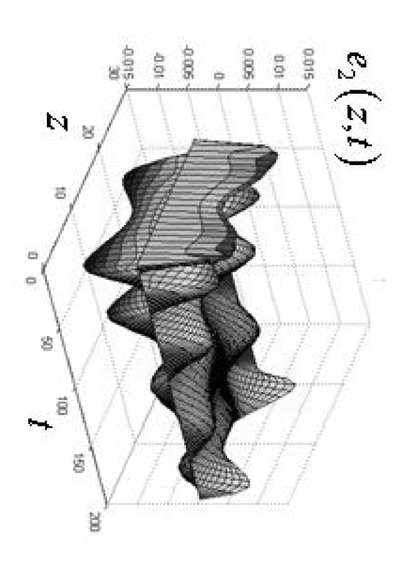
Figure 6: Modeling error of the present method.

Fig. 2 shows the operation details of this modeling method. The first order OFS filter is the Laguerre series, in which

$$G_{0}(q^{-1})=\frac{q^{-1}\sqrt{1-a^{2}}}{1-q^{-1}a},G_{1}(q^{-1})=\frac{q^{-1}-a}{1-q^{-1}a},$$ (6)

where $a$ is the time-scaling constant and $q^{-1}$ is the one step backward shifting operator (i.e. $q^{-1}u(t)=u(t-1)$). The second order OFS filter is the Kautz Series, in which $G_{0}(q^{-1})$ and $G_{1}(q^{-1})$ are second order transfer functions. Analogically, Heuberger et al. Heuberger1995 introduced the higher order OFS model. As the order increases, OFS model can handle more complex dynamics.

Numerical Results - Consider a long, thin rod in a reactor as shown in Fig. 3. The reactor is fed with pure species $A$ and a zeroth order exothermic catalytic reaction of the form $A\rightarrow B$ takes place in the rod. Since the reaction is exothermic, a cooling medium that is in contact with the rod is used for cooling. Assume the density, heat capacity, conductivity and temperature are all constant, and species $A$ is superfluous in the furnace, then the mathematical model which describes the spatiotemporal evolution of the rod temperature consists of the following parabolic partial differential equation:

$$\frac{\partial T}{\partial t}=\frac{\partial^{2}T}{\partial z^{2}}+\beta_{T}e^{-\frac{\gamma}{1+z}}-\beta_{T}e^{-\gamma}+\beta_{u}(b(z)u(t)-T),$$ (7)

which subjects to the Dirichlet boundary conditions:

$$T(0,t)=0,\texttt{ }T(\pi,t)=0,\texttt{ }T(z,0)=0,$$ (8)

where $T(z,t)$, $b(z)$, $\beta_{T}$, $\beta_{u}$, $\gamma$, and $u$ denote the temperature in the reactor (output), the actuator distribution function, the heat of reaction, the heat transfer coefficient, the activation energy, and the temperature of the cooling medium (input), respectively. Here we set $\beta_{T}=50.0$, $\beta_{u}=2.0$, and $\gamma=4.0$. In the numerical calculation, without loss of generality, we set $b(z)=1$, and $u(t)=[1.4,1.4,1.4,1.4]$. The order of Volterra series is two, the OFS is chosen as one-order Laguerre series Datta1995 with $a=0.6$, and the truncation length is given $N=4$.

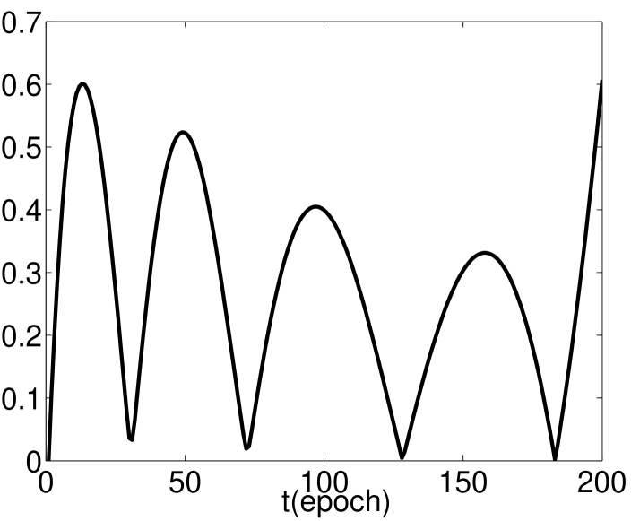
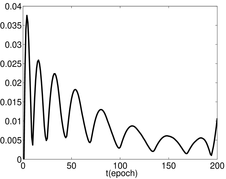
Figure 7: IAEs of the traditional method (left) and the present method (right).

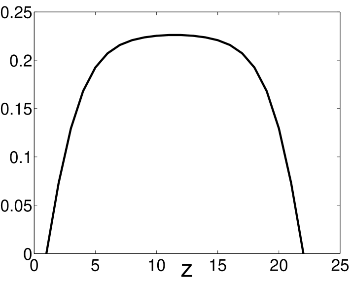
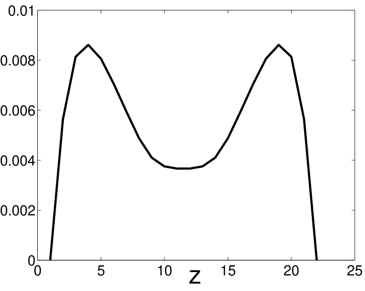
Figure 8: ITAEs of the traditional method (left) and the present method (right).

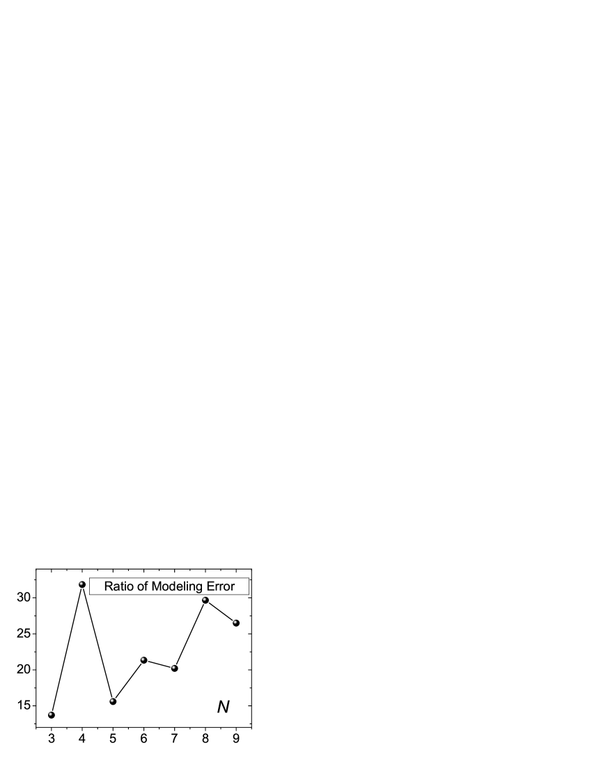
Figure 9: Ratios of the consumed time $t_{2}/t_{1}$ (left) and the average of absolute modeling error $|e_{1}|/|e_{2}|$ (right) vs the truncation length $N$. The subscripts 1 and 2 denote the cases of the traditional and the present methods, respectively. The CPU time by using traditional method for $N\in[3,9]$ is in the interval $[100s,160s]$. All the numerical calculations are implemented by using a personal computer with CPU: 1.8G, RAM: 256M, OS: Windows XP, and software platform: MATLAB 6.5.

The system output is shown in Fig. 4. Denote by $e(z,t)$ the modeling error, that is, the difference between system output and modeling result at the point $(z,t)$. Fig. 5 and Fig. 6 exhibit the modeling errors of the traditional and the present methods, respectively. Clearly, the method proposed here has remarkably smaller error than that of the traditional one. To provide a vivid contrast between these two methods, we calculate the integral of absolute error (IAE, $\int|e(z,t)|dz$) and time-weighted absolute errors (ITAE, $\int t|e(z,t)|dt$), which are two standard error indexes to evaluate modeling performances of DPS and can be considered as the modeling errors along the temporal dimension $t$ and the spatial dimension $z$. As are shown in Fig. 7 and Fig. 8, both the IAE and ITAE of the present method is reduced by $>20$ times comparing with those of the traditional one, which strongly demonstrates the advantage of the present method. Actually, to obtain the shapes of IAE and ITAE, one can cut the error surfaces of Figs. 5 and 6 along the temporal coordinate $t$ and the spatial dimension $z$. In addition, we calculate the average of absolute modeling error $\frac{1}{\int\int dzdt}\int\int|e(z,t)|dzdt$. From Fig. 9, it is found that, in comparison with the traditional method, the modeling accuracy of the present one is enhanced by 14-32 times with less than $15\%$ increase of the consumed time. It should be note that the modeling accuracy would increase along with the increase of the Volterra series order $N_{v}$, however, the computational complexity will increase too. For lumping systems, this fact has been proved, and for DPSs, this fact is also validated by experimental results Schetzen1980 . So a tradeoff between the modeling accuracy and the computational complexity must be made. That is why here we set the order $N_{v}=2$.

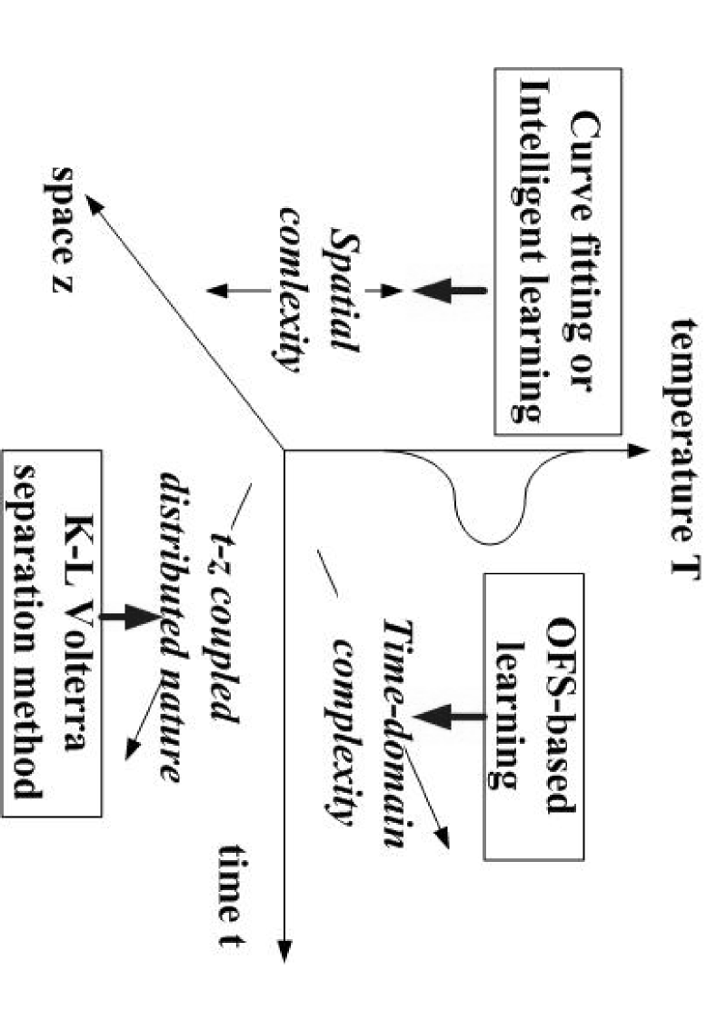
Figure 10: Modeling methodology for DPSs.

Conclusion and Discussion - Modeling method for nonlinear DPS plays an important role in physical system analysis and industrial engineering. Unfortunately, there exits two essential difficulties in this issue, a) distributed nature due to time-space coupled, which causes different temperature responses at different locations; b) nonlinear complexity from varying working point - different dynamics obtained even at the same location for a large change of working points. Owing to these difficulties, previous modeling methods via linear time/spatial separation techniques (e.g. KL approach, spectrum analysis, SVD-Galerkin technique, etc.) can not yield satisfying modeling performance, especially for DPSs with severe nonlinearity. The modeling error is caused by the nonlinear residue of the linear time/space separation. Thus, it is naturally to expect that a nonlinear time/space separation method may yield better modeling performance.

To validate this supposition, we design a novel modeling method by extending the concept of lumping Volterra series to the distributed scenario. As shown in Fig. 10, the nonlinear DPS is first decomposed into kernels, upon which the time-space separation is carried out. These two decompositions will gradually separate the complexity and provide a better modeling platform. The time/space separation will be handled by a novel KL Volterra method instead of the conventional KL method, the time-domain complexity by the OFS-based learning, and the spatial complexity by the curve fitting techniques (e.g. spline interpolation) or intelligent learning algorithms (e.g. neural network, fuzzy system, etc.). This novel method is applied on a benchmark nonlinear DPS of industrial process, a catalytic rod. It is found that the modeling accuracy is improved by more than 20 times in average comparing with the traditional method, with almost no additional computational complexity. The underlying reason may be that the high order Volterra kernel can compensate the residuals of the linear separation. In addition, we have applied this method to another two benchmark nonlinear DPSs, a rapid thermal chemical vapor deposition process Christofides2001 , and a Czochralski crystal growth process Christofides2001 . The corresponding results also strongly suggest that the nonlinear time/space separation can greatly enhance the modeling accuracy.

Although its superority has been demonstrated, the KL Volterra method is just a first attempt aiming at the motivation of nonlinear time/space separation. Thanks to its excellent modeling efficiency, this novel method is definitely a promising one for both physical system analysis and industrial engineering. We believe that our work can enlighten the readers on this interesting subject.

The author would like to thank Prof. Guanrong Chen for helpful discussion and suggestion. HTZhang would like to acknowledge the National Natural Science Foundation of China (NSFC) under Grant Nos. 60340420431 and 60274020, and the Youth Founding Project of HUST. TZhou would like to acknowledge NSFC under Grant Nos. 70471033, 10635040 and 70571074. HXLi would like to acknowledge the RGC-CERG founding of Hong Kong Government under Grant Nos. 9041015 and 9040916.

References

- (1) P. D. Christofides, Nonlinear and Robust Control of PDE systems: Methods and applications to transport-reaction processes (Boston, Birkhauser, 2001).
- (2) D. K. Hoffman, et al., Phys. Rev. E 57, 6152 (1998).
- (3) A. V. Chechkin, et al., Phys. Rev. E 66, 046129 (2002).
- (4) M. Sheintuch, and Y. Smagina, Phys. Rev. E 70, 026221 (2004).
- (5) P. V. Kuptsov, and R. A. Satnoianu, Phys. Rev. E 71, 015204 (2005).
- (6) W. J. Kossler, A. J. Greer, R. N. Dickes, D. Sicilia, and Y. Dai, Physica B 374-375, 225 (2006).
- (7) T. Yagi, N. Taketoshi, and H. Kato, Physica C 412-414, 1337 (2004).
- (8) V. A. Kazakov, and R. S. Berry, Phys. Rev. E 49, 2928 (1994).
- (9) M. I. Katsnelson, et al., Phys. Rev. A 62, 022118 (2000).
- (10) J. Wakabayashi, A. Tamagawa, T. Nagashima, T. Mochiku, and K. Hirata, Physica B 249-251, 102 (1998).
- (11) M. O. Vlad, and J. Ross, Phys. Rev. E 66, 061908 (2002).
- (12) U. Hass, Physica A 215, 247 (1995).
- (13) P. N. McGraw, and M. Menzinger, Phys. Rev. E 68, 066122 (2003).
- (14) W. H. Ray, Advanced Process Control (McGraw-Hill, New York, 1981).
- (15) H. M. Park, and D. H. Cho, Chemical Engineering Science 51, 81 (1996).
- (16) D. Gottlieb, and S. A. Orszag, Numerical analysis of spectral methods: Theory and applications (Philadelphia, SIAM, 1993).
- (17) S. Chakravarti, et al., Phys. Rev. E 52, 2407 (1995).
- (18) K. B. Datta, and B. M. Mohan, Orthogonal Functions in System and Control (World Scientific, 1995).
- (19) X. G. Hu, Phys. Rev. E 59, 2471 (2004).
- (20) C. de Boor, A Practical Guide to Splines (Springer-Verlag, 1978).
- (21) R. A. Sahan, et al., Proc. 1997 IEEE Int. Conf. Control Appl. (IEEE Press, pp. 359-364).
- (22) S. Y. Shvartsman, et al., J. Process Control 10, 177 (2000).
- (23) C. Canuto, M. Y. Hussaini, A. Quarteroni, and T. A. Zang, Spectral methods in fluid dynamics (Springer-Verlag, New York, 1988).
- (24) M. Schetzen, The Volterra and Wiener Theory of Nonlinear System (Wiley, New York, 1980).
- (25) S. Boyd, and L. O. Chua, IEEE Trans. Circuits and Systems 32, 1150 (1985).
- (26) V. A. Kuz, Phys. Rev. A 44, 8414 (1991).
- (27) I. Y. Cherdantsev, and R. I. Yamilov, Physica D 87, 140 (1995).
- (28) L. J. Chen, et al., Phys. Rev. E 50, 551 (1999).
- (29) L. P. Wang, Journal of Process Control 14, 131 (2004).
- (30) P. S. C. Heuberger, et al., IEEE Trans. Automatic Control 40, 451 (1995).