Edge pinch instability of liquid metal sheet in a transverse high-frequency ac magnetic field

Abstract

We analyze the linear stability of the edge of a thin liquid metal layer subject to a transverse high-frequency ac magnetic field. The layer is treated as a perfectly conducting liquid sheet that allows us to solve the problem analytically for both a semi-infinite geometry with a straight edge and a thin disk of finite radius. It is shown that the long-wave perturbations of a straight edge are monotonically unstable when the wave number exceeds the critical value $k_{c}=F_{0}/(\gamma l_{0}),$ which is determined by the linear density of the electromagnetic force $F_{0}$ acting on the edge, the surface tension $\gamma,$ and the effective arclength of edge thickness $l_{0}.$ Perturbations with wavelength shorter than critical are stabilized by the surface tension, whereas the growth rate of long-wave perturbations reduces as $\sim k$ for $k\rightarrow 0.$ Thus, there is the fastest growing perturbation with the wave number $k_{\max}=2/3k_{c}.$ When the layer is arranged vertically, long-wave perturbations are stabilized by the gravity, and the critical perturbation is characterized by the capillary wave number $k_{c}=\sqrt{g\rho/\gamma}$, where $g$ is the acceleration due to gravity and $\rho$ is the density of metal. In this case, the critical linear density of electromagnetic force is $F_{0,c}=2k_{c}l_{0}\gamma,$ which corresponds to the critical current amplitude $I_{0,c}=4\sqrt{\pi k_{c}l_{0}L\gamma/\mu_{0}}$ when the magnetic field is generated by a straight wire at the distance $L$ directly above the edge. By applying the general approach developed for the semi-infinite sheet, we find that a circular disk of radius $R_{0}$ placed in a transverse uniform high-frequency ac magnetic field with the induction amplitude $B_{0}$ becomes linearly unstable with respect to exponentially growing perturbation with the azimuthal wave number $m=2$ when the magnetic Bond number exceeds $\textrm{Bm}_{c}=B_{0}^{2}R_{0}^{2}/(2\mu_{0}l_{0}\gamma)=3\pi.$ For $\textrm{Bm}>\textrm{Bm}_{c},$ the wave number of the fastest growing perturbation is $m_{\max}=\left[2\textrm{Bm}/(3\pi)\right].$ These theoretical results agree well with the experimental observations.

I Introduction

In several induction melting processes, such as the cold crucible or electromagnetic levitation, liquid metal with a free surface is subject to ac magnetic fields that may cause considerable deformations of liquid metal resulting from the electromagnetic forces due to the eddy currents, which are often confined in a thin skin layer beneath the surface Sneyd-1993 . It has been observed that the free surface sometimes may become strongly asymmetric and even irregular when a sufficiently strong magnetic field is applied Perrier-etal-2003 ; Fautrelle-etal-2005 ; Mohring-etal-2005 .

Most of theoretical studies of the effect of ac magnetic field on the stability liquid metal surfaces have been concerned with flat surfaces subject to tangential uniform magnetic field. McHale and Melcher McHale-Melcher-1982 were the first to show that the time-averaged electromagnetic force has a destabilizing effect giving rise to traveling waves on the surface of liquid metal. Although the theoretical instability threshold is in good agreement with experimental results, the predicted growth rates are too small compared to the experimental observations. Note that such small growth rates are typical for the electromagnetic instabilities caused by the currents induced by motion of conducting media in ac magnetic fields Priede-Gerbeth-2005 . This simple model was revisited by a number of authors using various approximations. First, Garnier and Moreau Garnier-Moreau-1983 found that ac magnetic field has only a stabilizing effect on the surface waves when the currents induced by metal flow are neglected. Deepak and Evans Deepak-Evans-1995 took into account the motion of a surface but not the associated flow in the liquid, although both have a comparable effect, and they concluded that ac magnetic field can, however, give rise to unstable traveling surface waves. Stability of a flat metal layer suspended by means of a uniform magnetic field, as in the experiment of Hull et al. Hull-etal-1989 , has been studied by Ramos and Castellanos Ramos-Castellanos-1996 , who analyzed the effect of the viscosity on Rayleigh-Taylor type instability, which is unavoidable in this system. Fautrelle and Sneyd Fautrelle-Sneyd-1998 used a more elaborate model, taking into account not only the time-averaged but also the oscillating part of the electromagnetic force, which results in much stronger parametric instabilities when the frequency of surface waves is sufficiently close to the multiple of the electromagnetic force frequency. Note that this simple model of a flat surface with tangential magnetic field leads only to traveling but not stationary wave instabilities, which require consideration of nonplanar surfaces in nonuniform magnetic fields. A stability analysis was performed by Karcher and Mohring Karcher-Mohring-2003 to describe the experimental observations of static surface instabilities by Mohring et al. Mohring-etal-2005 . However, drastic simplifications were made in the latter analysis. First, the authors used the mirror image method to find the magnetic field distribution at the end of annular gap filled with liquid metal, however this method is applicable only to simple geometries, such as half-space or a sphere Jackson-75 . Second, they neglect the effect of surface perturbation on the magnetic field distribution, although the coupling between both constitutes the basic mechanism of this instability.

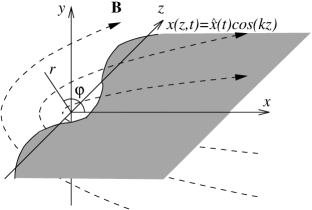
Figure 1: Sketch to the formulation of the problem with the magnetic flux lines (dashed) bending around perturbed edge $x(z,t)=\hat{x}(t)\cos(kz).$

In this work, we propose a simple theoretical model to describe such static surface instabilities. The model consists of a flat liquid metal layer in a transverse ac magnetic field. The ac frequency is assumed to be high so that the magnetic field is effectively expelled from the layer by the skin effect. The layer is assumed to be thin so that it can be regarded as a liquid perfectly conducting sheet. We start with the linear stability analysis of the straight edge of a semi-infinite liquid sheet, which allows us to work out a general approach, which is applied later to the liquid layer in the magnetic field of a straight wire parallel to the edge and to a thin circular liquid disk in a uniform transverse magnetic field. We describe a pinch-type instability of the edge of a liquid metal sheet with the following mechanism. The magnetic field bends around the edge of a perfectly conducting sheet, giving rise to the magnetic pressure on the edge, which tries to compress the sheet laterally. In the case of a straight edge, the uniform magnetic pressure along the edge is balanced by a constant pressure in the sheet. A wavelike perturbation of the edge causes the magnetic flux lines to diverge at wave crests and convergence at troughs. This redistribution is because the magnetic flux lines along the sheet are perpendicular to the electric current lines that are directed along the edge and, thus, the magnetic flux lines have to be perpendicular to the latter. As the result, the magnetic pressure is reduced at the crests and increased at the troughs, which enhances the perturbation.

The paper is organized as follows. In Sec. II, we consider the general model of a semi-infinite perfectly conducting liquid sheet with a straight edge, and compare with the experiment. In Sec. III, the linear stability problem for a thin disk in a transverse magnetic field is solved and compared with experiment. The results are summarized in Sec. IV.

II perfectly conducting liquid sheet

II.1 Mathematical model

Consider a thin layer of liquid metal submitted to a transverse ac magnetic field $B$. We assume that the layer is semi-infinite and lies on the right-hand side of $x$-$z$ plane, so that the unperturbed edge of the layer coincides with $z$ axis, as shown in Fig. 1. Field frequency is assumed to be high, so that the layer is effectively impermeable to the magnetic field because of the skin effect. In addition, the layer is assumed to be a thin sheet in a static equilibrium state supported by a flat horizontal non-wetting surface or constrained in the gap between two parallel walls. Note that this model represents a special case of a thin superconductor film (see, e.g., Brandt-1994 ). The magnetic field $B$ in the free space around the sheet can be described by the scalar magnetic potential $\Psi.$ Then the solenoidity constraint $\mbox{\boldmath$\nabla$}\cdot\mbox{\boldmath$B$}=0$ results in

$$\mbox{\boldmath$\nabla$}^{2}\Psi=0.$$ (1)

The impermeability condition at both sides of the sheet is

$$\left.\left(\mbox{\boldmath$n$}\cdot\mbox{\boldmath$B$}\right)\right|_{y=\pm 0;\,x>0}=\left.\frac{\partial\Psi}{\partial n}\right|_{y=\pm 0;\,x>0}=0,$$ (2)

where $n$ is the surface normal vector. First, we focus on the distribution of the magnetic field in the vicinity of the edge, which can conveniently be described in the cylindrical coordinates with the $z$ axis coinciding with the edge and the polar angle $\varphi$ measured from the $x$ axis, as illustrated in Fig. 1. The solution for the unperturbed potential in the vicinity of straight edge satisfying condition (2) is Landau-1984

$$\Psi_{0}(r,\varphi)=C_{0}\sqrt{r}\cos(\varphi/2),$$ (3)

where $C_{0}$ is an unknown constant. According to simple dimensional arguments, determining $C_{0}$ requires an external length scale that, however, is missing in this simple model. Thus, $C_{0}$ can be determined for a strip of finite width, a magnetic field generated by a straight wire placed at some distance parallel to the edge or a circular disk of finite size, that will be done in the following section. But first, we develop a general approach without specifying $C_{0}.$

Suppose that there is a perturbation of the edge position $x=x_{1}(z,t)=\hat{x}(t)\cos(kz)$ with a small, generally time-dependent amplitude $\hat{x}(t)$ and the wave number $k$ along the $z$ axis. This perturbation gives rise to the potential perturbation that can be presented as

$$\Psi(r,\varphi,z)=\Psi_{0}(r,\varphi)+\varepsilon\Psi_{1}(r,\varphi,z)+\cdots,$$

where $\Psi_{1}$ is a perturbation with small amplitude $\varepsilon.$ To relate the perturbation of a potential to that of the edge, we need an additional condition at the edge, which is derived as follows. For the surface current with density $J$, we have $\mu_{0}\mbox{\boldmath$J$}=\mbox{\boldmath$n$}\times\mbox{\boldmath$B$}$ Landau-1984 , where $\mu_{0}$ is the permeability of vacuum. According to this relation, the magnetic field along the sheet is perpendicular to the current. Consequently, the magnetic field has be to perpendicular to the edge because the current is flowing along the latter. Thus along the edge $L,$ we obtain $\left.\left(\mbox{\boldmath$\tau$}\cdot\mbox{\boldmath$B$}\right)\right|_{L}=\left.\partial\Psi/\partial\tau\right|_{L}=0,$ where $\tau$ is the unit vector tangential to the edge. This condition in turn implies that$\left.\Psi\right|_{L}=\mathrm{\mathit{const}},$ where $\mathrm{\mathit{const}}=0$ may be chosen because the potential is defined up to an additive constant. Applying this condition at the perturbed edge, we obtain up to the first-order terms in the perturbation amplitude

$$\left.\Psi\right|_{x=x_{1}}\approx\left.\left(\Psi_{0}+\frac{\partial\Psi_{0}}{\partial x}x_{1}+\varepsilon\Psi_{1}\right)\right|_{r\rightarrow 0;\,\varphi=0}=0,$$

which results in

$$\left.\varepsilon\Psi_{1}\right|_{r\rightarrow 0;\,\varphi=0}=-\left.\frac{\partial\Psi_{0}}{\partial x}x_{1}\right|_{r\rightarrow 0;\,\varphi=0}=-\left.\frac{C_{0}}{2}\frac{x_{1}}{\sqrt{r}}\right|_{r\rightarrow 0}.$$ (4)

Note that the base potential cannot formally be expanded in power series directly at the edge because the necessary derivative is singular there. To circumvent this, we take the expansion not exactly at the edge but define it as a limit when the expansion point approaches the edge.

The potential perturbation that satisfies Eq. (2) is of the same form as the base field $\hat{\Psi}_{1}(r,\varphi)=f_{1}(r)\cos(\varphi/2).$ When substituted into Eq. (1), this leads to

$$\frac{1}{r}\frac{d}{dr}\left(r\frac{df_{1}}{dr}\right)+\frac{1}{4}\frac{f_{1}}{r^{2}}-k{{}^{2}}f_{1}=0.$$

The solution satisfying Eq. (4) is $f_{1}(r)=-\frac{1}{2}C_{0}x_{1}e^{-kr}/\sqrt{r},$ and the full potential including the base field is

$$\Psi(r,\varphi,z)=C_{0}\sqrt{r}\left(1-\frac{1}{2}\frac{x_{1}}{r}e^{-kr}\cos(kz)\right)\cos(\varphi/2).$$ (5)

Note that the potential above, which is defined relative to the unperturbed edge, contains a singularity at the unperturbed edge. This singularity can be removed by proceeding to the coordinates defined relative to the perturbed edge as $\mbox{\boldmath$r$}=\mbox{\boldmath$r$}^{\prime}+\mbox{\boldmath$e$}_{x}x_{1},$ and expanding the solution in terms of $x_{1}.$ Thus, we obtain up to the first-order terms in the perturbation amplitude

$$\Psi(\mbox{\boldmath$r$}^{\prime}+\mbox{\boldmath$e$}_{x}x_{1}) \approx \left.\left(\Psi_{0}+\frac{\partial\Psi_{0}}{\partial x}x_{1}+\varepsilon\Psi_{1}\right)\right|_{\mbox{\boldmath$r$}=\mbox{\boldmath$r$}^{\prime}}$$

$$= C_{0}\sqrt{r^{\prime}}\left[1+\frac{x_{1}}{2r^{\prime}}\left[1-e^{-kr^{\prime}}\cos(kz)\right]\right],$$

where $r^{\prime}$ is the cylindrical radius relative to the perturbed edge. Having no singularity anymore, this solution simplifies in the vicinity of the edge to

$$\left.\Psi\right|_{r^{\prime}\rightarrow 0}\approx\tilde{C}_{0}\sqrt{r^{\prime}}\cos(\varphi/2),$$

where $\tilde{C}_{0}=C_{0}\left[1+\frac{1}{2}\hat{x}k\cos(kz)\right].$ Thus perturbation of the edge results just in a redefinition of the constant $C_{0},$ which is now replaced by $\tilde{C}_{0},$ whereas the distribution of the potential remains the same as for the straight edge obtained above. This is because a smoothly perturbed edge looks straight again when examined on a sufficiently small scale. The scalar magnetic potential in the vicinity of a straight edge and its perturbation amplitude defined by Eq. (II.1) are plotted in Fig. 2 with $1/k$ used as the length scale. The corresponding magnetic flux and current lines along the layer in the vicinity of the perturbed edge are shown in Fig. 3. As seen, the magnetic flux lines diverge at wave crests and converge at troughs in order to remain perpendicular to the edge, as discussed above. This redistribution of the magnetic flux lines at the perturbed edge is the principal physical mechanism behind the instability considered in this study.

Figure 2: Scalar magnetic potential in the vicinity of a straight edge (a) and its perturbation amplitude with $1/k$ used as the length scale (b).

Figure 3: Magnetic flux and current lines along the layer in the vicinity of the perturbed edge.

In the perfect conductor approximation, the electromagnetic force due to an ac magnetic field reduces to an effective magnetic pressure acting on the surface of the layer with the time-averaged value $p_{m}=\left|\mbox{\boldmath$B$}_{0}\right|^{2}/(4\mu_{0}),$ where $\mbox{\boldmath$B$}_{0}$ is the amplitude of an ac magnetic field. Note that part of the magnetic pressure, which oscillates with double ac frequency, is neglected here by assuming the frequency to be so high that inertia precludes any considerable reaction of the liquid. According to Eq. (5), the magnetic pressure increases toward the edge as $\sim 1/r$ and, thus, it becomes singular at $r=0$. Nevertheless, the integral force on the edge has a finite value. This is because the magnetic pressure at the edge of a layer of small but finite thickness $\sim d_{0}$ increases as $\sim 1/d_{0},$ which, integrated over the thickness, results in a finite value independent of $d_{0}$. The force on the edge can be evaluated by integrating the Maxwell stress tensor over a small cylindrical surface $S$ enclosing the edge, as shown in Fig. 4, that results in the first-order terms in

$$F = \frac{1}{2\mu_{0}}\lim_{r\rightarrow 0}\int_{0}^{2\pi}\left[-\frac{1}{2}\mbox{\boldmath$B$}^{2}\mbox{\boldmath$n$}+(\mbox{\boldmath$B$}\cdot\mbox{\boldmath$n$})\mbox{\boldmath$B$}\right]rd\varphi$$ (7)

$$= \mbox{\boldmath$e$}_{x}(F_{0}+F_{1}),$$

where

$$F_{0}=\frac{\pi C_{0}^{2}}{8\mu_{0}}$$ (8)

and $F_{1}=F_{0}k\hat{x}\cos(kz)$ are the base force and its perturbation, respectively.

Figure 4: Evaluation of the electromagnetic force on the edge by integration of the Maxwell stress tensor over a small cylindrical surface $S$ enclosing the edge.

Further, we assume the sheet to be an inviscid liquid, and consider a small-amplitude potential flow associated with the edge perturbation. Justification of this assumption, particularly at the threshold of monotonous instability, is discussed at the end of the section. Then the linearized Euler equation applied to a potential velocity field $\mbox{\boldmath$v$}=\mbox{\boldmath$\nabla$}\Phi,$

$$\rho\frac{\partial\mbox{\boldmath$v$}}{\partial t}+\mbox{\boldmath$\nabla$}p=\mbox{\boldmath$\nabla$}\left(\rho\frac{\partial\Phi}{\partial t}+p\right)=0,$$

leads to the pressure distribution in the sheet $p=p_{0}-\rho\partial\Phi/\partial t=p_{0}+p_{1},$ where $p_{0}$ is a constant base pressure and $p_{1}=-\rho\partial\Phi/\partial t$ is the perturbation of pressure. Velocity potential $\Phi$ is governed by the incompressibility constraint $\mbox{\boldmath$\nabla$}\cdot\mbox{\boldmath$v$}=0$ resulting in

$$\mbox{\boldmath$\nabla$}^{2}\Phi=0.$$ (9)

We integrate the normal stress balance over the edge by assuming both the pressure and curvature to be constant because of the small thickness of the layer, which yields

$$\left.p\right|_{x=0}=\frac{\gamma}{R}+\frac{F}{l_{0}},$$ (10)

where $l_{0}$ is the effective arclength of the edge thickness; $\gamma$ is the surface tension and $1/R$ denotes the curvature of the edge. For an unperturbed edge, we have $p_{0}=\gamma/R_{0}+F_{0}/l_{0}.$ Then for the perturbation, the balance condition takes the form

$$-\rho\left.\frac{\partial\Phi}{\partial t}\right|_{x=0}=\frac{\gamma}{R_{1}}+\frac{F_{1}}{l_{0}},$$ (11)

where $1/R_{1}\approx\mbox{\boldmath$\nabla$}^{2}x_{1}$ is the curvature perturbation of the edge. In addition, we have a kinematic constraint

$$\left.v_{x}\right|_{x=0}=\left.\frac{\partial\Phi}{\partial x}\right|_{x=0}=\frac{\partial x_{1}}{\partial t}.$$ (12)

Figure 5: Characteristic dependence of growth rate square scaled with its maximum value on the wave number.

Now we search for the amplitude of edge perturbation of the form $\hat{x}(t)=x_{0}e^{\lambda t},$ where $\lambda$ is, in general, a complex growth rate, whose real part has to be negative for the perturbation to be stable. The hydrodynamic potential is of the form

$$\Phi(x,z,t)=\hat{\Phi}(x)\cos(kz)e^{\lambda t},$$

which when substituted into Eq. (9) leads to $d^{2}\hat{\Phi}/dz^{2}-k^{2}\hat{\Phi}=0,$ whose solution decaying away from the edge is $\hat{\Phi}(x)=\Phi_{0}e^{-kx}.$ The amplitude of the hydrodynamic potential is related to that of the edge perturbation by the kinematic constraint (12) $\Phi_{0}=-x_{0}\lambda/k.$ Finally, the normal stress balance (11) yields the growth rate depending on the wave number

$$\lambda(k)=k\sqrt{\frac{1}{\rho}\left(\frac{F_{0}}{l_{0}}-k\gamma\right)},$$ (13)

which implies that long-wave perturbations with the wave numbers $0<k<k_{c}=F_{0}/(\gamma l_{0})$ have positive growth rates and, thus, they are unstable, as illustrated in Fig. 5. The stronger the electromagnetic force $F_{0}$ on the edge, the shorter the critical wavelength. The waves that are shorter than the critical one are stabilized by the surface tension. Although long waves are always unstable, their growth rate reduces as $\sim k$ for $k\rightarrow 0.$ Thus there is a perturbation with $k_{\max}=\frac{2}{3}k_{c}$ for which the growth rate attains the maximum $\lambda_{\max}=k_{\max}\sqrt{F_{0}/(3\rho l_{0})}$ (see Fig. 5).

Concerning the effect of neglected viscosity, simple physical arguments suggest that this instability can only be slowed down but not prevented by the viscosity. Note that the viscosity is inherently related to the fluid flow. But at the threshold of monotonous instability, where $\lambda(k_{c})=0,$ the characteristic time of monotonous instability tends to infinity. Consequently, there is no characteristic time and, thus, no characteristic velocity scale for the monotonous marginally stable mode which, therefore, cannot be affected by the viscosity.

II.2 Comparison with experiment

Figure 6: Magnetic flux lines and isolines of the scalar magnetic potential represented by the real and imaginary parts of the complex potential for a straight wire placed at $x=L=1$ and a semi-infinite sheet at $x<0$ (a) and for the sheet of finite height $-H<x<0$ transverse to a perfectly conducting wall at $x=-H=-2$ (b).

To compare our theory with the experiment of Mohring et al. Mohring-etal-2005 , similarly to Karcher-Mohring-2003 , we unfold the annular layer of InGaSn (Galinstan) melt used in experiment by approximating it by a semi-infinite flat perfectly conducting liquid sheet. Magnetic field is approximated by that of a straight wire lying at the distance $L$ from the edge in the plane of the sheet. The distance $L$ provides us with the length scale necessary to specify the constant $C_{0}$ used in our model above. This constant follows from the complex potential of the magnetic field, which is obtained by the conformal mapping

$$w(\zeta)=\frac{\mu_{0}I_{0}}{2\pi}\log\frac{\sqrt{\zeta}+\sqrt{L}}{\sqrt{\zeta}-\sqrt{L}},$$

where $\zeta=x+iy,$ as $C_{0}=\mu_{0}I_{0}/(\pi\sqrt{L}).$ The magnetic flux lines and isolines of the scalar magnetic potential represented by the real and imaginary part of this complex potential are shown in Fig. 6(a) with $L$ used as the length scale. In addition, we consider the gravity with the acceleration $\mbox{\boldmath$g$}=\mbox{\boldmath$e$}_{x}g$ directed downwards along the sheet normally to its edge. Then Eqs. (13) and (8) with $C_{0}$ defined above result in

$$\lambda(k)=k\sqrt{\frac{1}{\rho}\left(\frac{\mu_{0}I_{0}^{2}}{8\pi L_{0}l_{0}}-k\gamma\right)-\frac{g}{k}}.$$ (14)

Figure 7: Critical current amplitude vs the layer thickness. The circles correspond to the measured total current amplitude for the gap $L_{\mathrm{exp}}=17\,\mathrm{mm}$ between the metal surface and the lower side of the inductor Mohring-etal-2005 . The theoretical curve corresponds to the best fit with the effective gap with $L\approx 45\,\mathrm{mm}$ for a semi-infinite sheet and $L\approx 28\,\mathrm{mm}$ for a sheet of finite height $H=24\,\mathrm{mm}$ with a perfectly conducting bottom.

As is easy to see, the gravity stabilizes long-wave disturbances, whereas short waves are stabilized by the surface tension. Thus, the first unstable mode, defined by $\lambda(k_{c})=0,$ appears at the capillary wave number $k_{c}=\sqrt{\frac{g\rho}{\gamma}}\approx 0.296\,\mathrm{mm}^{-1}$ that corresponds to the critical wavelength $\Lambda_{c}=2\pi/k_{c}\approx 21.2\,\mathrm{mm},$ where $\rho=6440\,\mathrm{kq}/\mathrm{m}^{3}$ and $\gamma=0.718\,\mathrm{N}/\mathrm{m}$ are the density and surface tension of Galinstan Mohring-etal-2005 . Note that in the experiment, the surface of liquid metal is covered by a layer of NaOH solution. Thus, perturbation of the hydrostatic pressure at the interface is determined by the density difference of GaInSn and NaOH. Assuming the latter to have the density of water, we find the critical wavelength $\Lambda_{c}\approx 23\,\mathrm{mm}$ that coincides very well with that of the static surface deformation observed in the experiment. The critical electromagnetic force follows from Eq. (14) as $F_{0,c}=\sqrt{2\gamma l_{0}}/k_{c},$ which corresponds to the critical current amplitude

$$I_{0,c}=\pi\sqrt{\frac{8d_{0}L\sqrt{g\rho\gamma}}{\mu_{0}}},$$ (15)

where the edge arclength $l_{0}$ over the layer thickness $d_{0}$ is approximated by a half-circle, i.e., $l_{0}=\pi d_{0}/2.$ In order to compare this result with the measured critical currentsMohring-etal-2005 , note that the coil used in the experiment consists of two horizontal layers, each of which contains five windings. Thus, the measured current has to be multiplied by 10 to obtain the total current amplitude. Unfortunately, the authors do not specify the coil dimensions but give only the gap width $L_{\mathrm{exp}}=17\,\mathrm{mm}$ between the metal surface and the lower side of the inductor which is not sufficient for comparison with our theory. Therefore we treat the distance $L$ as a free parameter to fit the experimental results that yield $L\approx 45\,\mathrm{mm}$ (see Fig. 7). Note that the model of a semi-infinite layer may not be very adequate for the given experiment with the layer extention $H=24\,\mathrm{mm}$ which is comparable to the gap width $L$, especially when the layer resides on a well conducting metal plate. Finite extention of the layer and the conducting bottom can partly be accounted for by a more sophisticated complex potential,

$$w(\zeta)=\frac{\mu_{0}I_{0}}{2\pi}\log\frac{\sqrt{\zeta(\zeta+2H)}+\sqrt{L(L+2H)}}{\sqrt{\zeta(\zeta+2H)}-\sqrt{L(L+2H)}},$$

which is plotted in Fig. 6(b). This yields $C_{0}=\mu_{0}I_{0}/\left\{\pi\sqrt{L\left[1+L/(2H)\right]}\right\},$ resulting in $L\approx 28\,\mathrm{mm}$ which is considerably closer to the corresponding experimental value.

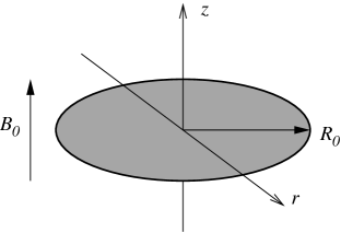
Figure 8: Sketch of a thin perfectly conducting disk in axial ac magnetic field.

III a thin liquid disk

III.1 Analytical solution

Now we will apply the approach developed in the previous section to a thin circular liquid disk of radius $R_{0}$ and fixed thickness $d_{0},$ which is subjected to a uniform axial ac magnetic field with an induction amplitude $B_{0},$ as shown in Fig. 8. The thickness $d_{0}$ is assumed to be small relative to the radius of disk $d_{0}\ll R_{0},$ so that the disk may be regarded as a thin sheet. The magnetic field is sought in terms of the scalar magnetic potential $\Psi$ governed by Eq. (1), whereas the impermeability condition at the disk surface $S$ takes the form

$$\left.\frac{\partial\Psi}{\partial n}\right|_{S}=0.$$ (16)

At large distances from the disk, the field is uniform and axial, which implies

$$\left.\Psi\right|_{\left|\mbox{\boldmath$r$}\right|\rightarrow\infty}\rightarrow(\mbox{\boldmath$r$}\cdot\mbox{\boldmath$B$}_{0})=zB_{0},$$ (17)

where $z$ is the axial distance from the disk. Solutions for both a circular and a slightly perturbed disk can be obtained analytically in the oblate spheroidal coordinates, which are related to the cylindrical ones by

$$r = R_{0}\sqrt{(1-\eta^{2})(1+\xi^{2})},$$

$$z = R_{0}\eta\xi,$$

where $0\leq\eta\leq 1$ and $0\leq\xi<\infty$ are the angular and radial spheroidal coordinates, respectively, as defined in Li-etal-2002 . Equation (1) for the unperturbed potential $\Psi_{0}$ around a circular disk takes the form

$$\frac{\partial}{\partial\eta}\left(\left(1-\eta^{2}\right)\frac{\partial\Psi_{0}}{\partial\eta}\right)+\frac{\partial}{\partial\xi}\left(\left(1+\xi^{2}\right)\frac{\partial\Psi_{0}}{\partial\xi}\right)=0.$$ (18)

The impermeability condition (16) is

$$\left.\frac{\partial\Psi_{0}}{\partial\xi}\right|_{\xi=0}=0.$$ (19)

The second boundary condition (17) suggests a solution of the form $\Psi_{0}(\eta,\xi)=\eta f_{0}(\xi).$ This results in Bojarevics-etal

$$\Psi_{0}(\eta,\xi)=C_{0}\eta\left[1+\xi\arctan(\xi)\right],$$ (20)

where $C_{0}=2R_{0}B_{0}/\pi,$ which is plotted in Fig. 9 with the corresponding magnetic flux lines. Note that in the vicinity of the edge this solution reduces to $\Psi_{0}=C_{0}\eta+O(\xi^{2}),$ which is equivalent to Eq. (3).

Figure 9: Isolines of the base magnetic potential $(r>0)$ and the corresponding magnetic flux lines $(r<0)$ around a circular disk.

Further, let us consider a perturbation of disk radius along the azimuthal angle $\phi$ of the form

$$R(\phi,t)=R_{0}+R_{1}^{m}(\phi,t),$$

where $R_{1}^{m}(\phi,t)=\hat{R}_{1}^{m}(t)\cos(m\phi)$ is a small perturbation with generally time-dependent amplitude $\hat{R}_{1}^{m}(t)$ for the wave number $m,$ which is integer in this case. Perturbation of the disk disturbs the magnetic potential as

$$\Psi(\eta,\xi,\phi,t)=\Psi_{0}(\eta,\xi)+\hat{\Psi}_{1}^{m}(\eta,\xi,t)\cos(m\phi)+\cdots,$$

where $\hat{\Psi}_{1}^{m}$ is the perturbation amplitude, which is associated with the wave number $m$, and satisfies the equation

$$\frac{\partial}{\partial\eta}\left(\left(1-\eta^{2}\right)\frac{\partial\hat{\Psi}_{1}^{m}}{\partial\eta}\right)+\frac{\partial}{\partial\xi}\left(\left(1+\xi^{2}\right)\frac{\partial\hat{\Psi}_{1}^{m}}{\partial\xi}\right)$$

$$-\frac{m^{2}\left(\eta^{2}+\xi^{2}\right)}{\left(1-\eta^{2}\right)\left(1+\xi^{2}\right)}\hat{\Psi}_{1}^{m}=0$$ (21)

Perturbation of the magnetic potential is related to that of the radius by the edge condition $\left.\Psi\right|_{r=R}=0$ resulting in

$$\left.\hat{\Psi}_{1}^{m}\right|_{\eta\rightarrow 0}=-\hat{R}_{1}^{m}\left.\frac{\partial\Psi_{0}}{\partial r}\right|_{r\rightarrow R_{0}}=\frac{\hat{R}_{1}^{m}}{R_{0}}\left.\frac{C_{0}}{\eta}\right|_{\eta\rightarrow 0}.$$ (22)

This perturbation vanishes with the distance from the disk, i.e., $\left.\hat{\Psi}_{1}^{m}\right|_{\xi\rightarrow\infty}\rightarrow 0.$ Although Eq. (21) admits variable separation, such a solution is complicated by the edge singularity (22). Nevertheless, a compact analytic solution can be found with the following original approach. First, note that if $\Psi$ is a solution of the Laplace equation and $\epsilon$ is a constant vector, $(\mbox{\boldmath$\epsilon$}\cdot\mbox{\boldmath$\nabla$})\Phi$ is a solution too. Second, if $\Psi$ satisfies a uniform boundary condition (16) and $\epsilon$ is directed along the boundary, $(\mbox{\boldmath$\epsilon$}\cdot\mbox{\boldmath$\nabla$})\Phi$ satisfies that boundary condition too. Third, the operator $(\mbox{\boldmath$\epsilon$}\cdot\mbox{\boldmath$\nabla$})$ changes the radial dependence of $\Psi$ from $\sim(r-R_{0})^{\alpha}$ to $\sim(r-R_{0})^{\alpha-1},$ while the azimuthal dependence is changed from mode $m$ to $m+1.$ Algebra becomes particularly simple when $\epsilon$ is defined in the complex form as $\mbox{\boldmath$\epsilon$}=\mbox{\boldmath$e$}_{x}+i\mbox{\boldmath$e$}_{y}=e^{i\phi}(\mbox{\boldmath$e$}_{r}+i\mbox{\boldmath$e$}_{\phi}).$ Then each application of the complex operator $(\mbox{\boldmath$\epsilon$}\cdot\mbox{\boldmath$\nabla$})\Phi$ is accompanied by the multiplication with $e^{i\phi}.$ Thus, the solution for $m=1$ follows simply from the axisymmetric basic state as

$$\hat{\Psi}_{1}^{1}(\eta,\xi) = -e^{-i\phi}C_{1}\left(\mbox{\boldmath$\epsilon$}\cdot\mbox{\boldmath$\nabla$}\right)\Psi_{0}$$

$$= C_{1}C_{0}\left(\frac{1-\eta^{2}}{1+\xi^{2}}\right)^{1/2}\frac{\eta}{\eta^{2}+\xi^{2}}.$$

Similarly, higher azimuthal modes can be found as $\hat{\Psi}_{1}^{m}=e^{-im\phi}\left(\mbox{\boldmath$\epsilon$}\cdot\mbox{\boldmath$\nabla$}\right)^{m}\hat{\Psi}_{0}^{m},$ where $\hat{\Psi}_{0}^{m}$ is an axisymmetric solution satisfying Eq. (18). From the edge condition

$$\left(\mbox{\boldmath$\epsilon$}\cdot\mbox{\boldmath$\nabla$}\right)^{m}\Psi_{0}^{m}\sim\frac{\Psi_{0}^{m}}{\eta^{2m}}\sim\frac{1}{\eta}$$

we obtain $\Psi_{0}^{m}\sim\eta^{2m-1}$ as $\eta\rightarrow 0.$ Moreover, vanishing of perturbation far away from the disk $\left.\hat{\Psi}_{1}^{m}\right|_{\xi\rightarrow\infty}\rightarrow 0$ implies that along the disk $\left.\hat{\Psi}_{0}^{m}\right|_{\xi=0}=c_{0}^{m}\eta^{2m-1},$ where $c_{0}^{m}$ is a constant. The corresponding axisymmetric solution of Eq. (18) can be represented as

$$\Psi_{0}^{m}(\eta,\xi)=c_{0}^{m}\sum_{k=1}^{m}c_{k}^{m}P_{2k-1}(\eta)Q_{2k-1}(i\xi),$$

where $P_{n}(x)$ and $Q_{n}(x)$ are the Legendre polynomials and functions of the second kind, respectively Abramowitz ; the expansion coefficients are $c_{k}^{m}=(4k-1)I_{k}^{m}/Q_{2k-1}(0),$ where

$$I_{k}^{m}=\int_{0}^{1}\eta^{2m-1}P_{2k-1}(\eta)d\eta=\frac{\sqrt{\pi}2^{1-2m}(2m-1)!}{(m-k)!\Gamma(m+k+1/2)}.$$

Then the solution for perturbation amplitude can be written as

$$\hat{\Psi}_{1}^{m}=D_{m-1}D_{m-2}\cdots D_{1}D_{0}\Psi_{0}^{m},$$ (23)

using the operator

$$D_{m}\equiv\frac{r}{R_{0}}\frac{1}{\eta^{2}+\xi^{2}}\left(-\eta\frac{\partial\,}{\partial\eta}+\xi\frac{\partial\,}{\partial\xi}\right)-\frac{mR_{0}}{r},$$

which is a spectral analog of $\left(\mbox{\boldmath$\epsilon$}\cdot\mbox{\boldmath$\nabla$}\right)$ acting on the azimuthal mode $m.$ Calculation of Eq. (23) is algebraically complicated but can be done using mathematica Mathematica , which requires a considerable amount computer memory and, thus, is possible only for $m\leq 5.$ Nevertheless, this suffices to deduce the general solution for arbitrary $m,$

$$\hat{\Psi}_{1}^{m}(\eta,\xi)=C_{m}C_{0}\left(\frac{1-\eta^{2}}{1+\xi^{2}}\right)^{m/2}\frac{\eta}{\eta^{2}+\xi^{2}},$$

where the unknown constant $C_{m}=\hat{R}_{1}^{m}/R_{0}$ follows from Eq. (22). It can easily be checked that the above solution indeed satisfies both Eq. (21) and the edge condition (22) as well as the impermeability condition (19). As for the semi-infinite sheet, the solution relative to the perturbed edge is obtained by the coordinate transformation

$$\Psi(\mbox{\boldmath$r$})=\Psi(\mbox{\boldmath$r$}^{\prime}+\mbox{\boldmath$e$}_{r}R_{1}^{m}) \approx \Psi_{0}(\mbox{\boldmath$r$}^{\prime})+\frac{\partial\Psi_{0}(\mbox{\boldmath$r$}^{\prime})}{\partial r}R_{1}^{m}+\Psi_{1}^{m}(\mbox{\boldmath$r$}^{\prime})$$

$$= \Psi_{0}(\mbox{\boldmath$r$}^{\prime})+\tilde{\Psi}_{1}^{m}(\mbox{\boldmath$r$}^{\prime})\cos(m\phi),$$

where $\tilde{\Psi}_{1}^{m}(\mbox{\boldmath$r$}^{\prime})=\hat{\Psi}_{1}^{m}(\mbox{\boldmath$r$}^{\prime})-\hat{\Psi}_{1}^{1}(\mbox{\boldmath$r$}^{\prime}).$ In the vicinity of the edge, this reduces to $\Psi(\eta,\xi)=\tilde{C}_{0}\eta+O(\xi^{2}),$ where $\tilde{C}_{0}=C_{0}\left[1-\frac{1}{2}(m-1)\hat{R}_{1}^{m}/R_{0}\right].$ Note that there is no perturbation of the magnetic field with respect to the edge for $m=1,$ because this mode corresponds to the offset of the disk as a whole. In this case, the field distribution moves together with the disk causing perturbation with respect to the original position of the disk, but not with respect to the disk itself. Perturbation amplitudes $\tilde{\Psi}_{1}^{m}(\mbox{\boldmath$r$}^{\prime})$ are plotted in Fig. 10 for modes $m=2$ and $3$.

Figure 10: Isolines of perturbation amplitudes of the magnetic potential relative to the perturbed edge for the azimuthal modes $m=2$ (a) and $m=3$ (b) plotted with the step $0.03$ for $C_{m}C_{0}=1.$

The time-averaged force on the edge follows from Eq. (7),

$$F=F_{0}+F_{1}=F_{0}\left(1-(m-1)\frac{R_{1}^{m}}{R_{0}}\right),$$

where $F_{0}=\pi C_{0}^{2}/(8\mu_{0}R_{0})=B_{0}^{2}R_{0}/(2\pi\mu_{0}).$ Similarly to the semi-infinite sheet, the normal stress balance at the edge of disk (10) results in

$$-\rho\left.\frac{\partial\Phi}{\partial t}\right|_{r=R_{0}}=K_{1}\gamma+\frac{F_{1}}{l_{0}},$$ (24)

where $\gamma$ is the surface tension of the disk. The hydrodynamic potential governed by Eq. (9) is found in cylindrical coordinates as $\Phi(r,\phi,t)=\hat{\Phi}_{m}(t)r^{m}\cos(m\phi),$ while the kinematic constraint $v_{r}=\left.\partial\Phi/\partial r\right|_{r=R_{0}}=\partial R_{1}^{m}/\partial t$ yields $\hat{\Phi}_{m}(t)=1/(mR_{0}^{m-1})d\hat{R}_{1}^{m}/dt.$ The curvature perturbation of the edge is

$$K_{1}=-\frac{R_{1}^{m}}{R_{0}^{2}}-\mbox{\boldmath$\nabla$}^{2}R_{1}^{m}=\frac{\hat{R}_{1}^{m}}{R_{0}^{2}}(m^{2}-1)\cos(m\phi).$$

Searching the edge perturbation as $\hat{R}_{1}^{m}(t)=R_{1}e^{\lambda_{m}t},$ where $\lambda_{m}$ is in general a complex growth rate of the azimuthal mode $m$, and substituting $\Phi$ and $K_{1}$ into Eq. (24), we eventually obtain

$$\lambda_{m}^{2}=\frac{m(m-1)}{\tau_{0}^{2}}\left(\frac{\textrm{Bm}}{\pi}-m-1\right),$$ (25)

where $\tau_{0}=\sqrt{\rho R_{0}^{3}/\gamma}$ is the characteristic time of capillary oscillations; $\textrm{Bm}=B_{0}^{2}R_{0}^{2}/(2\mu_{0}l_{0}\gamma)$ is the dimensionless magnetic Bond number characterizing the ratio of electromagnetic and surface tension forces. Without the magnetic field $(\textrm{Bm}=0),$ the growth rates for all modes are purely imaginary, $\lambda_{m}=\pm i(m-1)\sqrt{m},$ corresponding to capillary oscillations of an inviscid disk. Increasing the magnetic field results in a decrease of the frequency of oscillations until the critical value of Bm is attained, at which an exponentially growing mode appears. According to Eq. (25), the critical Bond number for mode $m,$ which is defined by the condition $\lambda_{m}(\textrm{Bm}_{c}^{m})=0$, is $\textrm{Bm}_{c}^{m}=(m+1)\pi,\,m=2,3,\ldots$. Note that for $m=0$ and $1,$ we have $\lambda_{m}=0$ regardless of Bm because the first mode is not permitted by the incompressibility constraint for the layer of fixed thickness under consideration here. The mode $m=1,$ as already noted above, corresponds to the offset of the disk as a whole, which has no effect relative to the disk itself as long as the external magnetic field is uniform. Thus, the first unstable mode is $m=2,$ for which the instability threshold is $\textrm{Bm}_{c}=3\pi.$ Similarly to the straight edge case considered above, when $\textrm{Bm}>\textrm{Bm}_{c}$ the growth rate attains a maximum at the wave number $m_{\max}$ defined by $\lambda_{m_{\max}}^{2}=\lambda_{m_{\max}-1}^{2}$ that yields $m_{\max}=\left[\frac{2}{3}\textrm{Bm}/\pi\right],$ where the square brackets denote the integer part.

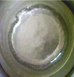
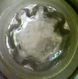
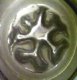
Figure 11: Top view of a flat Gallium drop in a transverse ac magnetic field of $13\,\mathrm{kHz}$ frequency at various induction amplitudes $B_{0}$: $12.9\,\mathrm{mT}$ (a), $23.5\,\mathrm{mT}$ (b), and $48.5\,\mathrm{mT}$ (c) .

III.2 Comparison with experiment

In the experiment, detailed description of which may be found in Perrier-etal-2003 , a flat circular gallium drop of thickness $d_{0}\approx 6\,\mathrm{mm}$ and radius $R_{0}\approx 30\,\mathrm{mm}$ was placed on a glass plate, which was slightly concave to center the drop, and put into a 6-winding solenoidal coil supplied by ac current of $f\approx 13\,\mathrm{kHz}$ frequency. At low currents in the coil, the drop was observed to be nearly circular, as seen in Fig. 11(a), and remained such until the current exceeded some critical value, after which the drop became noticeably distorted, as seen in Fig. 11(b). Further current increase resulted in the development of more corrugated drop shapes shown in Fig. 11(c). According to the experimental observations, the circular shape became unstable about the magnetic field induction amplitude in the range $12.9\,\mathrm{mT}<B_{0}<23.5\,\mathrm{mT}.$ Assuming the layer has approximately uniform curvature over the edge thickness with the radius $r_{0}\approx d_{0}/2$ that corresponds to an arclength $l_{0}\approx\pi d_{0}/2,$ we find $B_{0,c}=\sqrt{\pi\textrm{Bm}_{c}\mu_{0}\gamma d_{0}}/R_{0}\approx 13.4\,\mathrm{mT}$ for the critical Bond number $\textrm{Bm}_{c}=3\pi,$ where $\gamma=0.718\,\mathrm{N}/\mathrm{m}$ is the surface tension of gallium Smithells . This critical field strength is slightly higher than that in Fig. 11(a) but considerably lower than that in Fig. 11(b). For the latter case we have $\textrm{Bm}\approx 30,$ which corresponds to the critical wave number $m_{c}=\left[\textrm{Bm}/\pi\right]-1=8$ defining the range of linearly unstable modes $2\leq m\leq m_{c}.$ Note that the shape seen in Fig. 11(b) has $m\approx 8,$ which corresponds to the critical mode for the given Bond number, although the fastest growing mode in this case is $m_{\max}=6.$ Given the simplicity of our theoretical model, these results may be thought to agree well with the experiment. There may be several reasons that preclude a better agreement with the experiment. First, the drop seen in Fig. 11(b) has a significant perturbation amplitude implying that its shape may be affected by nonlinear effects that are not accounted for by this linear stability analysis. Second, our model of a thin perfectly conducting sheet may be too simple for the given experiment with the relative drop thickness $d_{0}/R_{0}\approx 0.2$ and the skin depth $\delta=1/\sqrt{\pi f\sigma\mu_{0}}\approx 2.3\,\mathrm{mm},$ where $\sigma=3.7\times 10^{6}\,\Omega^{-1}\mathrm{m}^{-1}$ is the electrical conductivity of gallium Smithells .

Note that our theory is developed for a disk of fixed thickness which excludes mode $m=0,$ while in the experiment the upper surface of the layer is free and this mode is permitted. Nevertheless, the theory is applicable also to this case because small-amplitude modes with $m\geq 1$ are not coupled with the mode $m=0.$ The only difference is that the thickness of the layer may vary depending on the magnetic field. But once the equilibrium thickness is known, our theory can be used to predict whether the droplet will remain circular on the further increase of the magnetic field.

IV Summary and conclusions

We have analyzed the linear stability of the edge of a thin liquid metal layer subject to a transverse high-frequency ac magnetic field. The metal layer was considered in the perfect conductor approximation supposing the ac frequency to be high so that the magnetic field is effectively expelled from the layer, while the thickness of the layer was assumed to be small relative to its lateral extension so that the layer could effectively be modeled as a thin perfectly conducting liquid sheet. First, we considered a general model of a semi-infinite sheet with a straight edge. This model, admitting an analytic solution, allowed us to identify a pinch-type instability of the edge with the following simple mechanism. The magnetic field bending around the edge of a perfectly conducting layer creates a magnetic pressure on the edge trying to compress the layer laterally. In the basic state with a straight edge, the magnetic pressure, which is uniform along the edge, is balanced by a constant hydrostatic pressure in the layer. Perturbation of the edge in the form of a wave causes divergence of magnetic flux lines at the wave crests and convergence in the troughs. This redistribution is because the magnetic flux lines along the sheet are perpendicular to the current lines. But since the latter are aligned along the edge, the magnetic field has to be perpendicular to it. Consequently, the magnetic pressure is reduced at the crests and increased at the troughs, which drives the instability. Note that in this model of a thin sheet, the induction varies with the distance $r$ from the edge as $\sim 1/\sqrt{r}$ and, thus, it formally becomes singular at the edge. We circumvented this singularity by considering the sheet to have a small but nevertheless finite thickness $d_{0}.$ Then integration of the magnetic pressure, which scales as $\sim 1/d_{0}$, over the thickness $d_{0}$ resulted in a finite integral force on the edge independent of its actual thickness. This allowed us to obtain an analytical solution showing that the long-wave perturbations are unstable when the wave number exceeds some critical value $k_{c}=F_{0}/(\gamma l_{0}),$ which is determined by the linear density of the electromagnetic force $F_{0}$ acting on the edge, the surface tension $\gamma,$ and the effective edge arclength $l_{0}$. The perturbations with wavelength shorter than critical are stabilized by the surface tension, whereas the growth rate of long-wave perturbations reduces as $\sim k$ for $k\rightarrow 0.$ Thus, there is the fastest growing perturbation with the wave number $k_{\max}=2/3k_{c}.$ When the layer is arranged vertically, long-wave perturbations are stabilized by the gravity, and the critical perturbation is characterized by the capillary wave number $k_{c}=\sqrt{g\rho/\gamma}.$ In this case, the critical linear density of electromagnetic force is $F_{0,c}=2k_{c}l_{0}\gamma,$ which corresponds to the critical current amplitude $I_{0,c}=4\sqrt{\pi k_{c}l_{0}L\gamma/\mu_{0}}$ when the magnetic field is generated by a straight wire at the distance $L$ directly above the edge. Next, we solved analytically the linear stability problem for a thin circular disk placed in a transverse uniform high-frequency ac magnetic field. It was found that the circular shape of the disk becomes unstable with respect to exponentially growing perturbation with the azimuthal wave number $m=2$ at the critical magnetic Bond number $\textrm{Bm}_{c}=3\pi.$ For $\textrm{Bm}>\textrm{Bm}_{c},$ the wave number of the fastest growing perturbation is $m_{\max}=\left[2\textrm{Bm}/(3\pi)\right].$ These theoretical results were found to be in reasonably good agreement with available experimental data.

- (1) A. D. Sneyd, IMA J. Math. Appl. Bus. Indust. 5, 87 (1993).
- (2) E. J. McHale and J. R. Melcher, J. Fluid Mech. 114, 276 (1982).
- (3) J. Priede and G. Gerbeth, IEEE Trans. Magn. 41, 2089 (2005).
- (4) M. Garnier, R. Moreau, J. Fluid Mech. 127, 365 (1983).
- (5) Deepak and J. W. Evans, J. Fluid Mech. 287, 133 (1995).
- (6) A. Ramos and A. Castellanos, Phys. Fluids 8, 1907 (1996).
- (7) J. R. Hull, T. Wiencek, and D. M. Rote, Phys. Fluids A 1, 1069 (1989).
- (8) Y. Fautrelle and A. D. Sneyd, J. Fluid Mech. 375, 65 (1998).
- (9) D. Perrier, Y. Fautrelle, and J. Etay, in Proceedings of the 4th International Conference on Electromagnetic Processing of Materials – EPM2003, Lyon, France, 2003, edited by S. Asai, Y. Fautrelle, P. Gillon, and F. Durand (EPM Madylam, St. Martin d’Hères; France, 2003), p. 279.
- (10) Y. Fautrelle, J. Etay, and S. Daugan, J. Fluid Mech. 527, 285 (2005).
- (11) J.-U. Mohring, Ch. Karcher, and D. Schulze, Phys. Rev. E 71, 047301 (2005).
- (12) Ch. Karcher and J.-U. Mohring, Magnetohydrodynamics 39, 267 (2003).
- (13) J. D. Jackson, Classical electrodynamics 2nd ed. (Wiley, New York, 1975).
- (14) E. H. Brandt, Phys. Rev. B 49, 9024; 50, 4034 (1994).
- (15) L. D. Landau and E. M. Lifshitz, Theoretical Physics, Vol. VIII: Electrodynamics of Continuous Media (Pergamon, Oxford, 1963).
- (16) A. Abramowitz and I. A. Stegun, Handbook of Mathematical Functions (Dover, New York, 1965).
- (17) L.-W. Li, X.-K. Kang, and M.-S. Leong, Spheroidal wave functions in electromagnetic theory (Wiley, New York, 2002)
- (18) V. Bojarevics, J. A. Freibergs, E. I. Shilova, E. V. Shcherbinin, Electrically Induced Vortical Flows (Kluwer, Dordrecht; Boston, 1989).
- (19) S. Wolfram, Mathematica: A System for Doing Mathematics by Computer (Addison-Wesley, Reading, MA, 1991).
- (20) Smithells Metals Reference Book, 7th ed., edited by E. A. Brandes and G. B. Brook (Butterworth-Heinemann, Oxford, 1997).