Instability and dynamics of two nonlinearly coupled laser beams in a plasma

Abstract

We investigate the nonlinear interaction between two laser beams in a plasma in the weakly nonlinear and relativistic regime. The evolution of the laser beams is governed by two nonlinear Schrödinger equations that are coupled with the slow plasma density response. We study the growth rates of the Raman forward and backward scattering instabilities as well of the Brillouin and self-focusing/modulational instabilities. The nonlinear evolution of the instabilities is investigated by means of direct simulations of the time-dependent system of nonlinear equations.

I Introduction

The interaction between intense laser beams and plasmas leads to a variety of different instabilities, including Brillouin and Raman forward and backward Shukla86 ; Sjolund67 ; Yu74 ; Shukla75 ; Shukla84 ; Tsintsadze74 scattering and modulational instabilities. In multiple dimensions we also have filamentation and side-scattering instabilities. Relativistic effects can then play an important role Shukla86 ; Tsintsadze74 ; Max74 . When two laser beams interact in the plasma, we have a new set of phenomena. An interesting application is the beat-wave accelerator, in which two crossing beams with somewhat different frequencies can accelerate electrons to ultra-relativistic speeds via the ponderomotive force acting on the electrons. The modulational and filamentation instabilities of multiple co-propagating electromagnetic waves can be described by a system of coupled nonlinear Schrödinger equations from which the nonlinear wave coupling and the interaction between localized light wave packets can be easily studied Shukla92 ; Berge98 . Two co-propagating narrow laser beams may attract each other and spiral around each other Ren01 or merge Dong02 . Counter-propagating laser beams detuned by twice the plasma frequency can, at relativistic intensities, give rise to fast plasma waves via higher-order nonlinearities Rosenbluth72 ; Shvets01 ; Bingham04 . At relativistic amplitudes, plasma waves can also be excited via beat wave excitation at frequencies different from the electron plasma frequency, with applications to efficient wake-field accelerators Shvets04 . The relativistic wakefield behind intense laser pulses is periodic in one-dimension Berezhiani90 and shows a quasi-periodic behavior in multi-dimensional simulations Tsung04 . Particle-in-cell simulations have demonstrated the generation of large-amplitude plasma wake-fields by colliding laser pulses Nagashima01 or by two co-propagating pulses where a long trailing pulse is modulated efficiently by the periodic plasma wake behind the first short pulse Sheng02 .

In the present paper, we consider the nonlinear interaction between two weakly relativistic crossing laser beams in plasmas. We derive a set of nonlinear mode coupled equations and nonlinear dispersion relations, which we analyze for Raman backward and forward scattering instabilities as well as for Brillouin and modulation/self-focusing instabilities.

II Nonlinear model equations

We consider the propagation of intense laser light in an electron–ion plasma. The slowly varying electron density perturbation is denoted by $n_{es1}$. Thus, our starting point is the Maxwell equation

$$\nabla\times\vec{B}=-\frac{4\pi}{c}(n_{0}+n_{es1})e\vec{v}+\frac{1}{c}\frac{\partial\vec{E}}{\partial t}.$$ (1)

The laser field is given in the radiation gauge, $\vec{B}=\nabla\times\vec{A}$ and $\vec{E}=-({1}/{c}){\partial\vec{A}}/{\partial t}$. Since $\partial\vec{p}_{e}/\partial t=-e\vec{E}$, we thus have $\vec{p}_{e}=e\vec{A}/c$. Moreover, $\vec{p}_{e}=m_{e}\gamma\vec{v}_{e}$, where $m_{e}$ is the electron rest mass and $\gamma=(1-v_{e}^{2}/c^{2})^{-1/2}$ is the relativistic gamma factor, so that

$$\vec{v}_{e}=\frac{e\vec{A}}{m_{e}c}\left(1+\frac{2e^{2}|\vec{A}|^{2}}{m_{e}^{2}c^{4}}\right)^{-1/2}.$$ (2)

For weakly relativistic particles, i.e. $e^{2}|\vec{A}|^{2}/m_{e}^{2}c^{4}\ll 1$, we can approximate (2) by

$$\vec{v}_{e}\approx\frac{e\vec{A}}{m_{e}c}\left(1-\frac{e^{2}|\vec{A}|^{2}}{m_{e}^{2}c^{4}}\right).$$ (3)

With these prerequisites, Eq. (1) becomes

$$\left(\frac{\partial^{2}}{\partial t^{2}}-c^{2}\nabla^{2}\right)\vec{A}+\omega_{\mathrm{p}0}^{2}\left(1+N_{s}\right)\vec{A}-\omega_{\mathrm{p}0}^{2}\frac{e^{2}|\vec{A}|^{2}}{m_{e}^{2}c^{4}}\vec{A}=0,$$ (4)

where $\omega_{\mathrm{p}0}=(4\pi n_{0}e^{2}/m_{e})^{1/2}$ is the electron plasma frequency and we have denoted $N_{s}=n_{es1}/n_{0}$.

Next, we divide the vector potential into two parts according to $\vec{A}=\vec{A}_{1}+\vec{A}_{2}$, representing the two laser pulses. We also consider the case $\vec{A}_{1}\cdot\vec{A}_{2}\approx 0$. With this, we obtain from (4) the two coupled equations

$$\left(\frac{\partial^{2}}{\partial t^{2}}-c^{2}\nabla^{2}\right)\vec{A}_{1}+\omega_{\mathrm{p}0}^{2}\left(1+N_{s}\right)\vec{A}_{1}-\omega_{\mathrm{p}0}^{2}\frac{e^{2}}{m_{e}^{2}c^{4}}(|\vec{A}_{1}|^{2}+|\vec{A}_{2}|^{2})\vec{A}_{1}=0,$$ (5a)

and

$$\left(\frac{\partial^{2}}{\partial t^{2}}-c^{2}\nabla^{2}\right)\vec{A}_{2}+\omega_{\mathrm{p}0}^{2}\left(1+N_{s}\right)\vec{A}_{2}-\\ \omega_{\mathrm{p}0}^{2}\frac{e^{2}}{m_{e}^{2}c^{4}}(|\vec{A}_{1}|^{2}+|\vec{A}_{2}|^{2})\vec{A}_{2}=0.$$ (5b)

Assuming that $A_{j}$ is proportional to $\exp(i\vec{k}_{j}\cdot\vec{r}-i\omega_{j}t)$ where $\omega_{j}\gg|\partial/\partial t|$, we obtain in the slowly varying envelope approximation two coupled nonlinear Schrödinger equations

$$-2i\omega_{1}\left(\frac{\partial}{\partial t}+\vec{v}_{g1}\cdot\nabla\right)\vec{A}_{1}-c^{2}\nabla^{2}\vec{A}_{1}+\omega_{\mathrm{p}0}^{2}N_{s}\vec{A}_{1}-\omega_{\mathrm{p}0}^{2}\frac{e^{2}}{m_{e}^{2}c^{4}}(|\vec{A}_{1}|^{2}+|\vec{A}_{2}|^{2})\vec{A}_{1}=0,$$ (6a)

and

$$-2i\omega_{2}\left(\frac{\partial}{\partial t}+\vec{v}_{g2}\cdot\nabla\right)\vec{A}_{2}-c^{2}\nabla^{2}\vec{A}_{2}+\omega_{\mathrm{p}0}^{2}N_{s}\vec{A}_{2}-\\ \omega_{\mathrm{p}0}^{2}\frac{e^{2}}{m_{e}^{2}c^{4}}(|\vec{A}_{1}|^{2}+|\vec{A}_{2}|^{2})\vec{A}_{2}=0,$$ (6b)

where $\vec{v}_{gj}=\vec{k}_{j}c^{2}/\omega_{j}$ is the group velocity and $\omega_{j}=(\omega_{p0}^{2}+c^{2}k_{j}^{2})^{1/2}$ is the electromagnetic wave frequency.

In order to close (6b), we next consider the slow plasma response. Here we may follow two routes. First, if we assume immobile ions, the slowly varying electron number density and velocity perturbations satisfy the equations

$$\frac{\partial n_{es1}}{\partial t}+n_{0}\vec{\nabla}\cdot\vec{v}_{es1}=0,$$ (7)

and

$$\frac{\partial\vec{v}_{es1}}{\partial t}+\frac{e^{2}}{m_{e}^{2}c^{2}}\vec{\nabla}(|\vec{A}_{1}|^{2}+|\vec{A}_{2}|^{2})=\frac{e}{m_{e}}\vec{\nabla}\phi_{s}-\frac{3T_{e}}{m_{e}n_{0}}\vec{\nabla}n_{es1}$$ (8)

where $T_{e}$ is the electron temperature, together with the Poisson equation

$$\nabla^{2}\phi_{s}=4\pi en_{es1}.$$ (9)

Thus, combining (7)–(9) together with the vector potential decomposition, we obtain

$$\left(\frac{\partial^{2}}{\partial t^{2}}-3v_{Te}^{2}\nabla^{2}+\omega_{\mathrm{p}0}^{2}\right)N_{s}=\frac{e^{2}}{m_{e}^{2}c^{2}}\nabla^{2}(|\vec{A}_{1}|^{2}+|\vec{A}_{2}|^{2}),$$ (10)

where the electron thermal velocity is denoted by $v_{Te}=(T_{e}/m_{e})^{1/2}$.

Second, if the electrons are treated as inertialess, we have in the quasi-neutral limit $n_{is1}=n_{es1}\equiv n_{s1}$

$$\frac{n_{0}e^{2}}{m_{e}c^{2}}\vec{\nabla}(|\vec{A}_{1}|^{2}+|\vec{A}_{2}|^{2})=n_{0}e\vec{\nabla}\phi_{s}-T_{e}\vec{\nabla}n_{s1},$$ (11)

and

$$n_{0}m_{i}\frac{\partial\vec{v}_{is1}}{\partial t}=-n_{0}e\vec{\nabla}\phi_{s}-3T_{i}\vec{\nabla}n_{s1}.$$ (12)

Adding Eqs. (11) and (12), we obtain

$$n_{0}m_{i}\frac{\partial\vec{v}_{is1}}{\partial t}+\frac{n_{0}e^{2}}{m_{e}c^{2}}\vec{\nabla}(|\vec{A}_{1}|^{2}+|\vec{A}_{2}|^{2})+(T_{e}+3T_{i})\vec{\nabla}n_{s1}=0,$$ (13)

which should be combined with

$$\frac{\partial n_{s1}}{\partial t}+n_{0}\vec{\nabla}\cdot\vec{v}_{is1}=0,$$ (14)

to obtain

$$\left(\frac{\partial^{2}}{\partial t^{2}}-c_{s}^{2}\nabla^{2}\right)N_{s}=\frac{e^{2}}{m_{e}m_{i}c^{2}}\nabla^{2}(|\vec{A}_{1}|^{2}+|\vec{A}_{2}|^{2}),$$ (15)

where the sound speed is $c_{s}=\sqrt{(T_{e}+3T_{i})/m_{i}}$ and $T_{i}$ is the ion temperature.

III Coupled laser beam amplitude modulation theory

We shall consider, successively, Eqs. (6a, b) combined with (10) (Case I: Raman scattering) or with (15) (Case II: Brillouin scattering).

III.1 Evolution equations

Setting $\nabla\rightarrow iK$ and $\partial/\partial t\rightarrow-i\Omega$ into the equations for the plasma density responses, we obtain

$$N_{s}=\alpha_{0}\,(|\vec{A}_{1}|^{2}+|\vec{A}_{2}|^{2})\,,$$ (16)

where,

for Case I:

$$\alpha_{0}=\frac{e^{2}}{m_{e}^{2}c^{2}}\,\,\frac{K^{2}}{\Omega^{2}-3K^{2}v_{Te}^{2}-\omega_{p0}^{2}}\,,$$ (17a)

and for Case II:

$$\alpha_{0}=\frac{e^{2}}{m_{e}m_{i}c^{2}}\,\,\frac{K^{2}}{\Omega^{2}-K^{2}c_{s}^{2}}\,.$$ (17b)

The expressions (16) and (17b) derived above provide the slow plasma response for any given pair of fields $\{\vec{A}_{j}\}$ ($j=1,2$). The latter now obey a set of coupled equations, which are obtained by substituting (16) into (6b),

$$2i\omega_{1}\left(\frac{\partial}{\partial t}+\vec{v}_{g1}\cdot\vec{\nabla}\right)\vec{A}_{1}+c^{2}\nabla^{2}\vec{A}_{1}+\omega_{\mathrm{p}0}^{2}\,\biggl{(}\frac{e^{2}}{m_{e}^{2}c^{4}}-\alpha_{0}\biggr{)}\,(|\vec{A}_{1}|^{2}+|\vec{A}_{2}|^{2})\vec{A}_{1}=0\,,$$ (18a)

and

$$2i\omega_{2}\left(\frac{\partial}{\partial t}+\vec{v}_{g2}\cdot\vec{\nabla}\right)\vec{A}_{2}+c^{2}\nabla^{2}\vec{A}_{2}+\omega_{\mathrm{p}0}^{2}\biggl{(}\frac{e^{2}}{m_{e}^{2}c^{4}}-\alpha_{0}\biggr{)}\,(|\vec{A}_{1}|^{2}+|\vec{A}_{2}|^{2})\vec{A}_{2}=0\,,$$ (18b)

For convenience, Eqs. (18ba) and (18bb) are cast into the reduced form as

$$2i\omega_{1}\left(\frac{\partial}{\partial t}+\vec{v}_{g1}\cdot\vec{\nabla}\right)\vec{A}_{1}+c^{2}\,\nabla^{2}\vec{A}_{1}+Q\,(|\vec{A}_{1}|^{2}+|\vec{A}_{2}|^{2})\vec{A}_{1}=0\,,$$ (19a)

and

$$2i\omega_{2}\left(\frac{\partial}{\partial t}+\vec{v}_{g2}\cdot\vec{\nabla}\right)\vec{A}_{2}+c^{2}\,\nabla^{2}\vec{A}_{2}+Q\,(|\vec{A}_{1}|^{2}+|\vec{A}_{2}|^{2})\vec{A}_{2}=0\,,$$ (19b)

where $\vec{A}_{j}$ has been normalized by $m_{e}c^{2}/e$ and where the nonlinearity/coupling coefficients are

$$Q=\omega_{p0}^{2}\biggl{(}1-\frac{K^{2}c^{2}}{\Omega^{2}-3K^{2}v_{Te}^{2}-\omega_{p0}^{2}}\biggr{)}\,,$$ (20a)

and

$$Q=\omega_{p0}^{2}\biggl{(}1-\frac{m_{e}}{m_{i}}\,\frac{K^{2}c^{2}}{\Omega^{2}-K^{2}c_{s}^{2}}\biggr{)}\,,$$ (20b)

for stimulated Raman (Case I) and Brillouin (Case II) scattering, respectively. We observe that the expressions (20ba) and (20bb) may be either positive or negative, depending on the frequency $\Omega$, prescribing either the modulational instability or the Raman and Brillouin scattering instabilities Tsintsadze79 .

The two nonlinear wave equations are identical upon an index ($1,2$) interchange, and coincide for equal frequencies $\omega_{1}=\omega_{2}$.

III.2 Nonlinear dispersion relation

We now investigate the parametric instabilities of the system of equations (19a) and (19b). Fourier decomposing the system by the ansatz $\vec{A}_{j}=[\vec{A}_{j0}+\vec{A}_{j+}\exp(i\vec{K}\cdot\vec{r}-i\Omega t)+\vec{A}_{j-}\exp(-i\vec{K}\cdot\vec{r}+i\Omega t))]\exp(-i\Omega_{0}t)$, where $|\vec{A}_{j0}|\gg|\vec{A}_{j\pm}|$, and sorting for different powers of $\exp(i\vec{K}\cdot\vec{r}-i\Omega t)$, we find the nonlinear frequency shift

$$\Omega_{j0}=-Q_{K=0}(|\vec{A}_{10}|^{2}+|\vec{A}_{20}|^{2})/2\omega_{j},$$ (21)

where $Q_{K=0}$ denotes the expression for $Q$ with $K=0$. For the nonlinear wave couplings, we have from (19b) the system of equations

$$D_{1+}X_{1+}+Q|A_{10}|^{2}(X_{1+}+X_{1+}+X_{2+}+X_{2-})=0,$$ (22a)

$$D_{1-}X_{1-}+Q|A_{10}|^{2}(X_{1+}+X_{1+}+X_{2+}+X_{2-})=0,$$ (22b)

$$D_{2+}X_{2+}+Q|A_{20}|^{2}(X_{1+}+X_{1+}+X_{2+}+X_{2-})=0,$$ (22c)

$$D_{1-}X_{1-}+Q|A_{20}|^{2}(X_{1+}+X_{1+}+X_{2+}+X_{2-})=0,$$ (22d)

where the unknowns are $X_{1+}=\vec{A}_{10}^{*}\cdot\vec{A}_{1+}$, $X_{1-}=\vec{A}_{10}\cdot\vec{A}_{1-}^{*}$, $X_{2+}=\vec{A}_{20}^{*}\cdot\vec{A}_{2+}$, and $X_{2-}=\vec{A}_{20}\cdot\vec{A}_{2-}^{*}$. The sidebands are characterized by

$$D_{j\pm}=\pm 2[\omega_{j}\Omega-c^{2}\vec{k}_{j}\cdot\vec{K}]-c^{2}K^{2},$$ (23)

where we have used $\vec{v}_{gj}=c\vec{k}_{j}/\omega_{j}$. The solution of the system of equations (22) yields the nonlinear dispersion relation

$$\frac{1}{Q}+\left(\frac{1}{D_{1+}}+\frac{1}{D_{1-}}\right)|\vec{A}_{10}|^{2}+\left(\frac{1}{D_{2+}}+\frac{1}{D_{2-}}\right)|\vec{A}_{20}|^{2}=0,$$ (24)

which relates the complex-valued frequency $\Omega$ to the wavenumber $\vec{K}$. Equation (24) covers Raman forward and backscattering instabilities, as well as the Brillouin backscattering instability or the modulational/self-focusing instability, depending on the two expressions for the coupling constant $Q$. If either $|\vec{A}_{10}|$ or $|\vec{A}_{20}|$ is zero, then we recover the usual expressions for a single laser beam in a laboratory plasma, or for a high-frequency radio beam in the ionosphere Stenflo90 .

IV Numerical results

We have solved the nonlinear dispersion relation (24) and presented the numerical results in Figs. 1–5. In all cases, we have used the normalized weakly relativistic pump wave amplitudes $A_{j0}=0.1$ with different sets of wavenumbers for the two beams. The nonlinear couplings between the laser beams and the Langmuir waves, giving rise to the Raman scattering instabilities (Case I), are considered in Figs. 1 and 2. The instability essentially obeys the matching conditions $\omega_{j}=\omega_{s}+\Omega$ and $\vec{k}_{j}=\vec{k}_{s}+\vec{K}$, where $\omega_{j}$ and $\vec{k}_{j}$ are the frequency and wavenumbers of the pump wave, $\omega_{s}$ and $\vec{k}_{s}$ are the frequency and wavenumbers for the scattered and frequency downshifted electromagnetic daughter wave, $\Omega$ and $K$ are the frequencies of the Langmuir waves, and where the light waves approximately obey the linear dispersion relation, $\omega_{j}=(\omega_{p0}^{2}+k_{j}^{2}c^{2})^{1/2}$, $\omega_{s}=(\omega_{p0}^{2}+k_{s}^{2}c^{2})^{1/2}$ and the low-frequency waves obey the Langmuir dispersion relation $\Omega=(\omega_{p0}^{2}+3K^{2}v_{Te}^{2})^{1/2}$. We thus have the matching condition $(\omega_{p0}^{2}+k_{j}^{2}c^{2})^{1/2}=[\omega_{p0}^{2}+(\vec{k}_{j}-\vec{K})^{2}c^{2}]^{1/2}+(\omega_{p0}^{2}+3K^{2}v_{Te}^{2})^{1/2}$, which in two-dimensions relates the components $K_{y}$ and $K_{z}$ of the Langmuir waves to each other, and which gives rise to almost circular regions of instability, as seen in Figs. 1 and 2. In the upper left and right panels of Fig. 1, we have assumed that the single beams $A_{1}$ and $A_{2}$ propagate in the $y$ and $z$ direction, respectively, having the wavenumber $(k_{1y},k_{1z})=(6,\,0)$ and $(k_{2y},\,k_{2z})=(0,\,4)$, respectively. We can clearly see a backward Raman instability, which for the beams $A_{1}$ and $A_{2}$ have maximum growth rates at $(K_{y},K_{z})=(2k_{1y},\,0)=(12,\,0)\,\omega_{p0}/c$ and $(K_{y},\,K_{z})=(0,\,2k_{2z})=(0,\,8)\,\omega_{p0}/c$, respectively. The backward Raman instability is connected via the obliquely growing wave modes to the forward Raman scattering instability that has a maximum growth rate (much smaller than that of the backward Raman scattering instability) at the wave number $K\approx\omega_{pe}/c$ in the same directions as the laser beams. In the lower panels, we consider the two beams propagating simultaneously in the plasma, at a right angle to each other (lower left panel) and in opposite directions (lower right panel). We see that the dispersion relation predicts a rather weak interaction between the two laser beams, where the lower left panel shows more or less a superposition of the growth rates in the two upper panels. The case of two counter-propagating laser beams (lower right panel) also shows a weak interaction between the two beams. For the case of equal wavelengths of the two pump waves, as shown in Fig. 2, we have a similar scenario as in Fig. 1. The lower left panel of Fig. 2 shows that the growth rate of two interacting laser beams propagating at a right angle to each other is almost a superposition of the growth rates of the single laser beams displayed in the upper panels of Fig. 2. Only for the counter-propagating laser beams in the lower right panel we see that the instability regions have split into broader and narrower bands of instability, while the magnitude of the instability is the same as for the single beam cases.

We next turn to the Brillouin scattering scenario (Case II), in which the laser wave is scattered against ion acoustic waves, displayed in Figs. 3 and 4. In the weakly nonlinear case, we have three-wave couplings in the same manner as for the interaction with Langmuir waves, and we see in both Figs. 3 and 4 that the instability has a maximum growth rate in a narrow, almost circular band in the $(K_{y},K_{z})$ plane. In the upper two panels, we also see the backscattered Brillouin instability with a maximum growth rate at approximately twice the pump wavenumbers, but we do not have the forward scattered instability. Instead, we see a broadband weak instability in all directions and also perpendicular to the pump wavenumbers. A careful study shows that the perpendicular waves are purely growing, i.e. there may be density channels created along the propagation direction of the laser beam. In the lower panels of Figs. 3 and 4, we display the cases with interacting laser beams. Also in the case of Brillouin scattering, the nonlinear dispersion relation predicts a rather weak interaction between the two beams, where the instability regions of the two beams are more or less superimposed without dramatic differences in the growth rates.

In order to investigate the nonlinear dynamics of the interacting laser beams in plasmas, we have carried out numerical simulations of the reduced system of equations (6b) in two spatial dimensions, and have presented the results in Figs. 5–8. In these simulations, we have used as an initial condition that either $A_{1}$ has a constant amplitude of $0.1$ and $A_{2}$ has a zero amplitude, or that both beams have a constant amplitude of $0.1$ and that they initially have group velocities at a right angle to each other. Due to symmetry reasons, it is sufficient to simulate one vector component of $\vec{A}_{j}$, which we will denote $A_{j}$ ($j=1,\,2$). The background plasma density is slightly perturbed with a low-level noise (random numbers). We first consider stimulated Raman scattering, displayed in Figs. 5 and 6. The single beam case in Fig. 5 shows a growth of density waves mainly in the direction of the beam, while a standing wave pattern is created in the amplitude of the electromagnetic wave envelope, where maxima in the laser beam amplitude is (roughly) correlated with minima in the electron density. This is in line with the standard Raman backscattering instability. The simulation is ended when the plasma density fluctuations are large and self-nonlinearities and kinetic effects are likely to become important. In Fig. 6, we show the case with the two beams crossing each other at a right angle. In this case, the wave pattern becomes slightly more complicated with local maxima of the laser beam envelope amplitude correlated with local minima of the electron density. However, this pattern is very regular and there is no clear sign of nonlinear structures in the numerical solution. We next turn to the case of stimulated Brillouin scattering, presented in Figs. 7 and 8. In this case, the waves grow not only in the direction of the laser beam but also, with almost the same growth rate, obliquely to the propagation direction of the laser beam. We see in the single beam case, presented in Fig. 7, that the envelope of the ion beam becomes modulated in localized areas both in $y$ and $z$ directions, and in the nonlinear phase at the end of the simulation, the laser beam envelope has local maxima correlated with local minima of the ion density. For the case of two crossed laser beams, displayed in Fig. 8, we see a more irregular structure of the instability and that at the final stage, local “hot spots” are created in which large amplitude laser beam envelopes are correlated with local depletions of the ion density.

V Summary

In summary, we have investigated the instability and dynamics of two nonlinearly interacting intense laser beams in an unmagnetized plasma. Our analytical and numerical results reveal that stimulated Raman forward and backward scattering instabilities are the dominating nonlinear processes that determine the stability of intense laser beams in plasmas, where relativistic mass increases and the radiation pressure effects play a dominant role. Our nonlinear dispersion relation for two interacting laser beams with different wavenumbers predicts a superposition of the instabilities for the single beams. The numerical simulation of the coupled nonlinear Schrödinger equations for the laser beams and the governing equations for the slow plasma density perturbations in the presence of the radiation pressures, reveal that in the case of stimulated Raman scattering, the nonlinear interaction between the two beams is weaker than for the case of stimulated Brillouin scattering. The latter case lead to local density cavities correlated with maxima in the electromagnetic wave envelope. The present results should be useful for understanding the nonlinear propagation of two nonlinearly interacting laser beams in plasmas, as well as for the acceleration of electrons by high gradient electrostatic fields that are created due to stimulated Raman scattering instabilities in laser-plasma interactions.

Figure captions

FIG. 1: The normalized (by $\omega_{p0}$) growth rates due to stimulated Raman scattering (Case I) for single laser beams (upper panels) and for two laser beams (lower panel), as a function of the wave numbers $K_{y}$ and $K_{z}$. The upper left and right panels show the growth rate for beam $\vec{A}_{1}$ and $\vec{A}_{2}$, respectively, where the wave vector for $\vec{A}_{1}$ is $(k_{y},\,k_{z})=(6,\,0)\,\omega_{p0}/c$ and the one for $\vec{A}_{2}$ is $(k_{y},\,k_{z})=(0,\,4)\,\omega_{p0}/c$, i.e. the two beams are launched in the $y$ and $z$ directions, respectively. In the lower left panel, $\vec{A}_{1}$ and $\vec{A}_{2}$ are launched simultaneously at a perpendicular angle to each other, and in the lower right panel, the two beams are counter-propagating. We used the normalized amplitudes $|\vec{A}_{10}|=|\vec{A}_{20}|=0.1$ and the electron thermal speed $v_{Te}=0.01c$.

FIG. 2: The normalized (by $\omega_{p0}$) growth rates due to stimulated Raman scattering (Case I) for single laser beams (upper panels) and for two laser beams (lower panel), as a function of the wave numbers $K_{y}$ and $K_{z}$. The upper left and right panels show the growth rate for beam $\vec{A}_{1}$ and $\vec{A}_{2}$, respectively, where the wavenumber for $\vec{A}_{1}$ is $(k_{y},\,k_{z})=(5,\,0)\,\omega_{p0}/c$ and the one for $\vec{A}_{2}$ is $(k_{y},\,k_{z})=(0,\,5)\,\omega_{p0}/c$. In the lower left panel, two beams are launched at a perpendicular angle to each other, and in the lower right panel, the two beams are counter-propagating. We used the normalized amplitudes $|\vec{A}_{10}|=|\vec{A}_{20}|=0.1$ and the electron thermal speed $v_{Te}=0.01c$.

FIG. 3: The normalized (by $\omega_{p0}$) growth rates due to stimulated Brillouin scattering (Case II) for single laser beams (upper panels) and for two laser beams (lower panel), as a function of the wave numbers $K_{y}$ and $K_{z}$. The upper left and right panels show the growth rate for the beam $\vec{A}_{1}$ and $\vec{A}_{2}$, respectively, where the wave number for $\vec{A}_{1}$ is $(k_{y},\,k_{z})=(6,\,0)\,\omega_{p0}/c$ and the one for $\vec{A}_{2}$ is $(k_{y},\,k_{z})=(0,\,4)\,\omega_{p0}/c$. In the lower left panel, two beams are launched at a perpendicular angle to each other, and in the lower right panel, the two beams are counter-propagating. We used the normalized amplitudes $|\vec{A}_{10}|=|\vec{A}_{20}|=0.1$, the ion to electron mass ratio $m_{i}/m_{e}=73440$ (Argon), and the ion sound speed $c_{s}=3.4\times 10^{-5}\,c$.

FIG. 4: The normalized (by $\omega_{p0}$) growth rates due to stimulated Brillouin scattering (Case II) for single laser beams (upper panels) and for two laser beams (lower panel), as a function of the wave numbers $K_{y}$ and $K_{z}$. The upper left and right panels show the growth rate for beam $\vec{A}_{1}$ and $\vec{A}_{2}$, respectively, where the wavenumber for $\vec{A}_{1}$ is $(k_{y},\,k_{z})=(5,\,0)\,\omega_{p0}/c$ and the one for $\vec{A}_{2}$ is $(k_{y},\,k_{z})=(0,\,5)\,\omega_{p0}/c$. In the lower left panel, two beams are launched at a perpendicular angle to each other, and in the lower right panel, the two beams are counter-propagating. We used the normalized amplitudes $|\vec{A}_{10}|=|\vec{A}_{20}|=0.1$, the ion to electron mass ratio $m_{i}/m_{e}=73440$ (Argon), and the ion sound speed $c_{s}=3.4\times 10^{-5}\,c$.

FIG. 5: The amplitude of a single laser beam $|A_{1}|$ (left panels) and the electron density $N_{s}$ (right panels) involving stimulated Raman scattering (Case I), at times $t=1.0\,\omega_{p0}^{-1}$, $t=30\,\omega_{p0}^{-1}$ and $t=60\,\omega_{p0}^{-1}$ (upper to lower panels). The laser beam initially has the amplitude $A_{1}=0.1$ and wavenumber $(k_{1y},\,k_{1z})=(0,\,5)\,\omega_{p0}/c$. The electron density is initially perturbed with a small-amplitude noise (random numbers) of order $10^{-4}$.

FIG. 6: The amplitude of two crossed laser beams, $|A|=(|A_{1}|^{2}+|A_{2}|^{2})^{1/2}$ (left panels) and the electron density $N_{s}$ (right panels) involving stimulated Raman scattering (Case I), at times $t=1.0\,\omega_{p0}^{-1}$, $t=30\,\omega_{p0}^{-1}$ and $t=60\,\omega_{p0}^{-1}$ (upper to lower panels). The laser beams initially have the amplitude $A_{1}=A_{2}=0.1$, and $A_{1}$ initially has the wavenumber $(k_{1y},\,k_{1z})=(0,\,5)\,\omega_{p0}/c$ while $A_{2}$ has the wavenumber $(k_{2y},\,k_{2z})=(5,\,0)\,\omega_{p0}/c$. The electron density is initially perturbed with a small-amplitude noise (random numbers) of order $10^{-4}$.

FIG. 7: The amplitude of a single laser beam $|A_{1}|$ (left panels) and the electron density $N_{s}$ (right panels) involving stimulated Brillouin scattering (Case II), at times $t=1.5\,\omega_{p0}^{-1}$, $t=600\,\omega_{p0}^{-1}$ and $t=1200\,\omega_{p0}^{-1}$ (upper to lower panels). The laser beam initially has the amplitude $A_{1}=0.1$ and wavenumber $(k_{1y},\,k_{1z})=(0,\,5)\,\omega_{p0}/c$. The ion density is initially perturbed with a small-amplitude noise (random numbers) of order $10^{-4}$.

FIG. 8: The amplitude of two crossed laser beams, $|A|=(|A_{1}|^{2}+|A_{2}|^{2})^{1/2}$ (left panels) and the electron density $N_{s}$ (right panels) involving stimulated Brillouin scattering (Case II), at times $t=1.0\,\omega_{p0}^{-1}$, $t=30\,\omega_{p0}^{-1}$ and $t=60\,\omega_{p0}^{-1}$ (upper to lower panels). The laser beams initially have the amplitude $A_{1}=A_{2}=0.1$, and $A_{1}$ initially has the wavenumber $(k_{1y},\,k_{1z})=(0,\,5)\,\omega_{p0}/c$ while $A_{2}$ has the wavenumber $(k_{2y},\,k_{2z})=(5,\,0)\,\omega_{p0}/c$. The electron density is initially perturbed with a small-amplitude noise (random numbers) of order $10^{-4}$.

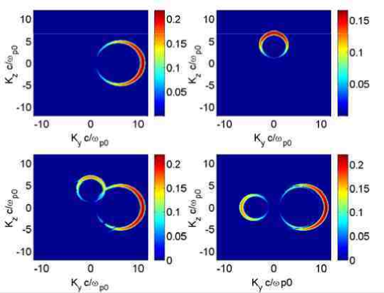
Figure 1:

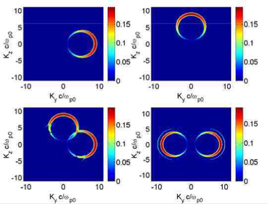
Figure 2:

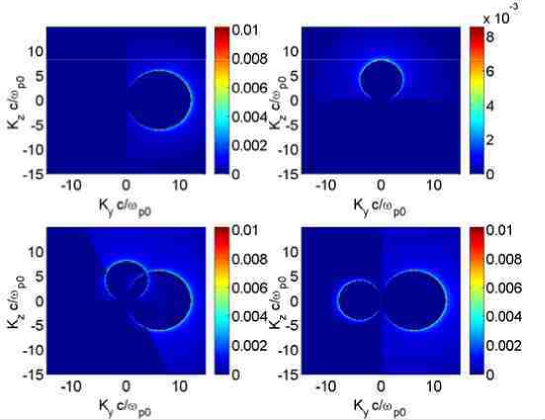
Figure 3:

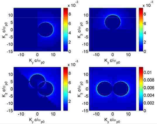
Figure 4:

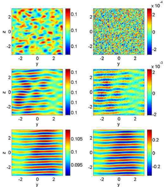
Figure 5:

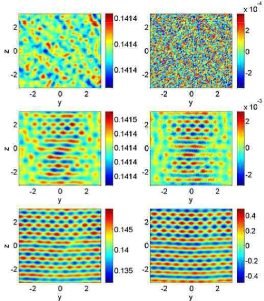
Figure 6:

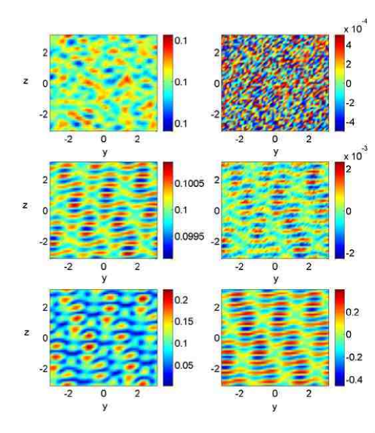
Figure 7:

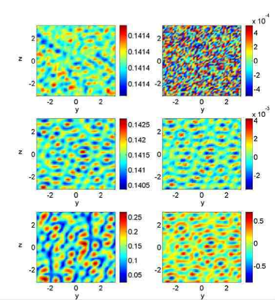
Figure 8:

References

(1) P. K. Shukla, N. N. Rao, M. Y. Yu, and N. L. Tsintsadze,
Phys. Rep. 135, 1 (1986).
(2) A. Sjölund and L. Stenflo, Appl. Phys. Lett. 10,
201 (1967).
(3) M. Y. Yu, K. H. Spatschek, and P. K. Shukla, Z. Naturforsch. A 29, 1736 (1974).
(4) P. K. Shukla, M. Y. Yu, and K. H. Spatschek, Phys. Fluids 18, 265 (1975).
(5) P. K. Shukla and L. Stenflo, Phys. Rev. A 30, 2110 (1984).
(6) N. L. Tsintsadze and L. Stenflo,
Phys. Lett. A 48, 399 (1974).
(7) C. E. Max, J. Arons, and A. B. Langdon,
Phys. Rev. Lett. 33, 209 (1974).
(8) P. K. Shukla, Phys. Scripta 45, 618 (1992).
(9) L. Bergé, Phys. Rev. E 58, 6606 (1998).
(10) C. Ren, B. J. Duda, and W. B. Mori, Phys. Rev. E 64, 067401 (2001).
(11) Q.-L. Dong, Z.-M. Sheng, and J. Zhang,
Phys. Rev. E 66, 027402 (2002).
(12) M. N. Rosenbluth and C. S. Liu, Phys. Rev. Lett.
29, 701 (1972).
(13) G. Shvets and N. J. Fisch, Phys. Rev. Lett. 86,
3328 (2001).
(14) R. Bingham, J. T. Mendonça and P. K. Shukla, Plasma Phys. Control. Fusion 46, R1 (2004).
(15) G. Shvets, Phys. Rev. Lett. 93, 195001 (2004).
(16) V. I. Berezhiani and I. G. Murusidze,
Phys. Lett. A 148, 338 (1990).
(17) F. S. Tsung, R. Narang, W. B. Mori, R. A. Fonseca, and
L. O. Silva, Phys. Rev. Lett. 93, 185002 (2004).
(18) K. Nagashima, J. Koga, and M. Kando, Phys. Rev. Lett.
64, 066403 (2001).
(19) Z.-M. Sheng, K. Mima, Y. Setoku, K. Nishihara, and
J. Zhang, Phys. Plasmas 9, 3147 (2002).
(20) N. L. Tsintsadze, D. D. Tskhakaya, and L. Stenflo,
Phys. Lett. A 72, 115 (1979).
(21) L. Stenflo, Phys. Scripta T30, 166 (1990);
ibidT107, 262 (2004).