Mean number of visits to sites in Levy flights

Abstract

Formulas are derived to compute the mean number of times a site has been visited during symmetric Levy flights. Unrestricted Levy flights are considered first, for lattices of any dimension: conditions for the existence of finite asymptotic maps of the visits over the lattice are analysed and a connection is made with the transience of the flight. In particular it is shown that flights on lattices of dimension greater than one are always transient. For an interval with absorbing boundaries the mean number of visits reaches stationary values, which are computed by means of numerical and analytical methods; comparisons with Monte Carlo simulations are also presented.

I Introduction

Levy flights are a model of diffusion in which the probability of a $|z|$-length jump is “broad”, in that, asymptotically, $p(z)\sim|z|^{-1-\alpha}$, $0<\alpha<2$. In this case the sum $x_{k}=\sum_{i}^{k}z_{i}$ is distributed according to a Levy distribution, whereas for $\alpha\geq 2$ normal diffusion takes place bib:gnko , bib:boge . Interesting problems arise in the theory of Levy flights when considering the statistics of the visits to the sites, such for instance the number of different sites visited during a flight bib:giwe , bib:boha ; in this paper we consider a different, but related, problem, namely the number of times a site visited by a random flyer.

Suppose that a random walk takes place on a $d$-dimensional lattice $\mathcal{L}$, let ${\bf s}$ be a site of $\mathcal{L}$ and let $P^{(d)}_{k}({\bf s})$ be the probability that after $k$ steps the walker is at ${\bf s}$. The mean value of visits to the site ${\bf s}$ after $n$ steps is bib:feza

$$M^{(d)}_{n}({\bf s})=\sum_{k=0}^{n}P^{(d)}_{k}({\bf s});$$ (1)

since derivation of Eq. (1) does not depend on the specific form of the walk bib:feza , it holds also for Levy flights. In the following it will be assumed $M_{0}({\bf s})=P_{0}({\bf s})=\delta_{{\bf s},0}$; the asymptotic value of $M^{(d)}_{n}$, denoted by ${\mathcal{M}}^{(d)}$, is defined as ${\mathcal{M}}^{(d)}=\lim_{n\rightarrow\infty}M^{(d)}_{n}$. It is known bib:fel that a random walk is transient if and only if $\sum_{k=0}^{\infty}P^{(d)}_{k}({\bf s})<\infty$; in other words the existence of finite ${\mathcal{M}}^{(d)}$ implies that the walk is transient.

Levy flights have a wide range of applications (see for instance bib:ch and references therein) and, in particular, analysis of the number of times a site is visited can be relevant in those processes, such as random searches, in which it is important not just to determine what sites have been visited but how often they have been visited; examples of possible applications range from animal foraging bib:visw to exploration of visual space bib:bocfer . Moreover $M_{n}^{(d)}$ can be given the following interpretation, useful for possible applications: assume that particles undergoing a Levy flight are continuously generated at the origin, then, at time $n$, $M_{n}^{(d)}({\bf s})\propto C_{n}^{(d)}({\bf s})$, where $C_{n}^{(d)}({\bf s})$ is the mean number of particles at site ${\bf s}\neq 0$ bib:fzpha . This property of $M^{(d)}_{n}$ has been used, in a model based on electrons Brownian motion, to simulate distributions of emissivity of supernova remnants bib:fzpha .

II Infinite lattices

Consider first one-dimensional, infinite lattices; the probability of occupancy of site $x$ after $k$ steps is bib:hsm

$$P^{(1)}_{k+1}(x)=\sum_{x=-\infty}^{\infty}p(x-y)P^{(1)}_{k}(y),$$ (2)

where $p(y)$ is the probability of having a displacement of $y$ sites. In case of symmetric Levy flights the canonical representation of $p$ and $P^{(1)}_{k}$ are bib:gnko , bib:boge

$$p(y)=\frac{1}{\pi}\int_{0}^{\infty}\cos qy\exp(-cq^{\alpha})dq,$$ (3)

$$P^{(1)}_{k}(x)=\frac{1}{\pi}\int_{0}^{\infty}\cos qx\exp(-ckq^{\alpha})dq,$$ (4)

where $0<\alpha<2$ and $c$ is a real number, which in the following will be set equal to 1 for simplicity bib:boge ; a scaling relation holds between $P^{(1)}_{k}$ and $p$, namely $P^{(1)}_{k}(x)=k^{-1/\alpha}p(xk^{-1/\alpha})$. If $\alpha=2$ Eqs. (3), (4) yield the Gaussian distribution bib:gnko , bib:fel , whereas, if $\alpha>2$, $P^{1}_{k}$ fails to be a proper distribution not concentrated at a point bib:fel ; therefore representations (3), (4) are valid only in the interval $0<\alpha\leq 2$. More recently it has been shown that the analytic forms of $p$ and $P^{(1)}_{k}$ can be given through a Fox function bib:mekl .

Application of (1) and of the scaling relation leads to $M^{(1)}_{n}(x)=\delta_{x,0}+\sum_{k=1}^{n}k^{-\frac{1}{\alpha}}p\left(\frac{x}{k^{1/\alpha}}\right)$, and in particular, recalling that $p(0)=(\pi\alpha)^{-1}\Gamma(1/\alpha)$ bib:boge ,

$$M^{(1)}_{n}(0)=1+\frac{\Gamma(1/\alpha)}{\pi\alpha}\sum_{k=1}^{n}k^{-\frac{1}{\alpha}},$$ (5)

with $\sum_{k=1}^{n}k^{-1/\alpha}$ converging to a finite value for $n\rightarrow\infty$ if and only if $\alpha<1$ bib:abst ; in this case

$${\mathcal{M}}^{(1)}(0)=1+\frac{\Gamma(1/\alpha)}{\pi\alpha}\zeta(1/\alpha),$$ (6)

where $\zeta$ is the well known Riemann zeta function bib:abst . Thus Eqs. (5) and (6), show that the visit to site $x=0$ is a transient state if and only if $\alpha<1$.

The trend of $M^{(1)}_{n}(0)$ as $n$ increases can be computed by making use of the formulas related to the zeta function bib:abst ; for $\alpha<1$ the result is

$$M {}^{(1)}_{n}(0)=1+\frac{\Gamma(1/\alpha)}{\pi\alpha}$$ (7)

$$\times \left(\zeta(1/\alpha)-\frac{\alpha}{1-\alpha}n^{\frac{\alpha-1}{\alpha}}+\frac{1}{\alpha}\int_{n}^{\infty}\frac{z-[z]}{z^{\frac{1}{\alpha}+1}}dz\right),$$

where $[z]$ is the integer part of $z$. Application of standard summation formulas bib:olv shows that, if $\alpha=1$, $M^{(1)}_{n}(0)$ grows logarithmically, whereas, if $1<\alpha<2$,

$$M^{(1)}_{n}(0)\sim\frac{\Gamma(1/\alpha)}{\pi(\alpha-1)}n^{\frac{\alpha-1}{\alpha}},$$ (8)

as $n\rightarrow\infty$; finally in case of classical random walk ($\alpha\geq 2$), $M_{n}(0)=O(n^{1/2})$ bib:fzpha . Since flights are symmetric and start from $0$, $P_{k}$ is, for every $k$, an even function with a maximum in $0$ bib:mekl and hence $M^{(1)}_{n}(0)>M^{(1)}_{n}(x)$, for every $n$ and for every $x\neq 0$; therefore, if $\alpha<1$, ${\mathcal{M}}^{(1)}(x)<\infty$. A series expansion of Eq. (4) shows that

$$M^{(1)}_{n}(x)=M^{(1)}_{n}(0)-1$$

$$+\sum_{l=1}^{\infty}(-1^{l})\frac{\Gamma\left(\frac{2l+1}{\alpha}\right)}{\pi\alpha}\frac{x^{2l}}{(2l)!}\sum_{k=1}^{n}k^{-\frac{2l+1}{\alpha}};$$ (9)

now for every $0<\alpha<2$ and every $l$, $2l+1/\alpha>1$, and $\lim_{n\rightarrow\infty}\sum_{k=1}^{n}k^{-\frac{2l+1}{\alpha}}=\zeta((2l+1)/\alpha)$ is finite. Then $M^{(1)}_{n}(x)=O(M^{(1)}_{n}(0))$, that is the last term on the RHS of (II) just takes into account the delay with which the flyer reaches site $x$; in particular, if $\alpha>1$, $M^{(1)}_{n}(0)$ diverges and ${M^{(1)}_{n}(x)}\sim{M^{(1)}_{n}(0)}$. In conclusion, a one-dimensional flight is transient if and only if $\alpha<1$, a result which has been obtained in a somehow more complex way in bib:giwe .

Consider now a $d$-dimensional lattice, with $d\geq 2$, and assume the probabilities along the different coordinates to be independent; then Eq. (5 ) becomes $M^{(d)}_{n}(0)=1+\left(\frac{\Gamma(1/\alpha)}{\pi\alpha}\right)^{d}\sum_{k=1}^{n}k^{-\frac{d}{\alpha}}$. Note that, for $0<\alpha<2$ and $d\geq 2$, the condition $d/\alpha>1$ holds and hence ${\mathcal{M}}^{(d)}(0)=1+\left(\frac{\Gamma(1/\alpha)}{\pi\alpha}\right)^{d}\zeta(d/\alpha)$ is finite; $M^{(d)}_{n}(0)$ as a function of $n$ can be computed by using a method similar the one-dimensional case, and the result is that the trend is given by $F(n)=\left(\frac{\Gamma(1/\alpha)}{\pi\alpha}\right)^{d}\left(n^{\frac{\alpha-d}{\alpha}}-1\right)+O(n^{-\frac{d}{\alpha}})$. Finally it should be observed that the results for $M^{(1)}_{n}(x)$, $x\neq 0$, obtained above, can be extended in a straightforward way to multidimensional lattices. Thus Levy flights on lattices of dimensions higher than one are always transient; if $\alpha\geq 2$, $M^{(2)}_{n}(0)=O(\log(n))$ and, if $d>2$, $M^{(d)}_{n}(0)$ converges to a finite value bib:fzpha , and the walk is transient bib:fel .

Note that, when $\alpha=1$, $M^{(1)}_{n}(0)$ has the same trend of $M^{(2)}_{n}(0)$ in the Gaussian regime, an instance of Levy flights increasing the effective dimension of the walk bib:hsm .

III Finite intervals with absorbing boundaries

In case of flights on a bounded set it is obvious that for reflecting boundaries $M^{(d)}_{n}$ diverges as $n$ increases, since asymptotically $P^{(d)}_{k}\approx 1/|{\mathcal{L}}|$, where $|{\mathcal{L}|}$ is the number of sites bib:fel , whereas if boundaries are absorbing ${\mathcal{M}}^{(d)}$ exists; here we shall consider just the case of one-dimensional lattices with absorbing boundaries. The map $M_{n}^{(1)}$ can be computed by means of numerical or analytical methods. In fact, Eq. (2) can be seen as a recursive method to compute $P^{(1)}_{k}$ and application of (1) provides the result; alternatively, one can use the diffusion approximation to derive an analytical formula. Both methods have been used here and their results have been compared with ${\mathcal{S}}(x)$, the “experimental” number of visits generated by a Monte Carlo simulation.

In a closed interval $[-a,a]$ Eq. (2) becomes

$$P^{(1)}_{k+1}(x)=\sum_{x=-a}^{a}p(x-y)P^{(1)}_{k}(y),$$ (10)

here, for reason of simplicity, instead of (3), we have used the transition probability, defined on integers $y$,

$$p(y)=\frac{1}{Z}|y|^{-(\alpha+1)}\qquad{\rm if}\quad y\neq 0,$$ (11)

and $p(0)=0$, $Z$ being a normalising constant. A similar form of $p$ has been used in a work on the average time spent by flights in a closed interval bib:hav . In case of numerical calculations, obviously, the absolute length $|y|$ of a step must be truncated to some finite value: here $\max(|y|)=2a$, to allow flights to encompass the whole interval, and consequently $Z=\sum_{y=-2a}^{2a}|y|^{-(\alpha+1)}$, $y\neq 0$. Equation (11) provides a valid transition probability for any $\alpha>0$ and hence it can be used to model also classical Brownian motion; for $\alpha\rightarrow\infty$ the process becomes the simple symmetric walk. Note that by combining (2) and (1) a recursive formula for $M^{(1)}_{n}$ can be derived, namely $M^{(1)}_{n+1}(x)=\sum_{x=-a}^{a}p(x-y)M^{(1)}_{n}(y)+\delta_{x,0}$; however the separate use of (2) and (1) is to be preferred, in that it also yields values of the probability distribution and this is useful to check the correctness of the results.

In the classical theory of random walk the diffusion approximation allows to replace $P^{(1)}_{k}({x})$ with the pdf $P^{(1)}(x,t)$, solution of the diffusion equation bib:weiss ; analogously for Levy flights a superdiffusion equation can be derived (see, among others, bib:mekl bib:hav , bib:gitt ), whose solution is a series of eigenfunctions $f_{k}$ of the operator ${\mathcal{D}}_{\alpha}$ bib:hav . Setting $P^{(1)}(x,0)=\delta(x-0)$, the pdf is $P^{(1)}(x,t)=\sum f_{m}(0)f_{m}(x)\exp(\lambda_{m}t)$. Define, in analogy with the discrete case,

$$M^{(1)}(x,t)=\int_{0}^{t}P^{(1)}(x,\tau)d\tau,$$ (12)

then $M^{(1)}(x,t)=\sum_{m=1}^{\infty}\lambda^{-1}_{m}f_{m}(0)f_{m}(x)(\exp(\lambda_{m}t)-1)$ where $\lambda_{k}$ are the eigenvalues of ${\mathcal{D}}_{\alpha}$; obviously, $\lambda_{k}<0$, for all $k$, and the asymptotic formula is ${\mathcal{M}}^{(1)}(x)=\sum_{m=1}^{\infty}|\lambda_{m}|^{-1}{f_{m}(0)}f_{m}(x)$.

In bib:gitt a solution $P^{(1)}(x,t)$ of the superdiffusion equation has been presented that, for symmetric flights, is

$$P^{(1)}(x,t) = \frac{2}{L}\sum_{m=1}^{\infty}\exp\left[-D_{\alpha}(\pi m/L)^{\alpha}t\right]$$ (13)

$$\times \sin\left(\frac{m\pi(x+a)}{L}\right)\sin\left(\frac{m\pi a}{L}\right),$$

here $L=2a$ is the length of the interval and $D_{\alpha}$ the diffusion coefficient; application of Eq. (12) to (13), with $t\rightarrow\infty$, provides an explicit form for ${\mathcal{M}}^{(1)}(x)$,

$${\mathcal{M}}^{(1)}(x)=\frac{2}{L}\sum_{m=1}^{\infty}\frac{L^{\alpha}}{(m\pi)^{\alpha}D_{\alpha}}\sin\left(\frac{m\pi(x+a)}{L}\right)\sin\left(\frac{m\pi a}{L}\right).$$ (14)

Calculations of ${\mathcal{M}}^{(1)}(x)$ from Eq.(14) need the numerical value of the diffusion coefficient $D_{\alpha}$, and it can be derived from the average time $T$ a flyer spends in the interval, related to $D_{\alpha}$ by the formula bib:gitt

$$T=\frac{4}{\pi D_{\alpha}}\left(\frac{L}{\pi}\right)^{\alpha}\sum_{m=1}^{\infty}\frac{(-1)^{m}}{(2m+1)^{\alpha+1}};$$ (15)

since $T$ is defined as $T=\int_{-a}^{a}dx\int_{0}^{\infty}P(x,t)dt=\int_{-a}^{a}{\mathcal{M}}^{(1)}(x)dx$ the approximation $T\approx\sum_{x=-a}^{a}{\mathcal{S}}(x)$ can be used to obtain the numerical value of $D_{\alpha}$.

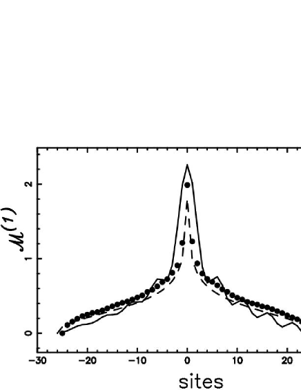
Figure 1: Graphs of ${\mathcal{M}}^{(1)}$, in case of absorbing boundaries: points denote the Monte Carlo simulation, the dashed line the numerical method via eqs. 10 and 1, and the full line the analytical solution (see 14). The parameters are $\alpha=0.8$, $L=51$; The Monte Carlo simulation comprises $10000$ trials, in Eq. (1) $n=2000$, and the index $m$ in Eq. (14) ranges from $1$ to $20$

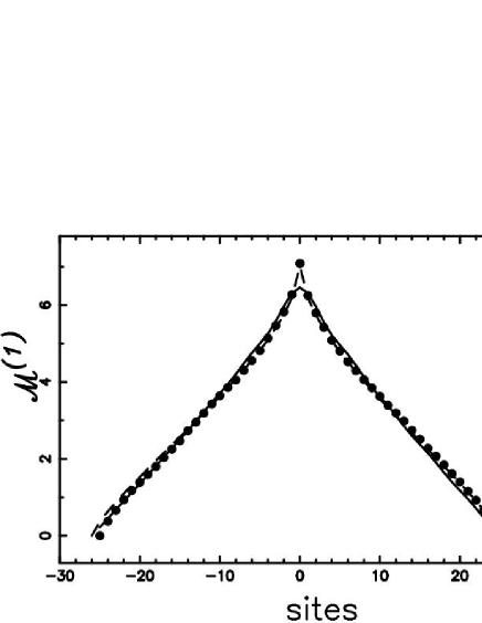
Figure 2: The same as Fig. 1 but $\alpha$=1.8

Figures (1) and (2) show ${\mathcal{M}}^{(1)}$ for $\alpha=0.8$ and $\alpha=1.8$ respectively. It can be seen that the graph of ${\mathcal{M}}$ tends to a triangular shape as $\alpha$ increases; indeed for simple symmetric random walk, ($\alpha=\infty$, $p(x)=1/2\delta_{|x|,1}$) ${\mathcal{M}}^{(1)}(x)=a-|x|$ bib:fzpha .

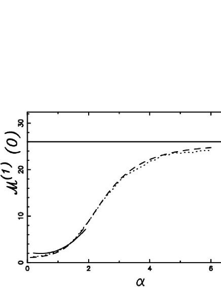
Figure 3: Graphs of ${\mathcal{M}}^{(1)}(0)$, as a function of $\alpha$, starting from $\alpha=0.2$, in case of absorbing boundaries. Points represent the Monte Carlo simulation, the dashed line the numerical solution of 10 and 1, and the continuous line results from Eq. (14), with $\alpha<2$. The horizontal line is the result for $\alpha=\infty$

Figure (3) presents the graph of ${\mathcal{M}}^{(1)}(0)$ as a function of $\alpha$; note that the inflection point of the curve occurs at $\alpha=2$, that is at the boundary between Levy flights and classical random walks. In other words, ${\mathcal{M}}^{(1)}(0)$ shows a “phase transition” from Levy flights, characterised by small number of visits, to the Gaussian regime where visits are more frequent.

IV Conclusion

The results of this note clarify how the mean number of times a site is visited by a random flyer depends on the dimensionality of the lattice, the value of $\alpha$ and the boundary conditions. In particular, it has been shown that unrestricted Levy flights are always transient, but for the unidimensional case with $\alpha\geq 1$; restricted flights are transient if the boundaries are absorbing. In the last case computations show that the direct numerical method agrees very closely with “experimental data” generated by the Monte Carlo simulation, whereas the agreement is worse for Eq. (14), especially when $\alpha$ is small (see Figs. 1 and 3); this is not surprising, since Eq. (10) deals directly with discrete variables, whereas Eq. (14) results from the diffusion approximation. On the other hand, obviously, Eq. (14) provides a more general, analytical formula for $\mathcal{M}^{(1)}$ and not just a set numerical values.

We thank the two anonymous referees for useful advice and criticism.

References

- (1) B.V. Gnedenko and A.N. Kolmogorov, Limit distributions for sums of independent random variables (Addison-Wesley Reading Mass, 1954)
- (2) J.P. Bouchaud and A. Georges, Physics Reports 195, 128 (1990).
- (3) J.E. Gilles and G.H. Weiss, Journal of Mathematical Physics. 11, 1307 (1970).
- (4) G. Berkolaiko and S. Havlin. Phys. Rev. E, 55, 1395 (1997)
- (5) M. Ferraro and L. Zaninetti, Phys. Rev. E, 64, 056107 (2001)
- (6) W. Feller, An Introduction to Probability Theory and Its Applications, Vol. I and II (John Wiley and Sons, New York, 1966)
- (7) A.V. Chechkin, V. Yu. Goncar, J. Klafter, R. Metzler, and L. V. Tanatarov, Journal of Statistical Physics, 115, 1505 (2004)
- (8) G.M. Viswanathan, V. Afanasyev , S. V. Buldyrev, S. Havlin, M.G.E. da Luz , E.P. Raposo and H. E. Stanley, Physica A 282, 1 (2000)
- (9) G. Boccignone and M. Ferraro, Physica A 331, 207 (2004)
- (10) M. Ferraro and L. Zaninetti, Physica A, 338, 307, (2004)
- (11) B. D. Hughes, M.F. Schlesinger and E. W. Montroll, Proc. Nat. Acad. Sci. USA, 6, 3287 (1981)
- (12) R. Metzler and J. Klafter, Physics Reports 339, 1 (2000)
- (13) E. V. Haynsworth and K. Golberg in Handbook of Mathematical Functions edited by M. I. Abramowitz and I. Stegun, (Dover Publication New York, 1965).
- (14) F.W.J. Olver Asymptotic and Special Functions (Academic Press, New York, 1974)
- (15) S.V. Buldyrev, S. Havlin, A. Ya. Kazazov, M.G.E. da Luz, E.P. Raposo, H.E. Stanley and G.M. Viswanathan, Phys. Rev. E 64, 041108 (2001).
- (16) G. H. Weiss, in Fractals in Science, edited by A. Bundle and S. Havlin (Springer-Verlag, New York, 1994).
- (17) M. Gitterman, Phys.Rev. E. 62, 6065 (2000)