Three methods for the description of the temporal response to a SH plane impulsive seismic wave in a soft elastic layer overlying a hard elastic substratum

Abstract

We treat the case of a flat stress-free surface (i.e., the ground in seismological applications) separating air from a homogeneous, isotropic, solid substratum overlain by a homogeneous, isotropic, solid layer (in contact with the ground) solicited by a SH plane body wave incident in the substratum. The analysis is first carried out in the frequency domain and subsequently in the time domain. The frequency domain response is normal in that no resonances are excited (a resonance is here understood to be a situation in which the response is infinite in the absence of dissipation). The translation of this in the time domain is that the scattered pulse is of relatively-short duration. The duration of the pulse is shown to be largely governed by radiation damping which shows up in the imaginary parts of the complex eigenfrequencies of the configuration. Three methods are elaborated for the computation of the time history and give rise to the same numerical solutions for a large variety of configurations of interest in the geophysical setting under the hypothesis of non-dissipative, dispersionless media. The method appealing to the complex eigenfrequency representation is shown to be the simplest and most physically-explicit way of obtaining the time history (under the same hypothesis). Moreover, it is particularly suited for the case in which modes can be excited as occurs when the incident wave is not plane or the boundary condition is not of the stress-free variety for all transverse coordinates on the ground plane.

1 Introduction

This work is inspired by the problem of predicting the effects of earthquakes in cities. It is known that the most dangerous effects are produced in cities built on soft underground underlain by a hard substratum. A simple model of the city is considered herein in which the buildings are absent (i.e., the ground is flat), the soft underground is constituted by a homogeneous, soft layer overlying, and in welded contact with, a homogeneous, hard substratum. This configuration is solicited by a SH plane body wave and the object is to determine the time history of response on the ground, preferably in a numerically-efficient, physically-understandable manner.

2 Space-time and space-frequency formulations

In the following, we shall be concerned with the determination of the vectorial displacement field $\mathbf{u}$ on, and underneath, the ground in response to a seismic solicitation. In general, $\mathbf{u}$ is a function of the spatial coordinates, incarnated in the vector $\mathbf{x}$ and time $t$, so that $\mathbf{u}=\mathbf{u}(\mathbf{x},t)$.

We first carry out our analysis in the frequency domain, and thus search for $\mathbf{u}(\mathbf{x},\omega)$, with $\omega$ the angular frequency.

Fourier analysis tells us that $\mathbf{u}(\mathbf{x},t)$ and $\mathbf{u}(\mathbf{x},\omega)$ are related by

$$\mathbf{u}(\mathbf{x},t)=\int_{-\infty}^{\infty}\mathbf{u}(\mathbf{x},\omega)\exp(-i\omega t)d\omega~{},$$ (1)

wherein it should be noted that $\mathbf{u}(\mathbf{x},\omega)$ is a generally-complex function, whereas $\mathbf{u}(\mathbf{x},t)$ is a real function. The second step will therefore deal with the computation of the integral in (1).

3 Frequency domain analysis of the reflection of a SH plane body wave from a stress-free planar boundary overlying a soft layer underlain by a hard substratum

3.1 Features of the problem

Since everything is invariant with $x_{3}$, the analysis takes place in the $x_{1}-x_{2}$ (sagittal) plane depicted in fig. 1.

In this figure: $\Gamma_{0}$ designates the (trace of the) interface between the substratum (half-space domain $\Omega_{0}$) and the soft layer (laterally-unbounded domain $\Omega_{1}$), and $\Gamma_{1}$ designates the (trace of the) flat ground. The medium $M^{2}$ above the latter is air, assumed to be the vacumn for the purpose of the analysis. The media in the layer and substratum are the elastic (or viscoelastic) solids $M^{1}$ and $M^{0}$ respectively.

The incident plane wave propagates in $\Omega_{0}$ toward the the interface $\Gamma_{0}$ and the ground $\Gamma_{1}$. Since the latter is stress-free (i.e., the normal and tangential components of traction are nil on the boundary), the total displacement field vanishes in the region $\Omega_{2}$ above the boundary (see fig. 1).

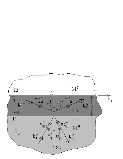
Figure 1: Cross section view of the configuration of a stress-free flat surface overlying a soft layer underlain by a hard solid substratum submitted to a SH plane wave, propagating initially in the substratum.

One can always choose the cartesian coordinate system so that the wavevector associated with the incident shear wave (the subscript $T$ will constitute a reminder that we deal with shear=transverse waves in the following) lies in the $x_{1}-x_{2}$ plane. This is assumed herein and signifies that the displacement associated with this wave is perpendicular to the $x_{1}-x_{2}$ plane and therefore lies in a horizontal plane. Thus, the incident wave is a shear wave and the associated displacement is horizontal; i.e., a shear-horizontal (SH) wave. Moreover, the motion associated with this wave is, due to the choice of the cartesian reference system, independent of the coordinate $x_{3}$. This implies that the resultant total motion induced by this incident wave is independent of $x_{3}$, i.e., the boundary value problem is 2D, so that it is sufficient to look for the displacement field in the $x_{1}-x_{2}$ plane. Actually, since we already know that the total displacement vanishes in the half plane above the boundary we must look for the total displacement field (hereafter designated by $\mathbf{u}^{0}(\mathbf{x},\omega)$) only in $\Omega_{0}$ and $\Omega_{1}$.

Hereafter, we designate the density and Lamé parameters in $\Omega_{j}$ by $\rho^{j}$ and $\lambda^{j},~{}\mu^{j}$ (for $j=0,1$) respectively.

3.2 Governing equations

The mathematical translation of the boundary value problem in the space-frequency domain is:

$$\mu u^{l}_{j,\beta\beta}(\mathbf{x},\omega)+(\lambda^{l}+\mu^{l})u^{l}_{\beta,\beta j}(\mathbf{x},\omega)+\rho^{l}\omega^{2}u^{l}_{j}(\mathbf{x},\omega)=0~{};~{}\forall\mathbf{x}=(x_{1},x_{2})\in\Omega_{l}~{}~{};\\ ~{}~{}j=1,2,3~{}~{},~{}~{}l=0,1~{}~{},~{}~{}\beta=1,2~{},$$ (2)

$$u^{l}_{j,3}(\mathbf{x},\omega)=0~{};~{}\forall\mathbf{x}\in\Omega_{l}~{}~{};~{}~{}j=1,2,3~{}~{},~{}~{}l=0,1~{},$$ (3)

$$(\lambda^{1}+2\mu^{1})u_{2,2}^{1}(\mathbf{x},\omega)+\lambda^{1}u_{1,1}^{1}(\mathbf{x},\omega)=0~{}~{}\text{on}~{}\Gamma_{1}~{},$$ (4)

$$\mu^{1}u_{3,2}^{1}(\mathbf{x},\omega)=~{}~{}\text{on}~{}\Gamma_{1}~{},$$ (5)

$$-\mu^{1}(u_{1,2}^{1}(\mathbf{x},\omega)+u_{2,1}^{1}(\mathbf{x},\omega))=0~{}~{}\text{on}~{}\Gamma_{1}~{}.$$ (6)

$$u_{2}^{0}(\mathbf{x},\omega)=u_{2}^{1}(\mathbf{x},\omega)~{}~{}\text{on}~{}\Gamma_{0}~{},$$ (7)

$$u_{3}^{0}(\mathbf{x},\omega)=u_{3}^{1}(\mathbf{x},\omega)~{}~{}\text{on}~{}\Gamma_{0}~{},$$ (8)

$$-u_{1}^{0}(\mathbf{x},\omega)=-u_{1}^{1}(\mathbf{x},\omega)~{}~{}\text{on}~{}\Gamma_{0}~{},$$ (9)

$$(\lambda^{0}+2\mu^{0})u_{2,2}^{0}(\mathbf{x},\omega)+\lambda^{0}u_{1,1}^{0}(\mathbf{x},\omega)=(\lambda^{1}+2\mu^{1})u_{2,2}^{1}(\mathbf{x},\omega)+\lambda^{1}u_{1,1}^{1}(\mathbf{x},\omega)~{}~{}\text{on}~{}\Gamma_{0}~{},$$ (10)

$$\mu^{0}u_{3,2}^{0}(\mathbf{x},\omega)=\mu^{1}u_{3,2}^{0}(\mathbf{x},\omega)~{}~{}\text{on}~{}\Gamma_{0}~{},$$ (11)

$$-\mu^{0}(u_{1,2}^{0}(\mathbf{x},\omega)+u_{2,1}^{0}(\mathbf{x},\omega))=-\mu^{1}(u_{1,2}^{1}(\mathbf{x},\omega)+u_{2,1}^{1}(\mathbf{x},\omega))~{}~{}\text{on}~{}\Gamma_{0}~{}.$$ (12)

$$u_{j}^{ld}(\mathbf{x},\omega):=u_{j}^{l}(\mathbf{x},\omega)-\delta_{l0}u_{0}^{i}(\mathbf{x},\omega)\sim\text{outgoing waves}~{};\\ ~{}\|\mathbf{x}\|\rightarrow\infty~{},~{}~{}\mathbf{x}\in\Omega_{j}~{},~{}j=0,1~{},~{}l=0,1~{},$$ (13)

wherein $u_{j}^{ld}(\mathbf{x},\omega)$ is the (unknown) diffracted field in $\Omega_{l}$, $\delta_{jk}$ the Kronecker delta symbol, and:

$$u^{i}_{3}(\mathbf{x},\omega)=A^{i-}_{3}\exp(i\mathbf{k}^{i-}_{T}\cdot\mathbf{x})~{},~{}~{}u^{i}_{1}(\mathbf{x},\omega)~{}=~{}u^{i}_{2}(\mathbf{x},\omega)=0~{};~{}\forall\mathbf{x}\in\Omega_{0}~{},$$ (14)

$$\mathbf{k}^{i-}_{T}=(k^{i}_{T1},~{}k^{i-}_{T2})~{},~{}k^{i}_{T1}=k^{0}_{T}\sin\theta_{T}^{i}~{},~{}k^{i-}_{T2}=-k^{0}_{T}\cos\theta_{T}^{i}~{},~{}k^{0}_{T}=\frac{\omega}{\sqrt{\frac{\mu^{0}}{\rho^{0}}}}~{},$$ (15)

$\theta_{T}^{i}$ being the angle of incidence with respect to the $x_{2}$ axis.

Eq. (2) is the space-frequency domain equation(s) of motion, (4)-(12) the boundary condition(s), (13) the radiation condition, and (14)-(15) the description of the incident wave.

Until further notice, we drop the $\omega-$dependence on all field quantities and consider it to be implicit.

3.2.1 Field representations incorporating the radiation condition

As in the previous section, and on account of the outgoing wave condition(s) (13), we adopt the following field representations:

$$u_{1}^{0d}=i\int_{-\infty}^{\infty}[\Phi^{0+}(k_{1})k_{1}\exp(i\mathbf{k}^{0+}_{L}\cdot\mathbf{x})+\Psi_{3}^{0+}(k_{1})k_{T2}^{0+}\exp(i\mathbf{k}^{0+}_{T}\cdot\mathbf{x})]dk_{1}~{},$$ (16)

$$u_{2}^{0d}=i\int_{-\infty}^{\infty}[\Phi^{0+}(k_{1})k_{L2}^{0+}\exp(i\mathbf{k}^{0+}_{L}\cdot\mathbf{x})-\Psi_{3}^{0+}(k_{1})k_{1}\exp(i\mathbf{k}^{0+}_{T}\cdot\mathbf{x})]dk_{1}~{},$$ (17)

$$u_{3}^{0d}=\int_{-\infty}^{\infty}\Xi_{3}^{0+}(k_{1})\exp(i\mathbf{k}^{0+}_{T}\cdot\mathbf{x})dk_{1}~{},$$ (18)

$$u_{1}^{1}=u_{1}^{1d}=i\int_{-\infty}^{\infty}\big{[}\Phi^{1-}(k_{1})k_{1}\exp(i\mathbf{k}^{1-}_{L}\cdot\mathbf{x})+\Psi_{3}^{1-}(k_{1})k_{T2}^{1-}\exp(i\mathbf{k}^{1-}_{T}\cdot\mathbf{x})+\\ \Phi^{1+}(k_{1})k_{1}\exp(i\mathbf{k}^{1+}_{L}\cdot\mathbf{x})+\Psi_{3}^{1+}(k_{1})k_{T2}^{1+}\exp(i\mathbf{k}^{1+}_{T}\cdot\mathbf{x})\big{]}dk_{1}~{},$$ (19)

$$u_{2}^{1}=u_{2}^{1d}=i\int_{-\infty}^{\infty}\big{[}\Phi^{1-}(k_{1})k_{L2}^{1-}\exp(i\mathbf{k}^{1-}_{L}\cdot\mathbf{x})-\Psi_{3}^{1-}(k_{1})k_{1}\exp(i\mathbf{k}^{1-}_{T}\cdot\mathbf{x})+\\ \Phi^{1+}(k_{1})k_{L2}^{1+}\exp(i\mathbf{k}^{1+}_{L}\cdot\mathbf{x})-\Psi_{3}^{1+}(k_{1})k_{1}\exp(i\mathbf{k}^{1+}_{T}\cdot\mathbf{x})\big{]}dk_{1}~{},$$ (20)

$$u_{3}^{1}=u_{3}^{1d}=\int_{-\infty}^{\infty}\big{[}\Xi_{3}^{1-}(k_{1})\exp(i\mathbf{k}^{1-}_{T}\cdot\mathbf{x})+\Xi_{3}^{1+}(k_{1})\exp(i\mathbf{k}^{1+}_{T}\cdot\mathbf{x})\big{]}dk_{1}~{},$$ (21)

wherein

$$\mathbf{k}^{j\pm}_{L}=(k_{1},k^{j\pm}_{L2})~{}~{},~{}~{}k^{j\pm}_{L2}=\pm\sqrt{\left(k_{L}^{j}\right)^{2}-\left(k_{1}\right)^{2}}~{}~{},~{}~{}\Re\sqrt{\left(k_{L}^{j}\right)^{2}-\left(k_{1}\right)^{2}}\geq 0~{},~{}\Im\sqrt{\left(k_{L}^{j}\right)^{2}-\left(k_{1}\right)^{2}}\geq 0~{},$$ (22)

$$\mathbf{k}^{j\pm}_{T}=(k_{1},k^{j\pm}_{T2})~{}~{},~{}~{}k^{j\pm}_{T2}=\pm\sqrt{\left(k_{T}^{j}\right)^{2}-\left(k_{1}\right)^{2}}~{}~{},~{}~{}\Re\sqrt{\left(k_{T}^{j}\right)^{2}-\left(k_{1}\right)^{2}}\geq 0~{},~{}\Im\sqrt{\left(k_{T}^{j}\right)^{2}-\left(k_{1}\right)^{2}}\geq 0~{},$$ (23)

with

$$k^{j}_{L}=\frac{\omega}{c^{j}_{L}}=\frac{\omega}{\sqrt{\frac{\lambda^{j}+2\mu^{j}}{\rho^{j}}}}~{}~{},~{}~{}k^{j}_{T}=\frac{\omega}{c^{j}_{T}}=\frac{\omega}{\sqrt{\frac{\mu^{j}}{\rho^{j}}}}~{}.$$ (24)

Note that these field representations involve nine unknown functions $\Phi^{0+},~{}\Psi^{0+},~{}\Xi^{0+}$, $\Phi^{1-},~{}\Psi^{1-},~{}\Xi^{1-}$, $\Phi^{1+},~{}\Psi^{1+},~{}\Xi^{1+}$. The latter will be obtained by applying the nine boundary conditions embodied in (4)-(12).

3.3 Application of the boundary condition(s)

The use of (4), (6), (7), (9), (10), and (12), in (16)-(24) gives rise to:

$$\Phi^{0+}=\Psi_{3}^{0+}=\Phi^{1-}=\Psi_{3}^{1-}=\Phi^{1+}=\Psi_{3}^{1+}=0~{}~{};~{}~{}\forall k_{1}\in\mathbb{R}~{}.$$ (25)

The next step consists in using (5) in (21) to obtain:

$$i\mu^{1}\int_{-\infty}^{\infty}\big{[}k_{2}^{1-}\Xi_{3}^{1-}(k_{1})+k_{2}^{1+}\Xi_{3}^{1+}(k_{1})\big{]}\exp(ik_{1}x_{1})dk_{1}=0~{}~{};\forall x_{1}\in\mathbb{R}~{}.$$ (26)

By Fourier inversion we get

$$\Xi_{3}^{1-}=\Xi_{3}^{1+}:=A^{1}~{}~{};\forall k_{1}\in\mathbb{R}~{},$$ (27)

whence

$$u^{1}(\mathbf{x})=2\int_{-\infty}^{\infty}A^{1}(k_{1})\cos(k_{2}^{1}x_{2})\exp(ik_{1}x_{1})dk_{1}=~{}~{};\forall\mathbf{x}\in\Omega_{1}~{},$$ (28)

wherein

$$k_{2}^{j}:=k_{T2}^{j+}~{}~{};~{}~{}j=0,1~{}~{},~{}~{}k_{2}^{i}:=k_{T2}^{i+}=-k_{2}^{i-}~{}.$$ (29)

By the same token, we can write (21) as

$$u^{0d}(\mathbf{x})=\int_{-\infty}^{\infty}A^{0+}(k_{1})\exp(ik_{2}^{0+}x_{2})\exp(ik_{1}x_{1})dk_{1}=~{}~{};\forall\mathbf{x}\in\Omega_{0}~{},$$ (30)

so that using (28) and (30) together with (8) and (11) leads to:

$$A^{i-}\exp(-ik_{2}^{i}h)\exp(ik^{i}x_{1})+\int_{-\infty}^{\infty}A^{0+}(k_{1})\exp(ik_{2}^{0}h)\exp(ik_{1}x_{1})dk_{1}-\\ \int_{-\infty}^{\infty}2A^{1}(k_{1})\cos(k_{2}^{1}h)\exp(ik_{1}x_{1})dk_{1}=0~{}~{};\forall x_{1}\in\mathbb{R}~{},$$ (31)

$$-i\mu^{0}k_{2}^{i}A^{i-}\exp(-ik_{2}^{i}h)\exp(ik^{i}x_{1})+\int_{-\infty}^{\infty}i\mu^{0}k_{2}^{0}A^{0+}(k_{1})\exp(ik_{2}^{0}h)\exp(ik_{1}x_{1})dk_{1}+\\ \int_{-\infty}^{\infty}\mu^{1}k_{2}^{1}2A^{1}(k_{1})\sin(k_{2}^{1}h)\exp(ik_{1}x_{1})dk_{1}=0~{}~{};\forall x_{1}\in\mathbb{R}~{}.$$ (32)

By Fourier inversion we find:

$$A^{i-}\exp(-ik_{2}^{i}h)\delta(k_{1}-k_{1}^{i})+A^{0+}(k_{1})\exp(ik_{2}^{0}h)-2A^{1}(k_{1})\cos(k_{2}^{1}h)=0~{}~{};\forall k_{1}\in\mathbb{R}~{},$$ (33)

$$-i\mu^{0}k_{2}^{i}A^{i-}\exp(-ik_{2}^{i}h)\delta(k_{1}-k_{1}^{i})+i\mu^{0}k_{2}^{0}A^{0+}(k_{1})\exp(ik_{2}^{0}h)+\mu^{1}k_{2}^{1}2A^{1}(k_{1})\sin(k_{2}^{1}h)=0~{}~{};\forall x_{1}\in\mathbb{R}~{}.$$ (34)

This system of two equations can be written as the matrix equation

$$\begin{pmatrix}\exp(ik_{2}^{0}h)&-\cos(k_{2}^{1}h)\\ i\mu^{0}k_{2}^{0}\exp(ik_{2}^{0}h)&\mu^{1}k_{2}^{1}\sin(k_{2}^{1}h)\end{pmatrix}\begin{pmatrix}A^{0+}\\ 2A^{1}\end{pmatrix}=\begin{pmatrix}-A^{i-}\exp(-ik_{2}^{i}h)\delta(k_{1}-k_{1}^{i})\\ i\mu^{0}k_{2}^{i}A^{i-}\exp(-ik_{2}^{i}h)\delta(k_{1}-k_{1}^{i})\end{pmatrix}~{}.$$ (35)

It follows that:

$$A^{0+}(k_{1})=\mathcal{R}^{0}(k_{1})A^{i-}\delta(k_{1}-k_{1}^{i})~{},$$ (36)

wherein

$$\mathcal{R}^{0}(k_{1})=\left[\frac{\mu^{0}k_{2}^{i}\cos(k_{2}^{1}h)+i\mu^{1}k_{2}^{1}\sin(k_{2}^{1}h)}{\mu^{0}k_{2}^{i}\cos(k_{2}^{1}h)-i\mu^{1}k_{2}^{1}\sin(k_{2}^{1}h)}\right]\exp[-i(k_{2}^{i}+k_{2}^{0})h]~{},$$ (37)

and

$$A^{1}(k_{1})=\frac{1}{2}\mathcal{R}^{1}(k_{1})A^{i-}\delta(k_{1}-k_{1}^{i})~{},$$ (38)

wherein

$$\mathcal{R}^{1}(k_{1})=\left[\frac{\mu^{0}k_{2}^{0}+\mu^{0}k_{2}^{i}}{\mu^{0}k_{2}^{i}\cos(k_{2}^{1}h)-i\mu^{1}k_{2}^{1}\sin(k_{2}^{1}h)}\right]\exp(-ik_{2}^{i}h)~{}.$$ (39)

3.4 The scattered field

The consequence of all this is that:

$$u_{1}^{0d}(\mathbf{x},\omega)=u_{2}^{0d}(\mathbf{x},\omega)=0~{}~{};~{}~{}\forall\mathbf{x}\in\Omega_{0}~{},$$ (40)

$$u_{3}^{0d}(\mathbf{x},\omega)=\int_{-\infty}^{\infty}A^{0+}e^{i(k_{1}x_{1}+k_{2}^{0}x_{2})}dk_{1}=\mathcal{R}^{0}(k_{1}^{i})A^{i-}e^{i(k_{1}^{i}x_{1}+k_{2}^{0i}x_{2})}~{}~{};~{}~{}\forall\mathbf{x}\in\Omega_{0}~{},$$ (41)

$$u_{1}^{1}(\mathbf{x},\omega)=u_{1}^{1d}(\mathbf{x},\omega)=u_{2}^{1d}(\mathbf{x},\omega)=u_{2}^{1}(\mathbf{x},\omega)=0~{}~{},;~{}~{}\forall\mathbf{x}\in\Omega_{1}~{},$$ (42)

$$u_{3}^{1}(\mathbf{x},\omega)=u_{3}^{1d}(\mathbf{x},\omega)=2\int_{-\infty}^{\infty}A^{1}e^{ik_{1}x_{1}}\cos(k_{2}^{0}x_{2})dk_{1}=\mathcal{R}^{1}(k_{1}^{i})A^{i-}e^{ik_{1}^{i}x_{1}}\cos(k_{2}^{1i}x_{2})~{}~{};~{}~{}\forall\mathbf{x}\in\Omega_{1}~{},$$ (43)

wherein

$$k_{2}^{ji}:=\sqrt{(k^{j})^{2}-(k_{1}^{i})^{2}}=\sqrt{(k^{j})^{2}-(k^{0}\sin\theta_{T}^{i})^{2}}~{}~{},~{}~{}\Re k_{2}^{ji}\geq 0~{},~{}~{}\Im k_{2}^{ji}\geq 0~{}~{},~{}~{}j=0,1~{}~{}(k_{2}^{0i}=k_{2}^{i})~{},$$ (44)

$$\mathcal{R}^{0}(k_{1}^{i})=\left[\frac{\mu^{0}k_{2}^{0i}\cos(k_{2}^{1i}h)+i\mu^{1}k_{2}^{1}\sin(k_{2}^{1i}h)}{\mu^{0}k_{2}^{0i}\cos(k_{2}^{1i}h)-i\mu^{1}k_{2}^{1i}\sin(k_{2}^{1i}h)}\right]\exp[-2ik_{2}^{0i}h]~{},$$ (45)

and

$$\mathcal{R}^{1}(k_{1}^{i})=\left[\frac{2\mu^{0}k_{2}^{0i}}{\mu^{0}k_{2}^{0i}\cos(k_{2}^{1i}h)-i\mu^{1}k_{2}^{1i}\sin(k_{2}^{1i}h)}\right]\exp[-ik_{2}^{0i}h]~{}.$$ (46)

These results, together with (14), indicate that the diffracted fields in $\Omega_{0}$ and $\Omega_{1}$ have the same (SH) polarization ($\boldsymbol{\pi}$ in fig. 1) as the incident field.

3.5 Total fields in the two media

The preceding results show that the fields in the two media can be decomposed as follows:

$$u_{3}^{0}(\mathbf{x},\omega)=u_{3}^{0-}(\mathbf{x},\omega)+u_{3}^{0+}(\mathbf{x},\omega)~{}~{};\forall\mathbf{x}\in\Omega_{0}~{},$$ (47)

wherein

$$u_{3}^{0-}(\mathbf{x},\omega)=u_{3}^{i}(\mathbf{x},\omega)=A^{i-}e^{i[k_{1}^{i}x_{1}-k_{2}^{0i}x_{2}]}~{},$$ (48)

$$u_{3}^{0+}(\mathbf{x},\omega)=\mathcal{R}^{0}(k_{1}^{i})A^{i-}e^{i[k_{1}^{i}x_{1}+k_{2}^{0i}x_{2}]}~{},$$ (49)

and

$$u_{3}^{1}(\mathbf{x},\omega)=u_{3}^{1-}(\mathbf{x},\omega)+u_{3}^{1+}(\mathbf{x},\omega)~{}~{};\forall\mathbf{x}\in\Omega_{1}~{}$$ (50)

wherein

$$u_{3}^{1-}(\mathbf{x},\omega):=\frac{\mathcal{R}^{1}(k_{1}^{i})}{2}A^{i-}e^{i[k_{1}^{i}x_{1}-k_{2}^{1i}x_{2}]}~{},$$ (51)

$$u_{3}^{1+}(\mathbf{x},\omega):=\frac{\mathcal{R}^{1}(k_{1}^{i})}{2}A^{i-}e^{i[k_{1}^{i}x_{1}+k_{2}^{1i}x_{2}]}~{}.$$ (52)

Remark
These results indicate that the diffracted field in $\Omega_{0}$ reduces to a specularly-reflected wave $u_{3}^{0+}$ and the diffracted (as well as total) field in $\Omega_{1}$ reduces to a sum of a refracted-reflected wave $u_{3}^{1+}$ and a refracted-transmitted wave $u_{3}^{1-}$.

Remark
$u_{3}^{0-}$ and $u_{3}^{0+}$ are plane homogeneous (body) waves so that the field in the half-space underneath the layer is composed of two body waves.

Remark
Since we consider only the case of geological interest in which the substratum is harder than the layer, the S-wave phase velocity in the substratum is larger than the S-wave phase velocity in the layer, which means that $k^{0}<k^{1}$ and consequently $k_{2}^{1i}$ is real, so that both $u_{3}^{1-}$ and $u_{3}^{1+}$ are body waves. Thus, the field in the layer is also composed of two body waves.

Remark
An important corollary of the previous remarks is (in the case of geological interest) that an incident (plane) body wave in the substratum can only excite (plane) body waves in both the substratum and the layer. Thus, if we want a surface wave to be excited somewhere underneath the ground, then we have to introduce some sort of modification of either the excitation, the nature of the media, or the nature of the boundary condition on the ground.

3.6 Numerical results for the frequency domain response in the layer

Recall that the frequency domain displacement response in the layer is of the form

$$u_{3}^{1}(\mathbf{x},\omega)=u_{3}^{1-}(\mathbf{x},\omega)+u_{3}^{1+}(\mathbf{x},\omega)~{}.$$ (53)

with

$$u_{3}^{1\pm}(\mathbf{x},\omega)=\frac{\mathcal{R}^{1}(k_{1}^{i})}{2}A^{i-}(\omega)e^{i[k_{1}^{i}x_{1}\pm k_{2}^{1i}x_{2}]}~{},$$ (54)

so that one half of the total frequency domain displacement response on the ground at point $\mathbf{x}=(0,0)$ is given by

$$\frac{u_{3}^{1}(0,0,\omega)}{2}=u_{3}^{1\pm}(0,0,\omega)=\frac{\mathcal{R}^{1}(k_{1}^{i})}{2}A^{i-}(\omega)~{},$$ (55)

wherein:

$$\frac{\mathcal{R}^{1}(k_{1}^{i})}{2}=\frac{i}{D(k_{1}^{i})}~{},$$ (56)

$$D(k_{1}^{i})=ia\cos(\gamma\omega)+b\sin(\gamma\omega)~{},$$ (57)

$$a=1~{}~{},~{}~{}b=b(\omega,s^{i})=\frac{\mu^{1}(\omega)\kappa^{1i}(\omega,s^{i})}{\mu^{0}\kappa^{0i}(s^{i})}~{}~{},~{}~{}\gamma(\omega,s^{i})=\kappa^{1i}(\omega,s^{i})\frac{h}{c_{T}^{0}}~{},$$ (58)

$$\kappa^{ji}:=\frac{k_{2}^{ji}}{k^{0}}=\sqrt{[c_{T}^{0}/c_{T}^{j}(\omega)]^{2}-(s^{i})^{2}}~{}.$$ (59)

In the five figures 2, 3, 4, 5, 6 we plot the spectrum ( $A^{i-}(\omega)$) of a Ricker pulse excitation, the transfer function $\frac{u_{3}^{1}(0,0,\omega)}{2A^{i}(\omega)}$, and the spectrum of the displacement response $\frac{u_{3}^{1}(0,0,\omega)}{2}$.

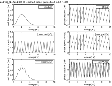
Figure 2: Spectrum of displacement response at $\mathbf{x}=(0,0)$. $\mathcal{A}=1$, $\alpha=1$, $\beta=4$, $\gamma=4$, $a=1$, $b=0.7$, corresponding to a case of separated pulses. The left-hand curves pertain to moduli, and the right hand curves to phases of the spectra.

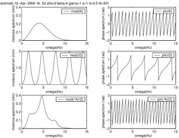
Figure 3: Spectrum of displacement response at $\mathbf{x}=(0,0)$. $\mathcal{A}=1$, $\alpha=2$, $\beta=4$, $\gamma=1$, $a=1$, $b=0.5$, corresponding to a case of merged pulses. The left-hand curves pertain to moduli, and the right hand curves to phases of the spectra.

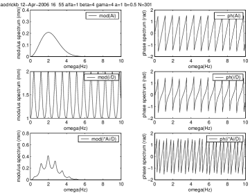
Figure 4: Spectrum of displacement response at $\mathbf{x}=(0,0)$. $\mathcal{A}=1$, $\alpha=1$, $\beta=4$, $\gamma=4$, $a=1$, $b=0.5$, corresponding to a case of separated pulses. The left-hand curves pertain to moduli, and the right hand curves to phases of the spectra.

Figure 5: Spectrum of displacement response at $\mathbf{x}=(0,0)$. $\mathcal{A}=1$, $\alpha=2$, $\beta=4$, $\gamma=1$, $a=1$, $b=0.1$, corresponding to a case of merged pulses. The left-hand curves pertain to moduli, and the right hand curves to phases of the spectra.

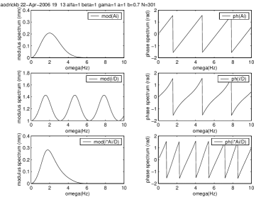
Figure 6: Spectrum of displacement response at $\mathbf{x}=(0,0)$. $\mathcal{A}=1$, $\alpha=1$, $\beta=1$, $\gamma=1$, $a=1$, $b=0.7$, corresponding to a case of a so-called ”anomalous” pulse. The left-hand curves pertain to moduli, and the right hand curves to phases of the spectra.

We note that the spectrum of displacement response contains spikes that are all the sharper and more intense the larger is the contrast between $a$ and $b$. As will be shown further on, these sharper spikes lead to larger-duration response in the time domain.

4 Time domain analysis of the reflection of a SH plane body wave from a stress-free planar boundary overlying a soft layer underlain by a hard substratum

4.1 Obtention of the time domain response from the frequency domain response

We had

$$u_{3}^{j}(\mathbf{x},t)=\int_{-\infty}^{\infty}u_{3}^{j}(\mathbf{x},\omega)\exp(-i\omega t)d\omega~{}~{};~{}~{}j=0,1~{},$$ (60)

and due to the fact that $u_{3}^{j}(\mathbf{x},t)$ is a real function, we must have

$$[u_{3}^{j}(\mathbf{x},\omega)]^{*}=u_{3}^{j}(\mathbf{x},-\omega)~{},$$ (61)

(wherein the symbol $*$ designates the complex conjugate operator) from which it follows that

$$u_{3}^{j}(\mathbf{x},t)=2\Re\int_{0}^{\infty}u_{3}^{j}(\mathbf{x},\omega)\exp(-i\omega t)d\omega~{}.$$ (62)

We shall employ (62) or (60) to obtain the temporal response from the frequency response function $u_{3}^{j}(\mathbf{x},\omega)$. More precisely, we shall be concerned with the evaluation of

$$u_{3}^{j\pm}(\mathbf{x},t)=\int_{-\infty}^{\infty}\left[u_{3}^{j-}(\mathbf{x},\omega)+u_{3}^{j+}(\mathbf{x},\omega)\right]\exp(-i\omega t)d\omega~{}~{};~{}~{}j=0,1~{}.$$ (63)

4.2 The frequency content and time history of a of a plane transient body wave

For a so-called upward-propagating SH-plane wave, we have

$$u_{1}^{i}(\mathbf{x},\omega)=0~{},~{}~{}u_{2}^{i}(\mathbf{x},\omega)=0~{},~{}~{}u_{3}^{i}(\mathbf{x},\omega)=A^{i-}(\omega)\exp(i\mathbf{k}_{T}^{i-}(\omega)\cdot\mathbf{x})~{}.$$ (64)

wherein

$$\mathbf{k}_{T}^{i-}=(k_{T1}^{i},k_{T2}^{i-})~{},~{}~{}k_{T1}^{i}:=k_{T}^{0}\sin\theta_{T}^{i}~{},~{}~{}k_{T2}^{i\pm}:=\pm k_{T}^{0}\cos\theta_{T}^{i}~{},~{}~{}k_{T}^{0}(\omega)=\frac{\omega}{c_{T}(\omega)}~{},$$ (65)

and $\theta_{T}^{i}$ is the incident angle measured clockwise from the $+x_{2}$ axis. In the above relations, $A^{i-}(\omega)$ is termed the frequency-domain amplitude or spectrum of the incident SH plane wave.

The time history of this incident wave is

$$\mathbf{u}^{i}(\mathbf{x},t)=\mathbf{u}^{0-}(\mathbf{x},t)=\int_{-\infty}^{\infty}\mathbf{u}^{0-}(\mathbf{x},\omega)\exp(-i\omega t)d\omega~{},$$ (66)

or

$$\mathbf{u}^{i}(\mathbf{x},t)=\mathbf{u}^{0-}(\mathbf{x},t)=2\Re\int_{0}^{\infty}\mathbf{u}^{0-}(\mathbf{x},\omega)\exp(-i\omega t)d\omega~{}.$$ (67)

4.2.1 Spectrum and time history of a Ricker pulse

The amplitude spectrum $A^{i-}(\omega)$ of a Ricker pulse (Sanchez-Sesma 1985) is given by

$$A^{i-}(\omega)=-\mathcal{A}\frac{1}{\sqrt{\pi}}\frac{\omega^{2}}{4\alpha^{3}}\exp\left(i\beta\omega-\frac{\omega^{2}}{4\alpha^{2}}\right)~{},$$ (68)

wherein $\mathcal{A}$, $\alpha$ and $\beta$ are real constants (i.e., independent of $\omega$). It follows that

$$[A^{i-}(\omega)]^{*}=-\mathcal{A}\frac{1}{\sqrt{\pi}}\frac{\omega^{2}}{4\alpha^{3}}\exp\left(-i\beta\omega-\frac{\omega^{2}}{4\alpha^{2}}\right)=A^{i-}(-\omega)~{},$$ (69)

so that the temporal history associated with this pulse is

$$A^{i-}(t)=\int_{-\infty}^{\infty}A^{i-}(\omega)\exp(-i\omega t)d\omega~{}.$$ (70)

More precisely:

$$A^{i-}(t)=\left(-\mathcal{A}\frac{1}{4\alpha^{3}\sqrt{\pi}}\right)\int_{-\infty}^{\infty}\omega^{2}\exp\left[i\omega(\beta-t)-\frac{\omega^{2}}{4\alpha^{2}}\right]d\omega=\\ \left(-\mathcal{A}\frac{1}{4\alpha^{3}\sqrt{\pi}}\right)\int_{-\infty}^{\infty}\omega^{2}\exp\left[-\frac{1}{4\alpha^{2}}\{\omega^{2}+4\alpha^{2}i\omega(t-\beta)\}\right]d\omega~{}.$$ (71)

But

$$\omega^{2}+4\alpha^{2}i\omega(t-\beta)=[\omega+i2\alpha^{2}(t-\beta)]^{2}+4\alpha^{4}(t-\beta)^{2}~{},$$ (72)

so that

$$A^{i-}(t)=\left(-\mathcal{A}\frac{1}{4\alpha^{3}\sqrt{\pi}}\right)\exp[-\alpha^{2}(t-\beta)^{2}]\int_{-\infty}^{\infty}\omega^{2}\exp\left[-\frac{\{\omega+i2\alpha^{2}(t-\beta)\}^{2}}{4\alpha^{2}}\right]d\omega~{},$$ (73)

which, after the change of variables

$$\varpi=\omega+i2\alpha^{2}(t-\beta)~{},$$ (74)

becomes

$$A^{i-}(t)=\left(-\mathcal{A}\frac{1}{4\alpha^{3}\sqrt{\pi}}\right)\exp[-\alpha^{2}(t-\beta)^{2}]\int_{-\infty}^{\infty}[\varpi-i2\alpha^{2}(t-\beta)]^{2}\exp\left[-\frac{\varpi^{2}}{4\alpha^{2}}\right]d\varpi:=\\ \left(-\mathcal{A}\frac{1}{4\alpha^{3}\sqrt{\pi}}\right)\left[J_{2}(t)-i4\alpha^{2}(t-\beta)J_{1}(t)-4\alpha^{4}(t-\beta)^{2}J_{0}(t)\right]~{},$$ (75)

wherein:

$$J_{0}(t)=\int_{-\infty}^{\infty}\exp\left[-\frac{\varpi^{2}}{4\alpha^{2}}\right]d\varpi=2\int_{0}^{\infty}\exp\left[-\frac{\varpi^{2}}{4\alpha^{2}}\right]d\varpi~{},$$ (76)

$$J_{1}(t)=\int_{-\infty}^{\infty}\varpi\exp\left[-\frac{\varpi^{2}}{4\alpha^{2}}\right]d\varpi=0~{},$$ (77)

$$J_{2}(t)=\int_{-\infty}^{\infty}\varpi^{2}\exp\left[-\frac{\varpi^{2}}{4\alpha^{2}}\right]d\varpi=2\int_{0}^{\infty}\varpi^{2}\exp\left[-\frac{\varpi^{2}}{4\alpha^{2}}\right]d\varpi~{}.$$ (78)

Employing the following identities (Hodgman 1957):

$$\int_{0}^{\infty}\exp\left(-\frac{\eta^{2}}{b^{2}}\right)d\eta=\frac{b\sqrt{\pi}}{2}~{},$$ (79)

$$\int_{0}^{\infty}\eta^{2}\exp\left(-\frac{\eta^{2}}{b^{2}}\right)d\eta=\frac{b^{3}\sqrt{\pi}}{4}~{},$$ (80)

we finally obtain

$$J_{0}(t)=2\alpha\sqrt{\pi}~{}~{},~{}~{}J_{2}(t)=4\alpha^{3}\sqrt{\pi}~{},$$ (81)

so that

$$A^{i-}(t)=\left(-\mathcal{A}\frac{1}{4\alpha^{3}\sqrt{\pi}}\right)\left[4\alpha^{3}\sqrt{\pi}-2\alpha\sqrt{\pi}4\alpha^{4}(t-\beta)^{2}\right]\exp[-\alpha^{2}(t-\beta)^{2}]~{},$$ (82)

or

$$A^{i-}(t)=\mathcal{A}\left[-1+2\alpha^{2}(t-\beta)^{2}\right]\exp[-\alpha^{2}(t-\beta)^{2}]~{}.$$ (83)

Remark
The maxima of $A^{i-}(t)/\mathcal{A}$ are obtained from $dA^{i-}(t)/dt=0$, i.e.,

$$2\alpha^{2}(t-\beta)\{2-[-1+2\alpha^{2}(t-\beta)^{2}]\}\exp[-\alpha^{2}(t-\beta)^{2}]=0~{}.$$ (84)

the solutions of which are

$$t_{0}=\beta~{}~{},~{}~{}t_{-}=\beta-\sqrt{\frac{3}{2\alpha^{2}}}~{}~{},~{}~{}t_{-}=\beta+\sqrt{\frac{3}{2\alpha^{2}}}~{}.$$ (85)

It follows that

$$A^{i-}(t_{0})/\mathcal{A}=-1~{}~{},~{}~{}A^{i-}(t_{\pm})/\mathcal{A}=2\exp\left(-\frac{3}{2}\right)=0.4463~{}.$$ (86)

Remark
Thus, The minimum of $A^{i-}(t)/\mathcal{A}$ is attained at $t=t_{0}=\beta$ and is equal to $A^{i-}(t_{0})/\mathcal{A}=-1$. This means that the minimum of $A^{i-}(t)/\mathcal{A}$ is independent of both $\alpha$ and $\beta$. Furthermore, $\beta$ is the instant at which the pulse attains its minimum, and this minimum is also the maximum of $\|A^{i-}(t)/\mathcal{A}\|$.

Remark
$A^{i-}(t)/\mathcal{A}=0$ when $-1+2\alpha^{2}(t-\beta)^{2}=0$, i.e., when $t=\beta\pm\frac{1}{2\alpha^{2}}$, so that $1/\alpha$ is an indicator of the width of the main lobe of the pulse, i.e., the larger is $\alpha$, the smaller is the width of the main lobe of the pulse.

Remark
The maxima of $A^{i-}(t)/\mathcal{A}$ are attained at $t=t_{-}$ and $t=t_{+}$, and their value (0.4463) is independent of both $\alpha$ and $\beta$.

Remark
The moduli of the spectra of the Ricker pulses for various values of $\alpha$ are depicted in fig. 7.

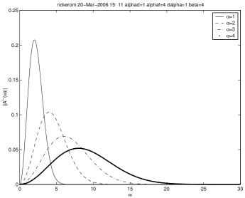
Figure 7: Modulus of the spectrum function $A^{i-}(\omega)$ versus $\omega$ for various values of $\alpha$. $\mathcal{A}=1$, $\beta=4$.

Note that these spectra do not depend on $\beta$. The latter only affects the phase of $A^{i-}(\omega)$.

Remark
The time history of the Ricker pulses for various values of $\alpha$ are depicted in fig. 8 for the fixed value $\beta=4$. This confirms the fact that the larger is $\alpha$, the narrower is the Ricker pulse.

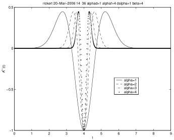
Figure 8: Time history $A^{i-}(t)$ versus $t$ for various values of $\alpha$. $\beta=4$ and $\mathcal{A}=1$.

Remark
Let $G(t)$ be the Gaussian function

$$G(t)=\frac{\mathcal{A}}{2\alpha^{2}}\exp[-\alpha^{2}(t-\beta)^{2}]~{}.$$ (87)

Then

$$\frac{dG(t)}{dt}=-\mathcal{A}(t-\beta)\exp[-\alpha^{2}(t-\beta)^{2}]~{},~{}\frac{d^{2}G(t)}{dt^{2}}=\mathcal{A}[-1+2\alpha^{2}(t-\beta)^{2}]\exp[-\alpha^{2}(t-\beta)^{2}]=A^{i-}(t)~{},$$ (88)

which shows that the Ricker pulse is identical to the second time derivative of the Gaussian pulse.

4.2.2 Spectrum and time history of a Ricker pulse plane body wave propagating in free space

The wave we are concerned with is actually what was heretofore termed the ”incident plane wave”. The plane body wave nature of the disturbance is embodied in the frequency domain function

$$u_{3}^{0-}(\mathbf{x},\omega)=A^{i-}(\omega)\exp[i(k_{1}^{i}x_{1}-k_{2}^{0i}x_{2})]=A^{i-}(\omega)\exp\left[i\omega\left(\frac{x_{1}}{c_{T}^{0}}s^{i}-\frac{x_{2}}{c_{T}^{0}}\kappa^{0i}\right)\right]~{},$$ (89)

wherein

$$s^{i}=\sin\theta_{T}^{i}~{}~{},~{}~{}\kappa^{0i}=\sqrt{1-(s^{i})^{2}}=\cos\theta_{T}^{i}~{}.$$ (90)

The Ricker pulse nature of the plane wave is embodied in the spectrum function

$$A^{i-}(\omega)=\left(-\mathcal{A}\frac{1}{\sqrt{\pi}}\frac{\omega^{2}}{4\alpha^{3}}\right)\exp\left(i\beta\omega-\frac{\omega^{2}}{4\alpha^{2}}\right)~{},$$ (91)

so that the time history of this wave is given by the Fourier transform

$$u_{3}^{i}(\mathbf{x},t)=\int_{-\infty}^{\infty}A^{i-}(\omega)\exp[-i\omega\tau(\mathbf{x},t,s^{i})]d\omega~{},$$ (92)

wherein

$$\tau(\mathbf{x},t,s^{i})=t-\frac{x_{1}}{c_{T}^{0}}s^{i}+\frac{x_{2}}{c_{T}^{0}}c^{i}~{}.$$ (93)

We assume that $M^{0}$ is non-dispersive, i.e., $\mu^{0}$ and $c_{T}^{0}$ do not depend on $\omega$, so that $\tau(\mathbf{x},t,s^{i})$ is independent of $\omega$. Then $u_{3}^{i}(\mathbf{x},t)$ is of the same form as $A^{i-}(t)$ (see (70)) if we replace therein $t$ by $\tau(\mathbf{x},t,s^{i})$, i.e.,

$$u_{3}^{i}(\mathbf{x},t)=A^{i-}(\tau(\mathbf{x}),t,s^{i})~{},$$ (94)

so that employing the previous result in (83):

$$u_{3}^{i}(\mathbf{x},t)=\mathcal{A}\left[-1+2\alpha^{2}\{\tau(\mathbf{x})-\beta\}^{2}\right]\exp[-\alpha^{2}\{\tau(\mathbf{x},t,s^{i})-\beta\}^{2}]~{}.$$ (95)

Remark
The same remarks apply to this time history as to $A^{i-}(t)$ except that $\tau(\mathbf{x},t,s^{i})$ replaces $t$. Thus, the Ricker pulse plane body wave attains its maximum (in absolute value) at $\tau(\mathbf{x},t,s^{i})=\beta$, and the main lobe of the pulse is all the narrower the larger is $\alpha$.

4.3 Time history of the reflected and transmitted plane body wave pulses in the basement and layer

4.3.1 Preliminaries

Recall that $k^{j}=\frac{\omega}{c_{T}^{j}}$. We encountered previously, in connection with the frequency domain response in $\Omega_{0}$ and $\Omega_{1}$, plane wave functions of the type

$$u_{3}^{j\pm}(\mathbf{x},\omega):=\mathcal{R}^{j}(s^{i},\omega)A^{i-}(\omega)\exp[i(k_{1}^{i}x_{1}\pm k_{2}^{ji}x_{2})]=\\ \mathcal{R}^{j}(s^{i},\omega)A^{i-}(\omega)\exp\left[i\omega\left(s^{i}\frac{x_{1}}{c_{T}^{0}}\pm\kappa^{ji}\frac{x_{2}}{c_{T}^{0}}\right)\right]~{}~{};~{}~{}j=0,1~{},$$ (96)

wherein (recall that we assumed that $c_{T}^{0}$ does not depend on $\omega$):

$$\kappa^{ji}:=\frac{k_{2}^{ji}}{k^{0}}:=\frac{\sqrt{(k^{j})^{2}-(k_{1}^{i})^{2}}}{k^{0}}=\sqrt{(k^{j}/k^{0})^{2}-(s^{i})^{2}}=\sqrt{[c_{T}^{0}/c_{T}^{j}(\omega)]^{2}-(s^{i})^{2}}~{},$$ (97)

and, recalling that $\mu^{0}$ was also assumed not to depend on $\omega$:

$$\mathcal{R}^{0}(\omega,s^{i})=\left[\frac{\mu^{0}\kappa^{0i}(s^{i})\cos\left(\kappa^{1i}(\omega,s^{i})\frac{h}{c_{T}^{0}}\right)+i\mu^{1}(\omega)\kappa^{1i}(\omega,s^{i})\sin\left(\kappa^{1i}(\omega,s^{i})\frac{h}{c_{T}^{0}}\right)}{\mu^{0}\kappa^{0i}(s^{i})\cos\left(\kappa^{1i}(\omega,s^{i})\frac{h}{c_{T}^{0}}\right)-i\mu^{1}(\omega)\kappa^{1i}(\omega,s^{i})\sin\left(\kappa^{1i}(\omega,s^{i})\frac{h}{c_{T}^{0}}\right)}\right]e^{\left[-2i\kappa^{0i}(s^{i})\frac{h}{c_{T}^{0}}\right]}=\\ R^{0}(\omega,(s^{i})e^{\left[-2i\kappa^{0i}(s^{i})\frac{h}{c_{T}^{0}}\right]}~{},$$ (98)

$$\mathcal{R}^{1}(\omega,s^{i})=\left[\frac{2\mu^{0}\kappa^{0i}(s^{i})}{\mu^{0}\kappa^{0i}(s^{i})\cos\left(\kappa^{1i}(\omega,s^{i})\frac{h}{c_{T}^{0}}\right)-i\mu^{1}(\omega)\kappa^{1i}(\omega,s^{i})\sin\left(\kappa^{1i}(\omega,s^{i})\frac{h}{c_{T}^{0}}\right)}\right]e^{\left[-i\kappa^{0i}(s^{i})\frac{h}{c_{T}^{0}}\right]}=\\ R^{1}(\omega,(s^{i})e^{\left[-i\kappa^{0i}(s^{i})\frac{h}{c_{T}^{0}}\right]}~{},$$ (99)

wherein

$$R^{0}(\omega,s^{i})=\left[\frac{i\cos\left(\kappa^{1i}(\omega,s^{i})\frac{h}{c_{T}^{0}}\right)-\frac{\mu^{1}(\omega)\kappa^{1i}(\omega,s^{i})}{\mu^{0}\kappa^{0i}(s^{i})}\sin\left(\kappa^{1i}(\omega,s^{i})\frac{h}{c_{T}^{0}}\right)}{i\cos\left(\kappa^{1i}(\omega,s^{i})\frac{h}{c_{T}^{0}}\right)+\frac{\mu^{1}(\omega)\kappa^{1i}(\omega,s^{i})}{\mu^{0}\kappa^{0i}(s^{i})}\sin\left(\kappa^{1i}(\omega,s^{i})\frac{h}{c_{T}^{0}}\right)}\right]$$ (100)

$$R^{1}(\omega,s^{i})=\left[\frac{2i}{i\cos(\kappa^{1i}(\omega,s^{i})k^{0}h)+\frac{\mu^{1}(\omega)\kappa^{1i}(\omega,s^{i})}{\mu^{0}\kappa^{0i}(s^{i})}\sin(\kappa^{1i}(\omega,s^{i})\frac{h}{c_{T}^{0}})}\right]~{}.$$ (101)

Thus, we are faced with the problems of evaluating the integrals

$$u_{3}^{0+}(\mathbf{x},t)=\int_{-\infty}^{\infty}A^{i-}(\omega)R^{0}(\omega,s^{i})\exp\left[i\omega\left(s^{i}\frac{x_{1}}{c_{T}^{0}}+\kappa^{0i}(s^{i})\frac{x_{2}}{c_{T}^{0}}-2\kappa^{0i}(s^{i})\frac{h}{c_{T}^{0}}-t\right)\right]d\omega~{},$$ (102)

$$u_{3}^{1\pm}(\mathbf{x},t)=\int_{-\infty}^{\infty}A^{i-}(\omega)\frac{R^{1}(\omega,s^{i})}{2}\exp\left[i\omega\left(s^{i}\frac{x_{1}}{c_{T}^{0}}\pm\kappa^{1i}(\omega,s^{i})\frac{x_{2}}{c_{T}^{0}}-\kappa^{0i}(s^{i})\frac{h}{c_{T}^{0}}-t\right)\right]d\omega~{},$$ (103)

or

$$u_{3}^{0+}(\mathbf{x},t)=\int_{-\infty}^{\infty}A^{i-}(\omega)R^{0}(\omega,s^{i})\exp\left[-i\omega\tau^{0+}(\mathbf{x},t,s^{i})\right]d\omega~{},$$ (104)

$$u_{3}^{1\pm}(\mathbf{x},t)=\int_{-\infty}^{\infty}A^{i-}(\omega)\frac{R^{1}(\omega,s^{i})}{2}\exp\left[-i\omega\tau^{1\pm}(\mathbf{x},t,\omega,s^{i})\right]d\omega~{},$$ (105)

wherein:

$$\tau^{0+}(\mathbf{x},t,s^{i}):=t-s^{i}\frac{x_{1}}{c_{T}^{0}}-\kappa^{0i}(s^{i})\frac{x_{2}}{c_{T}^{0}}+2\kappa^{0i}(s^{i})\frac{h}{c_{T}^{0}}~{},$$ (106)

$$\tau^{1\pm}(\mathbf{x},t,\omega,s^{i}):=t-s^{i}\frac{x_{1}}{c_{T}^{0}}\mp\kappa^{1i}(\omega,s^{i})\frac{x_{2}}{c_{T}^{0}}+\kappa^{0i}(s^{i})\frac{h}{c_{T}^{0}}~{}.$$ (107)

In the following, whenever numerical results are given, they will apply to the field on the ground at point $\mathbf{x}=(0,0)$.

Recall that the time domain displacement response in the layer is of the form

$$u_{3}^{1}(\mathbf{x},t)=u_{3}^{1-}(\mathbf{x},t)+u_{3}^{1+}(\mathbf{x},t)~{}.$$ (108)

so that

$$\frac{u_{3}^{1}(0,0,t)}{2}=u_{3}^{1\pm}(0,0,t)~{}.$$ (109)

It is this function, related to the temporal displacement response on the ground, which will be depicted in the graphs that are presented hereafter.

4.3.2 Evaluation of $u_{3}^{1\pm}(\mathbf{x},t)$ for Ricker pulse excitation by a rectangle quadrature scheme

The time history of the displacement field in $\Omega_{1}$ is of the form

$$u_{3}^{1\pm}(\mathbf{x},t)=\int_{-\infty}^{\infty}A^{i-}(\omega)\frac{R^{1}(\omega,s^{i})}{2}\exp\left[-i\omega\tau^{1\pm}(\mathbf{x},t,\omega,s^{i})\right]d\omega=\\ i\int_{-\infty}^{\infty}\frac{A^{i-}(\omega)}{D(\omega,s^{i})}\exp\left[-i\omega\tau^{1\pm}(\mathbf{x},t,\omega,s^{i})\right]d\omega~{},$$ (110)

wherein

$$D(\omega,s^{i})=ia\cos(\gamma\omega)+b\sin(\gamma\omega)~{},$$ (111)

$$a=1~{}~{},~{}~{}b=b(\omega,s^{i})=\frac{\mu^{1}(\omega)\kappa^{1i}(\omega,s^{i})}{\mu^{0}\kappa^{0i}(s^{i})}~{}~{},~{}~{}\gamma(\omega,s^{i})=\kappa^{1i}(\omega,s^{i})\frac{h}{c_{T}^{0}}~{},$$ (112)

and the Ricker pulse excitation is represented by

$$A^{i-}(\omega)=\left(-\frac{\mathcal{A}}{4\alpha^{3}\sqrt{\pi}}\right)\omega^{2}\exp\left(i\beta\omega-\frac{\omega^{2}}{4\alpha^{2}}\right)~{}.$$ (113)

Consequently

$$A^{i-}(-\omega)=\left(-\frac{\mathcal{A}}{4\alpha^{3}\sqrt{\pi}}\right)\omega^{2}\exp\left(-i\beta\omega-\frac{\omega^{2}}{4\alpha^{2}}\right)~{},$$ (114)

$$D(-\omega,s^{i})=ia\cos(\gamma\omega)-b\sin(\gamma\omega)~{},$$ (115)

whence

$$u_{3}^{1\pm}(\mathbf{x},t)=\left(-\frac{i\mathcal{A}}{4\alpha^{3}\sqrt{\pi}}\right)\int_{0}^{\infty}\omega^{2}\Big{[}\frac{\exp\left\{-i[\beta-\tau^{1\pm}(\mathbf{x},t,\omega,s^{i})]\omega\right\}}{ia\cos(\gamma\omega)-b\sin(\gamma\omega)}+\\ \frac{\exp\left\{i[\beta-\tau^{1\pm}(\mathbf{x},t,\omega,s^{i})]\omega\right\}}{ia\cos(\gamma\omega)+b\sin(\gamma\omega)}\Big{]}\exp\left[-\frac{\omega^{2}}{4\alpha^{2}}\right]d\omega~{}.$$ (116)

This formula shows that the integrand is an exponentially-decreasing function of $\omega$ so that the numerical evaluation of the integral should pose no problems. In particular, we replace the upper limit of the integral by $\omega_{max}$, where the latter is such that $\exp\left[-\frac{\omega_{max}^{2}}{4\alpha^{2}}\right]<<1$, so that we are faced with the computation of

$$u_{3}^{1\pm}(\mathbf{x},t)=\left(-\frac{i\mathcal{A}}{4\alpha^{3}\sqrt{\pi}}\right)\int_{0}^{\omega_{max}}\omega^{2}\Big{[}\frac{\exp\left\{-i[\beta-\tau^{1\pm}(\mathbf{x},t,\omega,s^{i})]\omega\right\}}{ia\cos(\gamma(\omega,s^{i})\omega)-b(\omega,s^{i})\sin(\gamma(\omega,s^{i})\omega)}+\\ \frac{\exp\left\{i[\beta-\tau^{1\pm}(\mathbf{x},t,\omega,s^{i})]\omega\right\}}{ia\cos(\gamma(\omega,s^{i})\omega)+b(\omega,s^{i})\sin(\gamma(\omega,s^{i})\omega)}\Big{]}\exp\left[-\frac{\omega^{2}}{4\alpha^{2}}\right]d\omega~{}.$$ (117)

To this end, we therefore employ the simplest method: rectangle quadrature. We divide the interval $[0,\omega_{max}]$ into $L$ equal sub-intervals, of width $\delta=\omega_{max}/L$, and centered at points $\omega_{l}=(2l-1)\delta/2~{};~{}l=1,2,...,L$, so that

$$u_{3}^{1\pm}(\mathbf{x},t)\approx\left(-\frac{i\mathcal{A}\delta}{4\alpha^{3}\sqrt{\pi}}\right)\sum_{l=1}^{L}\omega_{l}^{2}\Big{[}\frac{\exp\left\{-i[\beta-\tau^{1\pm}(\mathbf{x},t,\omega_{l},s^{i})]\omega\right\}}{ia\cos(\gamma(\omega_{l},s^{i})\omega_{l})-b(\omega_{l},s^{i})\sin(\gamma(\omega_{l},s^{i})\omega_{l})}+\\ \frac{\exp\left\{i[\beta-\tau^{1\pm}(\mathbf{x},t,\omega_{l},s^{i})]\omega\right\}}{ia\cos(\gamma(\omega_{l},s^{i})\omega)+b(\omega_{l},s^{i})\sin(\gamma(\omega_{l},s^{i})\omega)}\Big{]}\exp\left[-\frac{\omega_{l}^{2}}{4\alpha^{2}}\right]d\omega~{}.$$ (118)

This result seems to indicate that $u_{3}^{1\pm}(\mathbf{x},t)$ is complex. However, combining into one the two terms in $[~{}]$, we find

$$u_{3}^{1\pm}(\mathbf{x},t)\approx\left(\frac{-\mathcal{A}\delta}{4\alpha^{3}\sqrt{\pi}}\right)\sum_{l=1}^{L}\left(\frac{\omega_{l}^{2}}{a^{2}\cos^{2}\left(\gamma(\omega_{l},s^{i})\omega_{l}\right)+b^{2}(\omega_{l},s^{i})\sin^{2}\left(\gamma(\omega_{l},s^{i}\omega\right)}\right)\times\\ \Big{[}\left(a+b(\omega_{l},s^{i})\right)\cos\left\{\gamma(\omega_{l},s^{i})+\beta-\tau^{1\pm}(\mathbf{x},t,\omega_{l},s^{i})\omega_{l}\right\}+\\ \left(a-b(\omega_{l},s^{i})\right)\cos\left\{\gamma(\omega_{l},s^{i})-\beta+\tau^{1\pm}(\mathbf{x},t,\omega_{l},s^{i})\omega_{l}\right\}\Big{]}\exp\left[-\frac{\omega_{l}^{2}}{4\alpha^{2}}\right]d\omega~{},$$ (119)

which shows that $u_{3}^{1\pm}(\mathbf{x},t)$ is indeed real (at least for real $\gamma(\omega_{l},s^{i})$).

Eq. (119) is the formula we employ for the numerical evaluation of $u_{3}^{1\pm}(\mathbf{x},t)$. Note that this formula is exact in the limits $\omega_{max}\rightarrow\infty$, $L\rightarrow\infty$.

4.3.3 Evaluation of $u_{3}^{1\pm}(\mathbf{x},t)$ for Ricker pulse excitation by a power series quadrature scheme

Once again, the time history of the displacement field in $\Omega_{1}$ is of the form

$$u_{3}^{1\pm}(\mathbf{x},t)=\int_{-\infty}^{\infty}A^{i-}(\omega)\frac{R^{1}(\omega,s^{i})}{2}\exp\left[-i\omega\tau^{1\pm}(\mathbf{x},t,\omega,s^{i})\right]d\omega=\\ i\int_{-\infty}^{\infty}\frac{A^{i-}(\omega)}{D(\omega,s^{i})}\exp\left[-i\omega\tau^{1\pm}(\mathbf{x},t,\omega,s^{i})\right]d\omega~{},$$ (120)

wherein

$$D(\omega,s^{i})=ia\cos(\gamma\omega)+b\sin(\gamma\omega)~{},$$ (121)

$$a=1~{}~{},~{}~{}b=b(\omega,s^{i})=\frac{\mu^{1}(\omega)\kappa^{1i}(\omega,s^{i})}{\mu^{0}\kappa^{0i}(s^{i})}~{}~{},~{}~{}\gamma(\omega,s^{i})=\kappa^{1i}(\omega,s^{i})\frac{h}{c_{T}^{0}}~{},$$ (122)

and the Ricker pulse excitation is represented by

$$A^{i-}(\omega)=\left(-\frac{\mathcal{A}}{4\alpha^{3}\sqrt{\pi}}\right)\omega^{2}\exp\left(i\beta\omega-\frac{\omega^{2}}{4\alpha^{2}}\right)~{}.$$ (123)

From here on, we adopt a strategy that is different from the one in the previous section, notably by writing $D(\omega,s^{i})$ as

$$D(\omega,s^{i})=\frac{i}{2}\left[\{a-b(\omega,s^{i})\}e^{i\gamma(\omega,s^{i})\omega}+\{a+b(\omega,s^{i})\}e^{-i\gamma(\omega,s^{i})\omega}\right]~{}.$$ (124)

The idea is to express $D$ as something like $1-\chi$ and then to employ the power series expansion of $(1-\chi)^{-1}$ to express $D^{-1}$, but we have to be careful to have $\|\chi\|<1$ in order for this series to converge. Thus, we write

$$D(\omega,s^{i}):=D^{-}(\omega,s^{i})=-\frac{i}{2}\{b(\omega,s^{i})-a\}e^{i\gamma(\omega,s^{i})\omega}\left[1-\left(\frac{b(\omega,s^{i})+a}{b(\omega,s^{i})-a}\right)e^{-2i\gamma(\omega,s^{i})\omega}\right]~{}~{};\\ ~{}~{}\left\|\left(\frac{b(\omega,s^{i})+a}{b(\omega,s^{i})-a}\right)e^{-2i\gamma(\omega,s^{i})\omega}\right\|<1~{},$$ (125)

$$D(\omega,s^{i}):=D^{+}(\omega,s^{i})=\frac{i}{2}\{b(\omega,s^{i})+a\}e^{-i\gamma(\omega,s^{i})\omega}\left[1-\left(\frac{b(\omega,s^{i})-a}{b(\omega,s^{i})+a}\right)e^{2i\gamma(\omega,s^{i})\omega}\right]~{}~{};\\ ~{}~{}\left\|\left(\frac{b(\omega,s^{i})-a}{b(\omega,s^{i})+a}\right)e^{2i\gamma(\omega,s^{i})\omega}\right\|<1~{},$$ (126)

so that:

$$[D^{-}(\omega,s^{i})]^{-1}=\left(-\frac{i}{2}\{b(\omega,s^{i})-a\}e^{i\gamma(\omega,s^{i})\omega}\right)^{-1}\sum_{m=0}^{\infty}\left(\frac{b(\omega,s^{i})+a}{b(\omega,s^{i})-a}\right)^{m}e^{-2im\gamma(\omega,s^{i})\omega}~{},$$ (127)

$$[D^{+}(\omega,s^{i})]^{-1}=\left(\frac{i}{2}\{b(\omega,s^{i})+a\}e^{-i\gamma(\omega,s^{i})\omega}\right)^{-1}\sum_{m=0}^{\infty}\left(\frac{b(\omega,s^{i})-a}{b(\omega,s^{i})+a}\right)^{m}e^{2im\gamma(\omega,s^{i})\omega}~{},$$ (128)

or

$$i[D^{-}(\omega,s^{i})]^{-1}=\sum_{m=0}^{\infty}C_{m}^{-}(\omega,s^{i})e^{-i(2m+1)\gamma(\omega,s^{i})\omega}~{},$$ (129)

$$i[D^{+}(\omega,s^{i})]^{-1}=\sum_{m=0}^{\infty}C_{m}^{+}(\omega,s^{i})e^{i(2m+1)\gamma(\omega,s^{i})\omega}~{},$$ (130)

wherein

$$C_{m}^{-}(\omega,s^{i})=-2\frac{\left(b(\omega,s^{i})+a\right)^{m}}{\left(b(\omega,s^{i})-a\right)^{m+1}}~{},$$ (131)

$$C_{m}^{+}(\omega,s^{i})=2\frac{\left(b(\omega,s^{i})-a\right)^{m}}{\left(b(\omega,s^{i})+a\right)^{m+1}}~{}.$$ (132)

At this point we recall that

$$a=i~{}~{},~{}~{}b=b(\omega,s^{i})=\frac{\mu^{1}(\omega)\kappa^{1i}(\omega,s^{i})}{\mu^{0}\kappa^{0i}(s^{i})}~{},~{}~{}\gamma(\omega,s^{i})=\kappa^{1i}(\omega,s^{i})\frac{h}{c_{T}^{0}}~{},~{}~{}\kappa^{1i}(\omega,s^{i})=\sqrt{\left(\frac{c_{T}^{0}}{c_{T}^{1}(\omega)}\right)^{2}-(s^{i})^{2}}~{},$$ (133)

$$\tau^{0+}(\mathbf{x},t,s^{i}):=t-s^{i}\frac{x_{1}}{c_{T}^{0}}-\kappa^{0i}(s^{i})\frac{x_{2}}{c_{T}^{0}}+2\kappa^{0i}(s^{i})\frac{h}{c_{T}^{0}}~{},$$ (134)

$$\tau^{1\pm}(\mathbf{x},t,\omega,s^{i}):=t-s^{i}\frac{x_{1}}{c_{T}^{0}}\mp\kappa^{1i}(\omega,s^{i})\frac{x_{2}}{c_{T}^{0}}+\kappa^{0i}(s^{i})\frac{h}{c_{T}^{0}}~{}.$$ (135)

and assume henceforth that $\mu^{1}$ and $c_{T}^{1}$ do not depend on $\omega$ so that $\kappa^{1i}=\kappa^{1i}(s^{i})$ and

$$a=i~{}~{},~{}~{}b=b(s^{i})=\frac{\mu^{1}\kappa^{1i}(s^{i})}{\mu^{0}\kappa^{0i}(s^{i})}~{}~{},~{}~{}\gamma(s^{i})=\kappa^{1i}(s^{i})\frac{h}{c_{T}^{0}}~{},$$ (136)

$$\tau^{1\pm}(\mathbf{x},t,s^{i})=t-s^{i}\frac{x_{1}}{c_{T}^{0}}\mp\kappa^{1i}(s^{i})\frac{x_{2}}{c_{T}^{0}}+\kappa^{0i}(s^{i})\frac{h}{c_{T}^{0}}~{}.$$ (137)

whence

$$C_{m}^{-}(s^{i})=-2\frac{\left(b(s^{i})+a\right)^{m}}{\left(b(s^{i})-a\right)^{m+1}}~{},$$ (138)

$$C_{m}^{+}(s^{i})=2\frac{\left(b(s^{i})-a\right)^{m}}{\left(b(s^{i})+a\right)^{m+1}}~{}.$$ (139)

Furthermore, we assume that $c_{T}^{0}>c_{T}^{1}$ so that $\kappa^{1i}$ is real for all $|s^{i}|\leq 1$. Consequently $\gamma(\omega,s^{i})$ is real for all $|s^{i}|\leq 1$, and the condition $\left\|\left(\frac{b(s^{i})+a}{b(s^{i})-a}\right)\exp[-2i\gamma(s^{i},\omega)]\right\|\gtrless 1$ reduces to $\left\|\frac{b(s^{i})+a}{b(s^{i})-a}\right\|\gtrless 1$.

It follows that the time history of the field in $\Omega_{1}$ takes the form

$$u_{3}^{1\pm}(\mathbf{x},t)=i\int_{-\infty}^{\infty}\frac{A^{i-}(\omega)}{D(\omega,s^{i})}\exp\left[-i\omega\tau^{1\pm}(\mathbf{x},t,s^{i})\right]d\omega=\\ i\sum_{m=0}^{\infty}C_{m}^{-}(s^{i})\int_{-\infty}^{\infty}A^{i-}(\omega)\exp\left[-i\omega\{\tau^{1\pm}(\mathbf{x},t,s^{i})+(2m+1)\gamma(s^{i})\}\right]d\omega~{}~{};\\ ~{}~{}\left\|\left(\frac{b(s^{i})+a}{b(s^{i})-a}\right)\right\|<1~{},$$ (140)

$$u_{3}^{1\pm}(\mathbf{x},t)=i\int_{-\infty}^{\infty}\frac{A^{i-}(\omega)}{D(\omega,s^{i})}\exp\left[-i\omega\tau^{1\pm}(\mathbf{x},t,s^{i})\right]d\omega=\\ i\sum_{m=0}^{\infty}C_{m}^{+}(s^{i})\int_{-\infty}^{\infty}A^{i-}(\omega)\exp\left[-i\omega\{\tau^{1\pm}(\mathbf{x},t,s^{i})-(2m+1)\gamma(s^{i})\}\right]d\omega~{}~{};\\ ~{}~{}\left\|\left(\frac{b(s^{i})+a}{b(s^{i})-a}\right)\right\|>1~{},$$ (141)

or, on account of the Ricker pulse nature of the excitation,

$$u_{3}^{1\pm}(\mathbf{x},t)=\\ \left(\frac{-\mathcal{A}}{4\alpha^{3}\sqrt{\pi}}\right)\sum_{m=0}^{\infty}C_{m}^{-}(s^{i})\int_{-\infty}^{\infty}\omega^{2}\exp\left[i\omega\{\beta-\tau^{1\pm}(\mathbf{x},t,s^{i})-(2m+1)\gamma(s^{i})\}-\frac{\omega^{2}}{4\alpha^{2}}\right]d\omega~{}~{};\\ ~{}~{}\left\|\left(\frac{b(s^{i})+a}{b(s^{i})-a}\right)\right\|<1~{},$$ (142)

$$u_{3}^{1\pm}(\mathbf{x},t)=\\ \left(\frac{-\mathcal{A}}{4\alpha^{3}\sqrt{\pi}}\right)\sum_{m=0}^{\infty}C_{m}^{+}(s^{i})\int_{-\infty}^{\infty}\omega^{2}\exp\left[i\omega\{\beta-\tau^{1\pm}(\mathbf{x},t,s^{i})+(2m+1)\gamma(s^{i})\}-\frac{\omega^{2}}{4\alpha^{2}}\right]d\omega~{}~{};\\ ~{}~{}\left\|\left(\frac{b(s^{i})+a}{b(s^{i})-a}\right)\right\|>1~{}.$$ (143)

We recall here the previous result

$$A^{i-}(t)=\left(-\mathcal{A}\frac{1}{4\alpha^{3}\sqrt{\pi}}\right)\int_{-\infty}^{\infty}\omega^{2}\exp\left[i\omega(\beta-t)-\frac{\omega^{2}}{4\alpha^{2}}\right]d\omega=\\ \mathcal{A}\left[-1+2\alpha^{2}(t-\beta)^{2}\right]\exp[-\alpha^{2}(t-\beta)^{2}]~{},$$ (144)

so that

$$u_{3}^{1\pm}(\mathbf{x},t)=\mathcal{A}\sum_{m=0}^{\infty}C_{m}^{-}(s^{i})\left[-1+2\alpha^{2}\left(\tau^{1\pm}(\mathbf{x},t,s^{i})-\beta_{m}^{-}(s^{i})\right)^{2}\right]\times\\ \exp\left[-\alpha^{2}\left(\tau^{1\pm}(\mathbf{x},t,\omega,s^{i})-\beta_{m}^{-}(s^{i})\right)^{2}\right]~{}~{};~{}~{}\left\|\left(\frac{b(s^{i})+a}{b(s^{i})-a}\right)\right\|<1~{},$$ (145)

$$u_{3}^{1\pm}(\mathbf{x},t)=\mathcal{A}\sum_{m=0}^{\infty}C_{m}^{+}(s^{i})\left[-1+2\alpha^{2}\left(\tau^{1\pm}(\mathbf{x},t,s^{i})-\beta_{m}^{+}(s^{i})\right)^{2}\right]\times\\ \exp\left[-\alpha^{2}\left(\tau^{1\pm}(\mathbf{x},t,\omega,s^{i})-\beta_{m}^{+}(s^{i})\right)^{2}\right]~{}~{};~{}~{}\left\|\left(\frac{b(s^{i})+a}{b(s^{i})-a}\right)\right\|>1~{},$$ (146)

wherein

$$\beta_{m}^{\pm}(s^{i}):=\beta\pm(2m+1)\gamma(s^{i})~{}.$$ (147)

Although these formulae are exact, they are not suitable for computation due to the presence of the infinite series therein. Actually, for practical (numerical) purposes, we limit the series to a finite ($M+1$) number of terms (which is justified by the fact that the terms of the series are exponentially-decreasing with $m$) so that

$$u_{3}^{1\pm}(\mathbf{x},t)\approx\mathcal{A}\sum_{m=0}^{M}C_{m}^{-}(s^{i})\left[-1+2\alpha^{2}\left(\tau^{1\pm}(\mathbf{x},t,s^{i})-\beta_{m}^{-}(s^{i})\right)^{2}\right]\times\\ \exp\left[-\alpha^{2}\left(\tau^{1\pm}(\mathbf{x},t,\omega,s^{i})-\beta_{m}^{-}(s^{i})\right)^{2}\right]~{}~{};~{}~{}\left\|\left(\frac{b(s^{i})+a}{b(s^{i})-a}\right)\right\|<1~{},$$ (148)

$$u_{3}^{1\pm}(\mathbf{x},t)\approx\mathcal{A}\sum_{m=0}^{M}C_{m}^{+}(s^{i})\left[-1+2\alpha^{2}\left(\tau^{1\pm}(\mathbf{x},t,s^{i})-\beta_{m}^{+}(s^{i})\right)^{2}\right]\times\\ \exp\left[-\alpha^{2}\left(\tau^{1\pm}(\mathbf{x},t,\omega,s^{i})-\beta_{m}^{+}(s^{i})\right)^{2}\right]~{}~{};~{}~{}\left\|\left(\frac{b(s^{i})+a}{b(s^{i})-a}\right)\right\|>1~{},$$ (149)

These last two formulae (which are exact in the limit $M\rightarrow\infty$) form the basis of what we term the power series quadrature method for the computation of the time history of the displacement field in $\Omega_{1}$.

4.3.4 Evaluation of $u_{3}^{1\pm}(\mathbf{x},t)$ for Ricker pulse excitation by the complex frequency pole-residue convolution scheme

Once again, the time history of the displacement field in $\Omega_{1}$ is of the form

$$u_{3}^{1\pm}(\mathbf{x},t)=\int_{-\infty}^{\infty}A^{i-}(\omega)\frac{R^{1}(\omega,s^{i}}{2}\exp\left[-i\omega\tau^{1\pm}(\mathbf{x},t,\omega,s^{i})\right]d\omega=\\ i\int_{-\infty}^{\infty}\frac{A^{i-}(\omega)}{D(\omega,s^{i})}\exp\left[-i\omega\tau^{1\pm}(\mathbf{x},t,\omega,s^{i})\right]d\omega~{},$$ (150)

wherein

$$D(\omega,s^{i})=ia\cos(\gamma\omega)+b\sin(\gamma\omega)~{},$$ (151)

$$a=1~{}~{},~{}~{}b=b(\omega,s^{i})=\frac{\mu^{1}(\omega)\kappa^{1i}(\omega,s^{i})}{\mu^{0}\kappa^{0i}(s^{i})}~{}~{},~{}~{}\gamma(\omega,s^{i})=\kappa^{1i}(\omega,s^{i})\frac{h}{c_{T}^{0}}~{}~{},\\ ~{}~{}\tau^{1\pm}(\mathbf{x},t,\omega,s^{i}):=t-s^{i}\frac{x_{1}}{c_{T}^{0}}\mp\kappa^{1i}(\omega,s^{i})\frac{x_{2}}{c_{T}^{0}}+\kappa^{0i}(s^{i})\frac{h}{c_{T}^{0}}~{},$$ (152)

and the Ricker pulse excitation is represented by

$$A^{i-}(\omega)=\left(-\frac{\mathcal{A}}{4\alpha^{3}\sqrt{\pi}}\right)\omega^{2}\exp\left(i\beta\omega-\frac{\omega^{2}}{4\alpha^{2}}\right)~{}.$$ (153)

Before going into details, we recall some general considerations. Eqs. (150)-(153) show that the task is to evaluate the Fourier integral of a product of two functions $F_{1}$ and $F_{2}$:

$$u(\tau)=\int_{-\infty}^{\infty}F_{1}(\omega)F_{2}(\omega)\exp(-i\omega\tau)d\omega~{}.$$ (154)

We make use of the Fourier integral representations of $F_{1}(\omega)$ and $F_{2}(\omega)$:

$$F_{1}(\omega)=\frac{1}{2\pi}\int_{-\infty}^{\infty}F_{1}(t_{1})\exp(i\omega t_{1})dt_{1}~{}~{},~{}~{}F_{2}(\omega)=\frac{1}{2\pi}\int_{-\infty}^{\infty}F_{2}(t_{2})\exp(i\omega t_{2})dt_{2}~{},$$ (155)

whose inverses are:

$$F_{1}(t_{1})=\int_{-\infty}^{\infty}F_{1}(\omega)\exp(-i\omega t_{1})d\omega~{}~{},~{}~{}F_{2}(t_{2})=\int_{-\infty}^{\infty}F_{2}(\omega)\exp(-i\omega t_{2})d\omega~{}.$$ (156)

We introduce (155 into (154) so as to obtain:

$$u(\tau)=\left(\frac{1}{2\pi}\right)^{2}\int_{-\infty}^{\infty}dt_{1}F_{1}(t_{1})\int_{-\infty}^{\infty}dt_{2}F_{2}(t_{2})\int_{-\infty}^{\infty}d\omega\exp\left[-i\omega(\tau-t_{1}-t_{2}))\right]~{},$$ (157)

or, due to the fact that

$$\int_{-\infty}^{\infty}d\omega\exp\left[-i\omega(\tau-t_{1}-t_{2})\right]d\omega=2\pi\delta(\tau-t_{1}-t_{2})~{},$$ (158)

we find

$$u(\tau)=\frac{1}{2\pi}\int_{-\infty}^{\infty}F_{1}(t_{1})F_{2}(\tau-t_{1})dt_{1}~{},$$ (159)

which is a convolution integral.

We can go a step further by expressing everything for positive times:

$$u(\tau)=\frac{1}{2\pi}\int_{0}^{\infty}\left[F_{1}(-t_{1})F_{2}(\tau+t_{1})+F_{1}(t_{1})F_{2}(\tau-t_{1})\right]dt_{1}~{}.$$ (160)

We now apply this formula to evaluate the time history of response. As usual, we assume that the media are dispersionless, so that $\tau^{1\pm}(\mathbf{x},t,\omega,s^{i})=\tau^{1\pm}(\mathbf{x},t,s^{i})$, whence

$$u_{3}^{1\pm}(\mathbf{x},t)=\frac{1}{2\pi}\int_{0}^{\infty}\left[F_{1}(-t_{1})F_{2}\left(\tau^{1\pm}(\mathbf{x},t,s^{i})+t_{1}\right)+F_{1}(t_{1})F_{2}\left(\tau^{1\pm}(\mathbf{x},t,s^{i})-t_{1}\right)\right]dt_{1}~{}.$$ (161)

We choose

$$F_{2}(\omega)=A^{i-}(\omega)~{}~{},~{}~{}F_{1}(\omega)=\frac{i}{D(\omega,s^{i})}~{}.$$ (162)

We recall the result of (83)

$$F_{2}(t_{2})=A^{i-}(t_{2})=\mathcal{A}\left[-1+2\alpha^{2}(t_{2}-\beta)^{2}\right]\exp[-\alpha^{2}(t_{2}-\beta)^{2}]~{}.$$ (163)

and the Fourier inverse of $F_{1}(\omega)$ is

$$F_{1}(t_{1})=\int_{-\infty}^{\infty}\frac{i}{D(\omega,s^{i})}\exp(-i\omega t_{1})d\omega~{}.$$ (164)

Assuming as before that $b$ is real, we note immediately that although the denominator of the integral in (164) does not vanish for it real $\omega$, it can vanish for complex $\omega$. This suggests that the integral can be evaluated by use of the Cauchy theorem by appealing to a suitable integration path in the complex $\omega$ plane. Actually $D$ vanishes at an infinite number of locations in the complex $\omega=\omega^{{}^{\prime}}+\omega^{"}$ plane, so that we prefer to proceed as following.

In order to stress the fact that the integration variable in (164) is real (i.e., $\omega^{{}^{\prime}}$), and for other reasons, we re-write the integral as

$$F_{1}(t)=\int_{-\infty}^{\infty}\frac{i}{D(\omega^{\prime},s^{i})}\exp(-i\omega t)d\omega^{\prime}~{}.~{},$$ (165)

wherein

$$D(\omega^{{}^{\prime}},s^{i})=ia\cos(\gamma\omega^{{}^{\prime}})+b\sin(\gamma\omega^{{}^{\prime}})~{}.$$ (166)

We assume that $D$ vanishes for a denumerable set of complex frequencies $\{\omega_{m}~{};~{}m\in\mathbb{Z}\}$, i.e.,

$$D(\omega_{m},s^{i})=0~{}~{};~{}~{}m\in\mathbb{Z}~{}.$$ (167)

This suggests expanding $D(\omega,s^{i})$ in a Taylor series around $\omega=\omega_{m}$:

$$D(\omega,s^{i})=D(\omega_{m},s^{i})+(\omega-\omega_{m})\dot{D}(\omega_{m},s^{i})+...~{},$$ (168)

wherein

$$\dot{D}(s^{i},\omega_{m})=\frac{\partial D(\omega,s^{i})}{\partial\omega}\Big{|}_{\omega=\omega_{m}}=\dot{D}(\omega_{m},s^{i})~{}.$$ (169)

On account of (167) we have

$$D(\omega,s^{i})\approx(\omega-\omega_{m})\dot{D}(s^{i},\omega_{m})~{},$$ (170)

whence

$$\frac{1}{D(\omega^{\prime},s^{i})}\approx\frac{1}{(\omega^{\prime}-\omega_{m})\dot{D}(\omega_{m},s^{i})}~{}.$$ (171)

Now let us turn to the issue of the actual locations of the zeros of $D$. We search for the complex roots $\omega$ of

$$D(\omega,s^{i})=ia\cos(\gamma\omega)+b\sin(\gamma\omega)=ia\cos(\gamma(\omega^{{}^{\prime}}+i\omega^{"}))+b\sin(\gamma(\omega^{{}^{\prime}}+i\omega^{"})=0~{},$$ (172)

and assume, as was implicit (or explicitly stated), that $a$, $b$ and $\gamma$ are real. Then

$$D(\omega,s^{i})=\sin(\gamma\omega^{{}^{\prime}})\left[a\sinh(\gamma\omega^{"})+b\cosh(\gamma\omega^{"})\right]+i\cos(\gamma\omega^{{}^{\prime}})\left[a\cosh(\gamma\omega^{"})+b\sinh(\gamma\omega^{"})\right]=0~{},$$ (173)

or, owing to the fact that we have a mixture of real and complex quantitites:

$$\sin(\gamma\omega^{{}^{\prime}})\left[a\sinh(\gamma\omega^{"})+b\cosh(\gamma\omega^{"})\right]=0~{},$$ (174)

$$\cos(\gamma\omega^{{}^{\prime}})\left[a\cosh(\gamma\omega^{"})+b\sinh(\gamma\omega^{"})\right]=0~{}.$$ (175)

Thus, we have two families of solutions, the first of which correspond to:

$$\sin(\gamma\omega^{{}^{\prime}})=0~{}~{},~{}~{}a\cosh(\gamma\omega^{"})+b\sinh(\gamma\omega^{"})=0~{},$$ (176)

and the second of which correspond to:

$$\cos(\gamma\omega^{{}^{\prime}})=0~{}~{},~{}~{}a\sinh(\gamma\omega^{"})+b\cosh(\gamma\omega^{"})=0~{}.$$ (177)

The (so-called even) solutions of the first family are:

$$\omega_{m}^{e^{\prime}}=\frac{m\pi}{\gamma}~{}~{};~{}~{}m\in\mathbb{Z}~{},$$ (178)

$$\omega_{m}^{e"}=\frac{1}{2\gamma}\ln\left(\frac{b-a}{b+a}\right)~{},$$ (179)

and the (so-called odd) solutions of the second family are:

$$\omega_{m}^{o^{\prime}}=\frac{(2m+1)\pi}{2\gamma}~{}~{};~{}~{}m\in\mathbb{Z}~{},$$ (180)

$$\omega_{m}^{o"}=\frac{1}{2\gamma}\ln\left(\frac{a-b}{a+b}\right)~{}.$$ (181)

Remark
The real parts of $\omega_{m}$ are independent of both $a$ and $b$.

Remark
The imaginary parts of the even frequencies are independent of $m$.

Remark
The imaginary parts of the odd frequencies are independent of $m$.

Remark
Since the $\ln(~{})$ functions in these formulae are supposed to be real, the even solutions apply only when $\frac{b-a}{b+a}>0$ and the odd solutions apply only when $\frac{b-a}{b+a}<0$.

Remark
Owing to the facts that: i) $\gamma>0$, ii) $0<\frac{b-a}{b+a}=1-\frac{2a}{b+a}<1$ we have (for $\frac{b-a}{b+a}>0$)

$$\omega^{e"}=\frac{1}{2\gamma}\ln\left(\frac{b-a}{b+a}\right)<0~{}.$$ (182)

Remark
Owing to the facts that: i) $\gamma>0$, ii) $0<\frac{a-b}{a+b}=1-\frac{2b}{a+b}<1$ we have (for $\frac{a-b}{a+b}>0$)

$$\omega^{o"}=\frac{1}{2\gamma}\ln\left(\frac{a-b}{a+b}\right)<0~{}.$$ (183)

Let us now evaluate $\dot{D}$. We have

$$\dot{D}(\omega_{m})=\gamma\left[-ia\sin(\gamma\omega_{m})+b\cos(\gamma\omega_{m})\right]=\gamma\left[-ia\sin\left(\gamma(\omega_{m}^{{}^{\prime}}+i\omega_{m}^{"})\right)+b\cos\left(\gamma(\omega_{m}^{{}^{\prime}}+i\omega_{m}^{"})\right)\right]=\\ \gamma\cos(\gamma\omega_{m}^{{}^{\prime}})\left[a\sinh(\gamma\omega_{m}^{"})+b\cosh(\gamma\omega_{m}^{"})\right]+i\gamma\sin(\gamma\omega_{m}^{{}^{\prime}})\left[-a\cosh(\gamma\omega_{m}^{"})-b\sinh(\gamma\omega_{m}^{"})\right]~{}.$$ (184)

Then:

$$\dot{D}(\omega_{m}^{e})=\\ \gamma\cos(\gamma\omega_{m}^{e^{\prime}})\left[a\sinh(\gamma\omega_{m}^{e"})+b\cosh(\gamma\omega_{m}^{e"})\right]+i\gamma\sin(\gamma\omega_{m}^{e^{\prime}})\left[-a\cosh(\gamma\omega_{m}^{e"})-b\sinh(\gamma\omega_{m}^{e"})\right]=\\ \gamma\cos(\gamma\omega_{m}^{e^{\prime}})\left[a\sinh(\gamma\omega_{m}^{e"})+b\cosh(\gamma\omega_{m}^{e"})\right]=-\gamma(-1)^{m}\left(\frac{b^{2}-a^{2}}{a}\right)\sinh(\gamma\omega_{m}^{e"})~{},$$ (185)

$$\dot{D}(\omega_{m}^{o})=\\ \gamma\cos(\gamma\omega_{m}^{o^{\prime}})\left[a\sinh(\gamma\omega_{m}^{o"})+b\cosh(\gamma\omega_{m}^{o"})\right]+i\gamma\sin(\gamma\omega_{m}^{o^{\prime}})\left[-a\cosh(\gamma\omega_{m}^{o"})-b\sinh(\gamma\omega_{m}^{o"})\right]=\\ \gamma\sin(\gamma\omega_{m}^{o^{\prime}})\left[-a\cosh(\gamma\omega_{m}^{o"})-b\sinh(\gamma\omega_{m}^{o"})\right]=i\gamma(-1)^{m}\left(\frac{b^{2}-a^{2}}{a}\right)\cosh(\gamma\omega_{m}^{o"})~{}.$$ (186)

The question that arises is whether we have to deal with either even or odd solutions. Recall that

$$a=1~{}~{},~{}~{}b(\omega,s^{i})=\frac{\mu^{1}(\omega)\kappa^{1i}(\omega,s^{i})}{\mu^{0}\kappa^{0i}(\omega,s^{i})}~{}~{},~{}~{}\gamma(\omega,s^{i})=\kappa^{1i}(\omega,s^{i})\frac{h}{c_{T}^{0}}~{},$$ (187)

and, under the (previous) assumption of a dispersionless material in the layer,

$$a=1~{}~{},~{}~{}b(s^{i})=\frac{\mu^{1}\kappa^{1i}(s^{i})}{\mu^{0}\kappa^{0i}(s^{i})}~{}~{},~{}~{}\gamma(s^{i})=\kappa^{1i}(s^{i})\frac{h}{c_{T}^{0}}~{},$$ (188)

so that

$$b^{2}\gtrless a^{2}~{}~{}\Leftrightarrow~{}~{}(\mu^{1})^{2}\left[\left(\frac{c_{T}^{0}}{c_{T}^{1}}\right)^{2}-(s^{i})^{2}\right]\gtrless(\mu^{0})^{2}\left[1-(s^{i})^{2}\right]~{},$$ (189)

or, recalling that $(c_{T}^{j})^{2}=\frac{\mu^{j}}{\rho^{j}}$, $b^{2}\gtrless a^{2}$ is equivalent:

$$\frac{\mu^{1}\rho^{1}}{\mu^{0}\rho^{0}}-\left(\frac{\mu^{1}}{\mu^{0}}s^{i}\right)^{2}\gtrless\left[1-(s^{i})^{2}\right]~{}.$$ (190)

Recall that $0\leq|s^{i}|\leq 1$, so that for $s^{i}=0$ (i.e., normal incidence), $b^{2}\gtrless a^{2}$ (or $b\gtrless a$) is equivalent to

$$\mu^{1}\rho^{1}\gtrless\mu^{0}\rho^{0}~{}.$$ (191)

whereas for $s^{i}=\pm 1$ (i.e., grazing incidence), $b^{2}\gtrless a^{2}$ (or $b\gtrless a$) is equivalent to

$$\rho^{1}\gtrless\rho^{0}~{}.$$ (192)

In the (geophysical) case of interest herein, i.e., dealing with a soft layer overlying a hard substratum, we have $\mu^{0}>\mu^{1}$ and $\rho^{0}>\rho^{1}$, so that we are clearly in the situation $b<a$ for all incidence angles. This situation is that of odd solutions.

Consequently, the time history of displacement in the layer is

$$F_{1}(t)\approx i\sum_{m\in\mathbb{Z}}\frac{1}{\dot{D}(\omega_{m}^{o},s^{i})}\int_{-\infty}^{\infty}\frac{1}{\omega^{{}^{\prime}}-\omega_{m}^{o}}\exp\left(-i\omega^{{}^{\prime}}t\right)d\omega^{{}^{\prime}}~{}.$$ (193)

Thus, we are faced with the problem of the evaluation of the integral

$$I(\mathbf{x},t)=\int_{-\infty}^{\infty}\frac{1}{\omega^{{}^{\prime}}-\omega_{m}^{o}}\exp\left(-i\omega t\right)d\omega^{{}^{\prime}}~{}.$$ (194)

wherein the important property to note is that $\omega_{m}^{o"}<0~{};~{}\forall m\in\mathbb{Z}$ which means that the pole of the integrand lies in the lower half part of the complex $\omega$ plane for all $m\in\mathbb{Z}$. Thus, in order to apply Cauchy’s theorem, we consider the two contour integrals

$$I_{\mathcal{C}^{\pm}}(\mathbf{x},t)=\int_{\mathcal{C}^{\pm}}\frac{1}{\omega-\omega_{m}^{o}}\exp(-i\omega t)d\omega~{},$$ (195)

wherein the contours $\mathcal{C}^{\pm}$ are depicted in figs. 9 and 10.

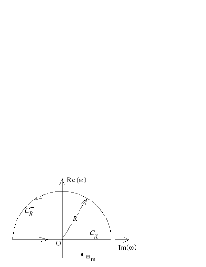
Figure 9: Contour $\mathcal{C}^{+}$.

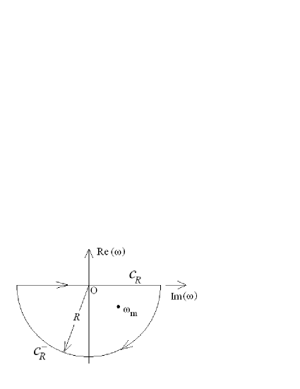
Figure 10: Contour $\mathcal{C}^{-}$.

Then

$$I_{\mathcal{C}^{+}}(\mathbf{x},t)=\int_{\mathcal{C}_{R}^{+}}\frac{1}{\omega-\omega_{m}^{o}}\exp(-i\omega t)d\omega+\int_{\mathcal{C}_{R}}\frac{1}{\omega-\omega_{m}^{o}}\exp(-i\omega t)d\omega~{},$$ (196)

$$I_{\mathcal{C}^{-}}(\mathbf{x},t)=\int_{\mathcal{C}_{R}^{-}}\frac{1}{\omega-\omega_{m}^{o}}\exp(-i\omega t)d\omega+\int_{\mathcal{C}_{R}}\frac{1}{\omega-\omega_{m}^{o}}\exp(-i\omega t)d\omega~{}.$$ (197)

However

$$I(\mathbf{x},t)=\lim_{R\rightarrow\infty}\int_{\mathcal{C}_{R}}\frac{1}{\omega-\omega_{m}^{o}}\exp(-i\omega t)d\omega~{},$$ (198)

so that, by virtue of Cauchy’s theorem

$$\lim_{R\rightarrow\infty}I_{\mathcal{C}^{+}}(\mathbf{x},t)=\lim_{R\rightarrow\infty}\int_{\mathcal{C}_{R}^{+}}\frac{1}{\omega-\omega_{m}^{o}}\exp(-i\omega t)d\omega+I(\mathbf{x},t)=0~{},$$ (199)

$$\lim_{R\rightarrow\infty}I_{\mathcal{C}^{-}}(\mathbf{x},t)=\lim_{R\rightarrow\infty}\int_{\mathcal{C}_{R}^{-}}\frac{1}{\omega-\omega_{m}^{o}}\exp(-i\omega t)d\omega+I(\mathbf{x},t)=-2\pi i~{}\text{Residue}\Big{|}_{\omega=\omega_{m}^{o}}~{},$$ (200)

However:

$$\Big{\|}\int_{\mathcal{C}_{R}^{+}}\frac{1}{\omega-\omega_{m}^{o}}\exp(-i\omega t)d\omega\Big{\|}<\int_{0}^{\pi}R\exp\left[Rt\sin\theta\right]d\theta\Big{\|}~{}~{};\\ ~{}~{}t<0~{}~{},~{}~{}R>>1~{},$$ (201)

so that (due to the fact that $\sin\theta\geq 0$ for $\theta\in[0,\pi]$)

$$\lim_{R\rightarrow\infty}\int_{\mathcal{C}_{R}^{+}}\frac{1}{\omega-\omega_{m}^{o}}\exp(-i\omega t)d\omega=0~{}~{};~{}~{}t<0~{},$$ (202)

whence (by virtue of (199)

$$I(\mathbf{x},t)=0~{}~{};~{}~{}t<0~{},$$ (203)

Similarly

$$\Big{\|}\int_{\mathcal{C}_{R}^{-}}\frac{1}{\omega-\omega_{m}^{o}}\exp(-i\omega t)d\omega\Big{\|}<\int_{2\pi}^{\pi}R\exp\left[Rt\sin\theta\right]d\theta\Big{\|}~{}~{};\\ ~{}~{}t>0~{}~{},~{}~{}R>>1~{},$$ (204)

so that (due to the fact that $\sin\theta\leq 0$ for $\theta\in[\pi,2\pi]$)

$$\lim_{R\rightarrow\infty}\int_{\mathcal{C}_{R}^{-}}\frac{1}{\omega-\omega_{m}^{o}}\exp\left(-i\omega t\right)d\omega=0~{}~{};~{}~{}t>0~{},$$ (205)

whence (by virtue of (200)

$$I(\mathbf{x},t)=-2\pi i~{}\text{Residue}\Big{|}_{\omega=\omega_{m}^{o}}=-2\pi i\exp(-i\omega t)~{}~{};~{}~{}t>0~{}.$$ (206)

Thus,

$$I(\mathbf{x},t)=-2\pi i\exp(-i\omega_{m}^{o}t)H(t)~{}$$ (207)

wherein $H$ is the Heaviside function ($H(\chi)=0~{};~{}\chi<0$ and $H(\chi)=1~{};~{}\chi>0$).

It follows from (164) that

$$F_{1}(t_{1})=2\pi\sum_{m\in\mathbb{Z}}\frac{\exp(-i\omega_{m}^{o}t_{1})}{\dot{D}(\omega_{m}^{o},s^{i})}H(t_{1})~{}.$$ (208)

Due to the fact that $H(-t_{1})=0~{};~{}t_{1}>0$,

$$F_{1}(-t_{1})=0~{}~{};~{}~{}t_{1}>0~{},$$ (209)

whence

$$u_{3}^{1\pm}(\mathbf{x},t)=\frac{1}{2\pi}\int_{0}^{\infty}F_{1}(t_{1})F_{2}\left(\tau^{1\pm}(\mathbf{x},t,s^{i})-t_{1}\right)dt_{1}~{},$$ (210)

or, more explicitly

$$u_{3}^{1\pm}(\mathbf{x},t)=\mathcal{A}\sum_{m\in\mathbb{Z}}\frac{1}{\dot{D}(\omega_{m}^{o},s^{i})}\int_{0}^{\infty}\left[-1+2\alpha^{2}(\tau^{1\pm}(\mathbf{x},t,s^{i})-t_{1}-\beta)^{2}\right]\times\\ \exp[-i\omega_{m}^{o}t_{1}-\alpha^{2}(\tau^{1\pm}(\mathbf{x},t,s^{i})-t_{1}-\beta)^{2}]dt_{1}~{}.$$ (211)

At this point, we recall that (with obvious shorthand notation):

$$\omega_{m}^{o}=\omega_{m}^{o^{\prime}}+i\omega_{m}^{o"}~{}~{},~{}~{}\omega_{m}^{o^{\prime}}=(2m+1)\frac{\pi}{2\gamma}~{}~{},~{}~{}\omega_{m}^{o"}=\frac{1}{2\gamma}\ln\left(\frac{a-b}{a+b}\right)=\omega^{o"}<0~{},$$ (212)

$$\dot{D}(\omega_{m}^{o},s^{i})=i(-1)^{m}\gamma\frac{b^{2}-a^{2}}{a}\cosh(\gamma\omega_{m}^{o"})=i(-1)^{m}\mathrm{\dot{D}}(s^{i})~{}~{},~{}~{}\mathrm{\dot{D}}(s^{i})=\gamma\frac{b^{2}-a^{2}}{a}\cosh(\gamma\omega^{o"})~{}.$$ (213)

Remark
We notice that $\omega_{m}^{o"}=\omega^{o"}$ and $\mathrm{\dot{D}}(s^{i})$ are independent of $m$.

Thus, we can write (211) as

$$u_{3}^{1\pm}(\mathbf{x},t)=\frac{\mathcal{A}}{i\mathrm{\dot{D}}}\int_{0}^{\infty}S(t_{1})\left[-1+2\alpha^{2}(\tau^{1\pm}(\mathbf{x},t,s^{i})-t_{1}-\beta)^{2}\right]\times\\ \exp[-i\omega_{m}^{o}t_{1}-\alpha^{2}(\tau^{1\pm}(\mathbf{x},t,s^{i})-t_{1}-\beta)^{2}]dt_{1}~{},$$ (214)

wherein

$$S(t_{1})=\sum_{m=-\infty}^{\infty}(-1)^{m}\exp(-i\omega_{m}^{o}t_{1})=\exp(\omega^{o"}t_{1})\sum_{m=-\infty}^{\infty}(-1)^{m}\exp\left[-i(2m+1)\frac{\pi}{2\gamma}t_{1}\right]~{}.$$ (215)

Thus:

$$u_{3}^{1\pm}(\mathbf{x},t)=\frac{\mathcal{A}}{i\mathrm{\dot{D}}}\int_{0}^{\infty}\sigma(t_{1})\left[-1+2\alpha^{2}(\tau^{1\pm}(\mathbf{x},t,s^{i})-t_{1}-\beta)^{2}\right]\times\\ \exp[\omega^{o"}t_{1}-\alpha^{2}(\tau^{1\pm}(\mathbf{x},t,s^{i})-t_{1}-\beta)^{2}]dt_{1}~{},$$ (216)

wherein

$$\sigma(t_{1})=\sum_{m=-\infty}^{\infty}(-1)^{m}\exp\left[-i(2m+1)\frac{\pi}{2\gamma}t_{1}\right]=\exp\left(-i\frac{\pi}{2\gamma}t_{1}\right)\sum_{m=-\infty}^{\infty}\exp\left[i\frac{m\pi}{\gamma}(\gamma-t_{1})\right]~{}.$$ (217)

We make use of the Poisson sum formula (Morse and Feshbach, 1953)

$$\sum_{m=-\infty}^{\infty}\exp\left(imdx\right)=\frac{2\pi}{d}\sum_{m=-\infty}^{\infty}\delta\left(x+\frac{2m\pi}{d}\right)~{},$$ (218)

wherein we take $d=\frac{\pi}{\gamma}$ and $x=\gamma-t_{1}$, to obtain

$$\sum_{m=-\infty}^{\infty}\exp\left[i\frac{m\pi}{\gamma}(\gamma-t_{1})\right]=2\gamma\sum_{m=-\infty}^{\infty}\delta\left(\gamma-t_{1}+2m\gamma\right)=2\gamma\sum_{m=-\infty}^{\infty}\delta\left(t_{1}-(2m+1)\gamma\right)~{}.$$ (219)

But (recall that $\gamma>0$) $t_{1}=(2m+1)\gamma<0$ for $m<0$, so that

$$\sum_{m=-\infty}^{\infty}\exp\left[i\frac{m\pi}{\gamma}(\gamma-t_{1})\right]=2\gamma\sum_{m=0}^{\infty}\delta\left(\gamma-t_{1}+2m\gamma\right)~{}~{};~{}~{}t_{1}\geq 0~{},$$ (220)

whence

$$\sigma(t_{1})=2\gamma\exp\left(-i\frac{\pi}{2\gamma}t_{1}\right)\sum_{m=0}^{\infty}\delta\left(t_{1}-(2m+1)\gamma\right)~{}~{};~{}~{}t_{1}\geq 0~{},$$ (221)

or, on account of the properties of the Dirac delta distribution,

$$\sigma(t_{1})=2\gamma\sum_{m=0}^{\infty}\exp\left(-i\frac{\pi}{2\gamma}(2m+1)\gamma\right)\delta\left(t_{1}-(2m+1)\gamma\right)=\\ -2i\gamma\sum_{m=0}^{\infty}(-1)^{m}\delta\left(t_{1}-(2m+1)\gamma\right)=~{}~{};~{}~{}t_{1}\geq 0~{}.$$ (222)

Consequently:

$$u_{3}^{1\pm}(\mathbf{x},t)=\frac{-2i\gamma\mathcal{A}}{i\mathrm{\dot{D}}}\sum_{m=0}^{\infty}(-1)^{m}\int_{0}^{\infty}\delta\left(t_{1}-(2m+1)\gamma\right)\left[-1+2\alpha^{2}(\tau^{1\pm}(\mathbf{x},t,s^{i})-t_{1}-\beta)^{2}\right]\times\\ \exp[\omega^{o"}t_{1}-\alpha^{2}(\tau^{1\pm}(\mathbf{x},t,s^{i})-t_{1}-\beta)^{2}]dt_{1}~{},$$ (223)

or finally, on account of the sifting property of the Dirac delta distribution,

$$u_{3}^{1\pm}(\mathbf{x},t)=\frac{-2\gamma\mathcal{A}}{\mathrm{\dot{D}}}\sum_{m=0}^{\infty}(-1)^{m}\left[-1+2\alpha^{2}\{\tau^{1\pm}(\mathbf{x},t,s^{i})-(2m+1)\gamma-\beta\}^{2}\right]\times\\ \exp[\omega^{o"}(2m+1)\gamma-\alpha^{2}\{\tau^{1\pm}(\mathbf{x},t,s^{i})-(2m+1)\gamma-\beta\}^{2}]~{}.$$ (224)

The terms of the series decrease exponentially with $m$ so that the series can be approximated by a sum of $M+1$ terms

$$u_{3}^{1\pm}(\mathbf{x},t)\approx\frac{-2\gamma\mathcal{A}}{\mathrm{\dot{D}}}\sum_{m=0}^{M}(-1)^{m}\left[-1+2\alpha^{2}\{\tau^{1\pm}(\mathbf{x},t,s^{i})-(2m+1)\gamma-\beta\}^{2}\right]\times\\ \exp[\omega^{o"}(2m+1)\gamma-\alpha^{2}\{\tau^{1\pm}(\mathbf{x},t,s^{i})-(2m+1)\gamma-\beta\}^{2}]~{},$$ (225)

which is the form adopted in the numerical applications of this method.

Remark
As shown in the following section, the pole-residue convolution method gives rise to the correct solution in all cases.

4.3.5 Comparison of the three methods for evaluating the Fourier transform intervening in the temporal response for Ricker pulse excitation

Figure 11: Time history at $\mathbf{x}=(0,0)$ computed by the rectangular quadrature method for an ”anomalous” pulse. $\mathcal{A}=1$, $\alpha=1$, $\beta=1$, $\gamma=1$, $a=1$, $b=0.7$, $\omega_{max}=30Hz$, $L=301$.

Figure 12: Time history at $\mathbf{x}=(0,0)$ computed by the power series method for an ”anomalous” pulse. $\mathcal{A}=1$, $\alpha=1$, $\beta=1$, $\gamma=1$, $a=1$, $b=0.7$, $M=10$.

Figure 13: Time history at $\mathbf{x}=(0,0)$ computed by the pole-residue convolution method for an ”anomalous” pulse. $\mathcal{A}=1$, $\alpha=1$, $\beta=1$, $\gamma=1$, $a=1$, $b=0.7$, $M=2$.

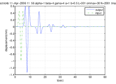
Figure 14: Time history at $\mathbf{x}=(0,0)$ computed by the rectangular quadrature method for separated pulses. $\mathcal{A}=1$, $\alpha=1$, $\beta=4$, $\gamma=4$, $a=1$, $b=0.5$, $\omega_{max}=30Hz$, $L=301$.

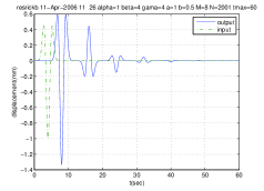
Figure 15: Time history at $\mathbf{x}=(0,0)$ computed by the power series method for separated pulses. $\mathcal{A}=1$, $\alpha=1$, $\beta=4$, $\gamma=4$, $a=1$, $b=0.5$, $M=8$.

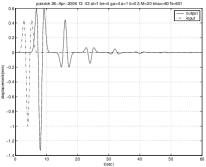
Figure 16: Time history at $\mathbf{x}=(0,0)$ computed by the pole-residue convolution method for separated pulses. $\mathcal{A}=1$, $\alpha=1$, $\beta=4$, $\gamma=4$, $a=1$, $b=0.5$, $M=20$.

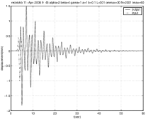
Figure 17: Time history at $\mathbf{x}=(0,0)$ computed by the rectangular quadrature method for merged pulses. $\mathcal{A}=1$, $\alpha=2$, $\beta=4$, $\gamma=1$, $a=1$, $b=0.1$, $\omega_{max}=30Hz$, $L=301$.

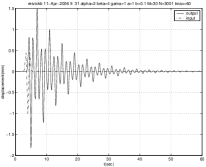
Figure 18: Time history at $\mathbf{x}=(0,0)$ computed by the power series method for merged pulses. $\mathcal{A}=1$, $\alpha=2$, $\beta=4$, $\gamma=1$, $a=1$, $b=0.1$, $M=30$.

Figure 19: Time history at $\mathbf{x}=(0,0)$ computed by the pole-residue convolution method for merged pulses. $\mathcal{A}=1$, $\alpha=2$, $\beta=4$, $\gamma=1$, $a=1$, $b=0.1$, $M=50$.

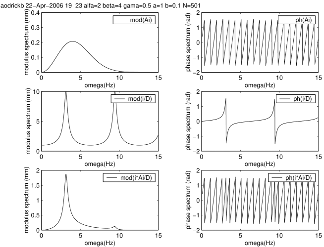
Figure 20: Spectrum of displacement response at $\mathbf{x}=(0,0)$. $\mathcal{A}=1$, $\alpha=2$, $\beta=4$, $\gamma=0.5$, $a=1$, $b=0.1$, corresponding to the case of a quasi-monochromatic pulse. The left-hand curves pertain to moduli, and the right hand curves to phases of the spectra.

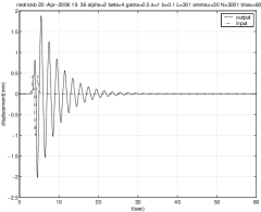
Figure 21: Time history at $\mathbf{x}=(0,0)$ computed by the rectangular quadrature method for a quasi monochromatic pulse. $\mathcal{A}=1$, $\alpha=2$, $\beta=4$, $\gamma=0.5$, $a=1$, $b=0.1$, $\omega_{max}=30Hz$, $L=301$.

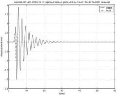
Figure 22: Time history at $\mathbf{x}=(0,0)$ computed by the power series method for a quasi monochromatic pulse. $\mathcal{A}=1$, $\alpha=2$, $\beta=4$, $\gamma=0.5$, $a=1$, $b=0.1$, $M=30$.

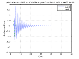
Figure 23: Time history at $\mathbf{x}=(0,0)$ computed by the pole-residue convolution method for a quasi monochromatic pulse. $\mathcal{A}=1$, $\alpha=2$, $\beta=4$, $\gamma=0.5$, $a=1$, $b=0.1$, $M=50$.

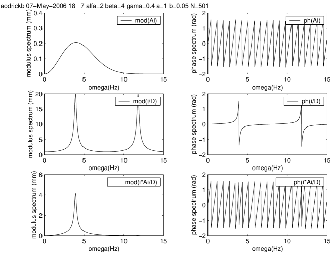
Figure 24: Spectrum of displacement response at $\mathbf{x}=(0,0)$. $\mathcal{A}=1$, $\alpha=2$, $\beta=4$, $\gamma=0.4$, $a=1$, $b=0.05$, corresponding to the case of a monochromatic pulse. The left-hand curves pertain to moduli, and the right hand curves to phases of the spectra.

Figure 25: Time history at $\mathbf{x}=(0,0)$ computed by the rectangular quadrature method for a monochromatic pulse. $\mathcal{A}=1$, $\alpha=2$, $\beta=4$, $\gamma=0.4$, $a=1$, $b=0.05$, $\omega_{max}=30Hz$, $L=301$.

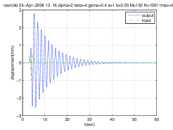
Figure 26: Time history at $\mathbf{x}=(0,0)$ computed by the power series method for a monochromatic pulse. $\mathcal{A}=1$, $\alpha=2$, $\beta=4$, $\gamma=0.4$, $a=1$, $b=0.05$, $M=150$.

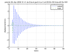
Figure 27: Time history at $\mathbf{x}=(0,0)$ computed by the pole-residue convolution method for a monochromatic pulse. $\mathcal{A}=1$, $\alpha=2$, $\beta=4$, $\gamma=0.4$, $a=1$, $b=0.05$, $M=100$.

The three methods are: i) the rectangle quadrature method, ii) the power series method, and iii) the complex frequency pole-residue convolution method.

In the set of figures 11, 12, 13 (for a so-called ”anomalous” pulse), 14, 15, 16 (for separated pulses), and 17, 18, 19 (for merged pulses) we exhibit the time history of displacement response at the location $\mathbf{x}=(0,0)$ on the ground plane.

We next choose what seems a typical geophysically-interesting situation (at least in the frequency domain) depicted in fig. 20. The corresponding time-domain responses are given in figures 21, 22, 23.

As a last example, we choose a more idealized (and less realizable due to the very large contrast of physical properties it implies between the layer and the substratum) geophysical example, the frequency response of which is depicted in fig. 24. The corresponding time-domain responses are given in figures 25, 26, 27.

Remark
We notice that all the three methods again give the same results.

Remark
Note that the relatively-long duration and monochromatic nature of the temporal response in figs. 25, 26, 27 are due to the large Q single-spike nature of the frequency response, the latter being a result of the large contrast of physical properties and the fact that only one $1/D$ spike is located within the significant part of the spectrum of the Ricker pulse.

4.3.6 Discussion

Remark
The rectangle quadrature method, embodied in (119), produces a purely-numerical result which gives no insight as to the physical nature of this response. It was proposed only as a reference solution by which the other two methods could be judged, at least on a numerical basis. This rectangle quadrature method is certainly not optimal, even from the purely-numerical point of view, but obviously one of the simplest to explain and program.

Remark
By inspection of (145) and comparison with (95), we see that the power series method gives rise to an expression of the time history response to a Ricker pulse that is a sum of displaced (and increasingly-attenuated) Ricker pulses. This is what one would expect on an intuitive basis for a dispersionless configuration. Thus, it would seem that the power series method is the most appropriate one, at least in the situation in which the successive pulses are well-separated. However, in the case in which the successive pulses are not well-separated, intuition is lost (especially when a long-duration quasi-monochromatic response is produced) and the power series picture reflects this fact, although it still gives rise to the correct numerical response. However, the power series method cannot be applied when $D\approx 0$ as is the case in which Love modes are excited. This is the reason why the pole-residue convolution method was proposed.

Remark
The pole-residue convolution solution in (225) expresses the time history of response as a weighted sum of displaced Ricker pulses (the latter would probably be distorted Ricker pulses in the presence of dispersion). This is close to being intuitive, but what is less intuitive is the fact that the displacements are a function of the real part of the complex zeros of the equation $D(\omega,s^{i})=0$ and the weight functions are expressed in terms of the imaginary part of the complex zeros of the equation $D(\omega,s^{i})=0$.

The fact that the essential features (peak values and duration, amongst others) of the time history are directly-related to the complex eigenvalues of the structure is the essential result we were aiming at in this contribution.

The most important parameter is the imaginary part of the eigenvalues since it regulates the height of the succesive Ricker pulses and therefore determines the duration of the time domain response. This parameter is a measure of radiation damping (which is leakage of energy into the substratum, an attenuation mechanism that exists even in the absence of material dissipation in the layer).

The pole-residue convolution expression of the time history appears to be similar to the one obtained by the power series method, but the latter method is not applicable when $D(\omega,s^{i})=0$ for real eigenvalues in the absence of dissipation (i.e., the situation in which it is possible to excite Love modes (Groby and Wirgin 2005a,b)); moreover, the power series method does not enable one to predict the duration in an obvious way.

Remark
Some of the numerical results included in this work are rather unexpected. For instance, the time histories given in figs. 17, 18, 19 have quite long durations that one would not expect to occur for a case in which modes cannot be excited. Actually, this long duration is due to the fact that the only attenuative action in this work is the one due to radiation damping. The duration would be shorter if material dissipation (i.e., viscoelasticity) were taken into account in the layer and/or the contrast between $a$ and $b$ were smaller.

5 Conclusions

The main result of this contribution is that the three methods give rise to the same solutions for a large variety of scattering configurations.

The complex frequency pole-residue convolution method turns out to be the most interesting method since: i) it is numerically-efficient, ii) it is explicit as concerns the understanding and quantification of the duration of the time domain response, iii) it can be employed even in the case in which genuine resonances (due to mode excitation) are produced.

The part of this study concerning the complex frequency pole residue convolution method constitutes a correction of its counterpart in our previous publications (Groby and Wirgin, 2005a) and (Groby and Wirgin 2005b). A somewhat similar approach, although applied to a fluid layer in a fluid host, is that of (Conoir, 1987).

Work remains to be done to take into account dispersion and damping of the material in the layer.

The natural follow-up of this study is to elucidate theoretically the nature of the time histories of response not only for the case (the one treated herein) in which the configuration is unable to excite (e.g., Love) modes, but also in the case in which such modes can be excited (Groby and Wirgin 2005a,b).

References

• Conoir J.-M., Réflexion et transmission par une plaque fluide, in La Diffusion Acoustique, Gespa N. (ed.), Cedocar Paris Armées, Paris, 1987, 105-132.

• Groby J.-P. and Wirgin A., 2D ground motion at a soft viscoelastic layer/hard substratum site in response to SH cylindrical seismic waves radiated by near and distant line sources. I. Theory, Geophys.J.Int., 2005, 163, 165-191.

• Groby J.-P. and Wirgin A., 2D ground motion at a soft viscoelastic layer/hard substratum site in response to SH cylindrical seismic waves radiated by near and distant line sources. II. Computations, Geophys.J.Int., 2005, 163, 192-224.

• Hodgman C.D.(ed.), CRC Standard Mathematical Tables, Chemical Rubber Publ. Co., Cleveland, 1957, 304.

• Morse P.M. and Feshbach H., Methods of Theoretical Physics, Mc Graw-Hill, New York, 1953.

• Sanchez-Sesma F.J, Diffraction of elastic SH waves by wedges, Bull.Seism.Soc.Am., 1985, 75, 1435-1446.