Thin film dynamics on a vertically rotating disk partially immersed in a liquid bath

K. Afanasiev$\,{}^{1}$, A. Münch$\,{}^{2}$, B. Wagner$\,{}^{1}$

¹ Weierstrass Institute for Applied Analysis and Stochastics,
   Mohrenstrasse 39, 10117 Berlin, Germany
² Institute of Mathematics, Humboldt University, 10099 Berlin, Germany

Abstract

The axisymmetric flow of a thin liquid film is considered for the problem of a vertically rotating disk that is partially immersed in a liquid bath. A model for the fully three-dimensional free-boundary problem of the rotating disk, that drags a thin film out of the bath is set up. From this, a dimension-reduced extended lubrication approximation that includes the meniscus region is derived. This problem constitutes a generalization of the classic drag-out and drag-in problem to the case of axisymmetric flow. The resulting nonlinear fourth-order partial differential equation for the film profile is solved numerically using a finite element scheme. For a range of parameters steady states are found and compared to asymptotic solutions. Patterns of the film profile, as a function of immersion depth and angular velocity are discussed.

1 Introduction

The problem of rotating thin film flows has been investigated extensively, both theoretically and experimentally, due to the many technological applications. Starting with the work by Emslie et al. [4], various aspects of this type of surface tension driven flow, influencing the shape and stability of the film, have been studied. These include for example non-Newtonian effects the paper by [5], for evaporation [15] and Coriolis force [11], [12], see also [13] for a recent experimental study. As with those studies most of them dealt with a configuration where the fluid layer is moving on a horizontally rotating disk. Making use of the large scale separation between the small thickness of the film and the length scale of the evolving patterns, thin film models where used to derive dimension-reduced models of the underlying three-dimensional free boundary problems.

For the situation of a disk that is partially immersed in a bath of liquid and rotating about the horizontal axis, thereby dragging out a thin film onto the disk (see figure 1), there are far fewer studies even though this configuration is typical for many applications. For example, for oil disk skimmers, which is used as an effective device for oil recovery and as an alternative to toxic chemical dispersants, used after an offshore oil spill. Another application is the fluid dynamical aspects in connection with the synthesis of Polyethylenterephthalat(PET) in polycondensation reactors. These typically consist of a horizontal cylinder that is partially filled with polymer melt and contains disks rotating about the horizontal axis of the cylinder, thus picking up and spreading the melt in form of a thin film over a large area of the disks.

These type of problems always involve a meniscus region, that connects the thin film to the liquid bath and a spacially oscillating region shortly before the film is dragged into the bath again. In these two regions the scale separation is not large anymore and hence the lubrication approximation is not valid there. Nevertheless, the meniscus does play the crucial role of fixing the height of the dragged out film and therefore both, the meniscus region and similarly the drag-in region that connecting the thin film to the liquid bath must be accounted for in a dimension-reduced model, which we will derive in this paper. The classic and far simpler setting of the free boundary problems for falling and rising thin film flows on vertical as well as inclined planes has been investigated as early as in the work by Landau and Levich [9]. Their work lead to the prediction of the height and shape of the thin film emerging out of the meniscus. The results were improved by Wilson [18] and for the case of a Marangoni-driven rising film by [17] and Münch [10], using systematic asymptotic analysis in the limit of small capillary numbers. Such asymptotic analyses can be applied to more complex situations such as the problem we consider here for the vertically rotating disk.

Previous studies for this problem was performed by Christodoulo et al. [1]. The employed the analysis of the meniscus region by Wilson [18] for the problem of flow control for rotating oil disk skimmers. Their study did not extend further into the thin film region on the remainder of the disk. However, for many applications it is important to answer questions for example on the maximum surface area of the film profile or the optimum volume of liquid that is dragged out and spread on the disk, for which the predictions resulting from the simple drag-out study will not be sufficient. Up to now no complete model for the vertically rotating disk, including its numerical solution has appeared. This will be the topic of this paper.

In section 2 we set up the corresponding three-dimensional free boundary problem. A fully three-dimensional analysis of such flows represents a very time consuming task, analytically and numerically. To be able to perform systematic parameter studies we therefore exploit the large separation of scales to obtain a dimension-reduced lubrication model. This model will then be extended to match to the flow field in the meniscus region. For the resulting model we develop in section 3 a weak formulation and a corresponding finite element discretization for the full dynamical problem. Since we want to address here issues of maximum surface area of the film profile or the optimum volume of liquid that is dragged out, we are intersted mainly in the long-time behavior. This will be the focus of the following sections. In section 4 we solve and discuss for a range of parameters the emerging steady state solutions. Their shapes near the meniscus region are then compared to the asymptotic solution of the corresponding drag-out problem. Away from the liquid bath the film profile is compared to asymptotic solutions, by using the methods of characteristics. For both regions excellent agreement is found. Finally, we discuss the novel patterns for the film profile as the immersion depth, or the angular velocity is varied.

2 Formulation

2.1 Governing Equations

We consider the isothermal flow of an incompressible, viscous liquid on a vertical disk rotating in the vertical plane and partially immersed in the liquid. We assume that the disk of radius $R$ rotates with the angular velocity $\Omega$ about a horizontal axis, which has distance $a$ to the bath, see figure 1.

Figure 1: Configuration of a single disk within a PET-reactor

To formulate the problem, we introduce cylindrical polar coordinates $(r,\theta,z)$ in the laboratory frame of reference. We let the liquid velocity vector have components $(u,v,w)$ and let $\mathbf{\omega}$ denote the angular velocity vector with components $(0,0,\Omega)$. The momentum balance equations can be expressed as

$$\rho\left[u_{t}+uu_{r}+\frac{v}{r}u_{\theta}-\frac{v^{2}}{r}+wu_{z}\right] = -p_{r}+\mu\left[\bigtriangleup u-\frac{2v_{\theta}}{r^{2}}-\frac{u}{r^{2}}\right]-\rho g\sin\theta\qquad$$

$$\rho\left[v_{t}+uv_{r}+\frac{v}{r}v_{\theta}+\frac{uv}{r}+wv_{z}\right] = -\frac{p_{\theta}}{r}+\mu\left[\bigtriangleup v+\frac{2u_{\theta}}{r^{2}}-\frac{v}{r^{2}}\right]-\rho g\cos\theta\qquad$$

$$\rho\left[w_{t}+uw_{r}+\frac{v}{r}w_{\theta}+ww_{z}\right] = -p_{z}+\mu\bigtriangleup w\qquad$$ (2.1c)

where

$$\bigtriangleup f=\frac{1}{r}\left(rf_{r}\right)_{r}+\frac{f_{\theta\theta}}{r^{2}}+f_{zz}.$$ (2.2)

We let $\rho$, $\mu$ and $p$ denote the density, dynamic shear viscosity and the pressure of the liquid, respectively. The external force here is gravity and $g$ denotes the gravitational constant.

The continuity equation is

$$\frac{1}{r}(ru)_{r}+\frac{1}{r}v_{\theta}+w_{z}=0.$$ (2.3)

For the boundary condition at the surface of the disk, i.e. $z=0$, that rotates with the velocity $\Omega$, we impose the no-slip condition for $u$ and $v$ and the impermeability condition for $w$. Hence, we have

$$u=0,\qquad v=r\Omega,\qquad w=0,$$ (2.4)

respectively.

At the free boundary $z=h(r,\theta,t)$ we require the normal stress condition

$${\bf n}\,\Pi\,{\bf n}=2\sigma\kappa,$$ (2.5)

the tangential stress conditions

$${\bf n}\,\Pi\,{\bf t}_{i}=0,\quad\quad\mbox{where}\quad i=1,2,$$ (2.6)

and the kinematic condition

$$h_{t}=w-u_{|h}h_{r}-\frac{1}{r}v_{|h}h_{\theta},$$ (2.7)

which can also be written, upon using the continuity equation, as

$$h_{t}=-\frac{1}{r}\frac{\partial}{\partial r}\,r\int^{h}_{0}u\,dz-\frac{1}{r}\frac{\partial}{\partial\theta}\int^{h}_{0}v\,dz.$$ (2.8)

The normal and the tangential vectors in radial and angular direction are given by

$${\bf n}=\frac{\left(-h_{r},-h_{\theta}/r,1\right)}{\left(1+h_{r}^{2}+h_{\theta}^{2}/r^{2}\right)^{1/2}},\quad{\bf t}_{1}=\frac{\left(1,0,h_{r}\right)}{\left(1+h_{\theta}^{2}/r^{2}\right)^{1/2}},\quad{\bf t}_{2}=\frac{\left(0,1,h_{\theta}/r\right)}{\left(1+h_{\theta}^{2}/r^{2}\right)^{1/2}},$$ (2.9)

respectively. The stress tensor $\Pi$ is symmetric and has the components

$$\begin{array}[]{lll}\Pi_{rr}=-p+2\mu\,u_{r},&\Pi_{\theta\theta}=-p+2\mu\left(\displaystyle\frac{v_{\theta}}{r}+\frac{u}{r}\right),&\Pi_{zz}=-p+2\mu w_{z},\\ \\ \Pi_{r\theta}=\mu\left(\displaystyle\frac{u_{\theta}}{r}+v_{r}-\displaystyle\frac{v}{r}\right),&\Pi_{\theta z}=\mu\left(v_{z}+\displaystyle\frac{w_{\theta}}{r}\right),&\Pi_{rz}=\mu\left(w_{r}+u_{z}\right).\end{array}$$ (2.13)

Finally, we assume surface tension to be constant and denote it by $\sigma$ and the mean curvature is given by

$$\kappa=\frac{1}{2}\left(\frac{1}{r}\frac{\partial}{\partial r}\frac{rh_{r}}{\left(1+h_{r}^{2}+h_{\theta}^{2}/r^{2}\right)^{1/2}}+\frac{1}{r}\frac{\partial}{\partial\theta}\frac{h_{\theta}/r}{\left(1+h_{r}^{2}+h_{\theta}^{2}/r^{2}\right)^{1/2}}\right).$$ (2.14)

Using this in equations (2.5) and (2.6) we obtain the boundary conditions for the normal stress

$$-p+\frac{2\mu}{1+h^{2}_{r}+h_{\theta}^{2}/r^{2}}\left[\left(\frac{u_{\theta}}{r}+v_{r}-\frac{v}{r}\right)\frac{h_{r}h_{\theta}}{r}\right.$$

$$\left.-(w_{r}+u_{z})h_{r}-\left(v_{z}+\frac{w_{\theta}}{r}\right)\frac{h_{\theta}}{r}+u_{r}h_{r}^{2}+(v_{\theta}+u)\frac{h_{\theta}^{2}}{r^{3}}+w_{z}\right]$$ (2.15)

$$=\sigma\left[\frac{1}{r}\frac{\partial}{\partial r}\frac{rh_{r}}{\left(1+h_{r}^{2}+h_{\theta}^{2}/r^{2}\right)^{1/2}}+\frac{1}{r}\frac{\partial}{\partial\theta}\frac{h_{\theta}/r}{\left(1+h_{r}^{2}+h_{\theta}^{2}/r^{2}\right)^{1/2}}\right],$$

the tangential stress condition in radial direction

$$2(w_{z}-u_{r})h_{r}-\left(\frac{u_{\theta}}{r}+v_{r}-\frac{v}{r}\right)\frac{h_{\theta}}{r}$$

$$+(w_{r}+u_{z})(1-h^{2}_{r})-\left(v_{z}+\frac{w_{\theta}}{r}\right)\frac{h_{r}h_{\theta}}{r}=0$$

and the tangential stress condition in angular direction

$$2\left(w_{z}-\frac{v_{\theta}}{r}-\frac{u}{r}\right)\frac{h_{\theta}}{r}-\left(\frac{u_{\theta}}{r}+v_{r}-\frac{v}{r}\right)h_{r}$$

$$+\left(v_{z}+\frac{w_{\theta}}{r}\right)\left(1-\frac{h^{2}_{\theta}}{r^{2}}\right)-\left(w_{r}+u_{z}\right)\frac{h_{r}h_{\theta}}{r}=0$$

2.2 Lubrication approximation

The solution of the above three-dimensional free boundary problem represents, analytically and numerically a time consuming task for making accurate parameter studies. The key idea that we make use of here in order to obtain a mathematically and numerically tractable problem, is the exploitation of the scale separation in most parts of this flow problem.

We begin by introducing dimensionsless variables and set

$$\begin{array}[]{lll}r=L\bar{r},&\theta=\bar{\theta},&z=H\bar{z},\\ u=U\bar{u},&v=U\bar{v},&w=W\bar{w},\\ p=P\bar{p},&t=T\bar{t}.&\end{array}$$ (2.18)

The characteristic velocity $U$ is set by the velocity of the rotating disk. For given radius $R$ of the disk we let

$$U=R\Omega.$$ (2.19)

We determine the scale for the characteristic height $H$ by balancing the dominant viscous term with gravitational term in the $u$-momentum equation, which yields

$$H=\sqrt{\frac{\mu U}{\rho g}}.$$ (2.20)

Furthermore, we require that the pressure must also balance the dominant viscous term, so that

$$P=\frac{\mu UL}{H^{2}}$$ (2.21)

and that surface tension is important, so that from the normal stress boundary condition we find

$$P=\frac{\sigma H}{L^{2}}.$$ (2.22)

This yields the scale for $L$ as

$$L=\frac{H}{\displaystyle\left(\frac{\mu U}{\sigma}\right)^{1/3}}$$ (2.23)

and the time scale is fixed by $T=L/U$.

We assume that the liquid film is very thin and that the velocity in the direction normal to the disk is much smaller than along the disk. We let

$$\varepsilon=\frac{H}{L}\ll 1$$ (2.24)

be a small parameter and $W=\varepsilon U$. Note that this also means that the capillary number Ca is small,

$$\mbox{Ca}^{1/3}=\left(\frac{\mu U}{\sigma}\right)^{1/3}=\frac{H}{L}\ll 1.$$ (2.25)

With these scales the non-dimensional equations are

$$\varepsilon^{2}\mbox{Re}\left[u_{t}+uu_{r}+\frac{v}{r}u_{\theta}-\frac{v^{2}}{r}+wu_{z}\right] = -p_{r}+u_{zz}-\sin\theta\qquad$$

$$+\varepsilon^{2}\left[\frac{(ru_{r})_{r}}{r}+\frac{u_{\theta\theta}}{r^{2}}-\frac{2v_{\theta}}{r^{2}}-\frac{u}{r^{2}}\right]$$

$$\varepsilon^{2}\mbox{Re}\left[v_{t}+uv_{r}+\frac{v}{r}v_{\theta}+\frac{uv}{r}+wv_{z}\right] = -\frac{p_{\theta}}{r}+v_{zz}-\cos\theta\qquad$$

$$+\varepsilon^{2}\left[\frac{(rv_{r})_{r}}{r}+\frac{v_{\theta\theta}}{r^{2}}+\frac{2u_{\theta}}{r^{2}}-\frac{v}{r^{2}}\right]$$

$$\varepsilon^{4}\mbox{Re}\left[w_{t}+uw_{r}+\frac{v}{r}w_{\theta}+ww_{z}\right] = -p_{z}+\varepsilon^{2}w_{zz}+\varepsilon^{4}\left[\frac{(rw_{r})_{r}}{r}+\frac{w_{\theta\theta}}{r^{2}}\right]\qquad$$

where the Reynolds number is Re$=\rho\,UL/\mu$ and we have dropped the ’$\,\,\bar{\,}$ ’s.

The boundary conditions at the disk, $z=0$ are

$$u=0,\qquad v=\alpha r,\qquad w=0,$$ (2.27)

where $\alpha=L/R$.

The boundary conditions at the free liquid surface $z=h(r,\theta,t)$ are the conditions for normal and tangential stresses

$$-p+\frac{2\varepsilon^{2}}{1+\varepsilon^{2}h^{2}_{r}+\varepsilon^{2}h_{\theta}^{2}/r^{2}}\left[\varepsilon^{2}\left(\frac{u_{\theta}}{r}+v_{r}-\frac{v}{r}\right)\frac{h_{r}h_{\theta}}{r}\right.$$ (2.28)

$$\left.-(\varepsilon^{2}w_{r}+u_{z})h_{r}-\left(v_{z}+\varepsilon^{2}\frac{w_{\theta}}{r}\right)\frac{h_{\theta}}{r}+\varepsilon^{2}u_{r}h_{r}^{2}+\varepsilon^{2}(v_{\theta}+u)\frac{h_{\theta}^{2}}{r^{3}}+w_{z}\right]$$

$$=\left[\frac{1}{r}\frac{\partial}{\partial r}\frac{rh_{r}}{\left(1+\varepsilon^{2}h_{r}^{2}+\varepsilon^{2}h_{\theta}^{2}/r^{2}\right)^{1/2}}+\frac{1}{r}\frac{\partial}{\partial\theta}\frac{h_{\theta}/r}{\left(1+\varepsilon^{2}h_{r}^{2}+\varepsilon^{2}h_{\theta}^{2}/r^{2}\right)^{1/2}}\right],$$

$$2\varepsilon^{2}(w_{z}-u_{r})h_{r}-\varepsilon^{2}\left(\frac{u_{\theta}}{r}+v_{r}-\frac{v}{r}\right)\frac{h_{\theta}}{r}$$

$$+(\varepsilon^{2}w_{r}+u_{z})(1-\varepsilon^{2}h^{2}_{r})-\varepsilon^{2}\left(v_{z}+\varepsilon^{2}\frac{w_{\theta}}{r}\right)\frac{h_{r}h_{\theta}}{r}=0$$

$$2\varepsilon^{2}\left(w_{z}-\frac{v_{\theta}}{r}-\frac{u}{r}\right)\frac{h_{\theta}}{r}-\varepsilon^{2}\left(\frac{u_{\theta}}{r}+v_{r}-\frac{v}{r}\right)h_{r}$$

$$+\left(v_{z}+\varepsilon^{2}\frac{w_{\theta}}{r}\right)\left(1-\varepsilon^{2}\frac{h^{2}_{\theta}}{r^{2}}\right)-\varepsilon^{2}\left(\varepsilon^{2}w_{r}+u_{z}\right)\frac{h_{r}h_{\theta}}{r}=0,$$

and the kinematic boundary condition

$$\frac{\partial h}{\partial t}=-\frac{1}{r}\frac{\partial}{\partial r}\left(r\int^{h}_{0}u\,\mathrm{d}z\right)-\frac{1}{r}\frac{\partial}{\partial\theta}\left(\int^{h}_{0}v\,\mathrm{d}z\right)\,.$$ (2.31)

2.3 Region near the liquid bath

The scalings introduced so far are appropriate for the thin film region away from the liquid bath. This yields a leading order theory that retains the terms that are dominant for the film profile on the disk, where slopes are small. Towards the liquid bath the film profile becomes (in fact infinitely) steep and a lubrication scaling is no longer appropriate. Rather, the profile is governed by the balance of gravity and surface tension forces, in fact, much as in a static meniscus. Hence, the appropriate length scales for all spatial coordinates is the capillary length scale $l_{\mathrm{cap}}=\sqrt{\sigma/(\rho g)}$.

This length scale can be easily expressed in terms of the lubrication length scales $H$ and $L$ times an appropriate power of $\varepsilon$, so that the new meniscus length scales (denoted by tildes) become

$$\tilde{H}=\varepsilon^{-3/2}H,\qquad\tilde{L}=\varepsilon^{-1/2}L.$$ (2.32)

The parallel velocity scale is unchanged and equal to $U=R\Omega$, while the normal is now $U$ instead of $\varepsilon U$. The time scale

$$\tilde{T}=\frac{\tilde{L}}{U}=\varepsilon^{-1/2}T,$$ (2.33)

is again a result of the kinematic condition. The pressure scale is determined by surface tension, and we find

$$\tilde{P}=\sqrt{\sigma\rho g}=\varepsilon^{-1/2}P.$$ (2.34)

Hence, all variables can be transformed to meniscus scalings simply by rescaling with powers of $\varepsilon$, according to

$$r =\varepsilon^{-1/2}\tilde{r}, \quad z =\varepsilon^{-3/2}\tilde{z}, \quad h =\varepsilon^{-3/2}\tilde{h},$$

$$u =\tilde{u}, \quad v =\tilde{v}, \quad w =\varepsilon^{-1}\tilde{w},$$ (2.35)

$$t =\varepsilon^{-1/2}\tilde{t}, \quad p =\varepsilon^{-1/2}\tilde{p}.$$

Inserting these scalings into (2.26)–(2.31), yields the rescaled equations:

$$\varepsilon^{3}\mbox{Re}\left[u_{t}+uu_{r}+\frac{v}{r}u_{\theta}-\frac{v^{2}}{r}+wu_{z}\right] = -p_{r}+\varepsilon^{3}u_{zz}-\sin\theta\qquad$$

$$+\varepsilon^{3}\left[\frac{(ru_{r})_{r}}{r}+\frac{u_{\theta\theta}}{r^{2}}-\frac{2v_{\theta}}{r^{2}}-\frac{u}{r^{2}}\right],$$

$$\varepsilon^{3}\mbox{Re}\left[v_{t}+uv_{r}+\frac{v}{r}v_{\theta}+\frac{uv}{r}+wv_{z}\right] = -\frac{p_{\theta}}{r}+\varepsilon^{3}v_{zz}-\cos\theta\qquad$$

$$+\varepsilon^{3}\left[\frac{(rv_{r})_{r}}{r}+\frac{v_{\theta\theta}}{r^{2}}+\frac{2u_{\theta}}{r^{2}}-\frac{v}{r^{2}}\right],$$

$$\varepsilon^{4}\mbox{Re}\left[w_{t}+uw_{r}+\frac{v}{r}w_{\theta}+ww_{z}\right] = -p_{z}+\varepsilon^{3}w_{zz}\qquad$$

$$+\varepsilon^{3}\left[\frac{(rw_{r})_{r}}{r}+\frac{w_{\theta\theta}}{r^{2}}\right],$$

where the Reynolds number is Re$=\rho\,UL/\mu=\varepsilon^{1/2}\rho\,U\tilde{L}/\mu=\varepsilon^{1/2}\tilde{\rm Re}$ and where we have dropped the ’$\,\,\tilde{\,}$ ’s.

The boundary conditions at the disk, $z=0$ are

$$u=0,\qquad v=\hat{\alpha}r,\qquad w=0,$$ (2.37)

where $\hat{\alpha}=\ell_{cap}/R$.

The boundary conditions for normal and tangential stresses become at $z=h(r,\theta,t)$:

$$-p+\frac{2\varepsilon^{3}}{1+h^{2}_{r}+h_{\theta}^{2}/r^{2}}\left[\left(\frac{u_{\theta}}{r}+v_{r}-\frac{v}{r}\right)\frac{h_{r}h_{\theta}}{r}\right.$$

$$\left.-(w_{r}+u_{z})h_{r}-\left(v_{z}+\frac{w_{\theta}}{r}\right)\frac{h_{\theta}}{r}+u_{r}h_{r}^{2}+(v_{\theta}+u)\frac{h_{\theta}^{2}}{r^{3}}+w_{z}\right]$$ (2.38)

$$=\left[\frac{1}{r}\frac{\partial}{\partial r}\frac{rh_{r}}{\left(1+h_{r}^{2}+h_{\theta}^{2}/r^{2}\right)^{1/2}}+\frac{1}{r}\frac{\partial}{\partial\theta}\frac{h_{\theta}/r}{\left(1+h_{r}^{2}+h_{\theta}^{2}/r^{2}\right)^{1/2}}\right],$$

$$2(w_{z}-u_{r})h_{r}-\left(\frac{u_{\theta}}{r}+v_{r}-\frac{v}{r}\right)\frac{h_{\theta}}{r}$$

$$+(w_{r}+u_{z})(1-h^{2}_{r})-\left(v_{z}+\frac{w_{\theta}}{r}\right)\frac{h_{r}h_{\theta}}{r}=0,$$

$$2\left(w_{z}-\frac{v_{\theta}}{r}-\frac{u}{r}\right)\frac{h_{\theta}}{r}-\left(\frac{u_{\theta}}{r}+v_{r}-\frac{v}{r}\right)h_{r}$$

$$+\left(v_{z}+\frac{w_{\theta}}{r}\right)\left(1-\frac{h^{2}_{\theta}}{r^{2}}\right)-\left(w_{r}+u_{z}\right)\frac{h_{r}h_{\theta}}{r}=0.$$

We now retain all terms that appear to leading order either in the lubrication or the meniscus scalings. Note that, in the meniscus scalings, the velocity field decouples to leading order from the pressure field that determines the surface profile. Hence the dominant terms that govern $h$ in these scalings consists of the pressure and gravity terms, and of surface tension, based on the full nonlinear expression for curvature. All these terms already appear also in the lubrication scaling, except for the nonlinear curvature. Hence our approximate model retains essentially the terms from a leading order lubrication theory and the nonlinear curvature term, i.e., in the bulk we have,

$$0=-p_{r}+\varepsilon^{3}u_{zz}-\sin\theta,\qquad 0=-\frac{p_{\theta}}{r}+\varepsilon^{3}v_{zz}-\cos\theta,\qquad 0=-{p_{z}}.$$ (2.41)

Boundary conditions at $z=0$ are given by (2.37), and at $z=h$:

$$-p=\left[\frac{1}{r}\frac{\partial}{\partial r}\frac{rh_{r}}{\left(1+h_{r}^{2}+h_{\theta}^{2}/r^{2}\right)^{1/2}}+\frac{1}{r}\frac{\partial}{\partial\theta}\frac{h_{\theta}/r}{\left(1+h_{r}^{2}+h_{\theta}^{2}/r^{2}\right)^{1/2}}\right],\,u_{z}=0,\,v_{z}=0.$$ (2.42)

Integrating first $p_{z}=0$ yields a solution that does not depend on $z$, and the parallel components for the velocity can easily be found to be

$$u=\varepsilon^{-3}(p_{r}+\sin\theta)(z^{2}/2-hz),\qquad v=\varepsilon^{-3}(p_{\theta}/r+\cos\theta)(z^{2}/2-hz)+\hat{\alpha}r.$$ (2.43)

We plug this into the mass conservation relation (2.8)

$$h_{t}=-\frac{1}{r}\frac{\partial}{\partial r}\,r\int^{h}_{0}u\,dz-\frac{1}{r}\frac{\partial}{\partial\theta}\int^{h}_{0}v\,dz,$$

and obtain, after rescaling time according to $t=\epsilon^{-3}t^{\prime}$ ( dropping the prime):

$$h_{t}=\frac{1}{r}\frac{\partial}{\partial r}\left[r\frac{h^{3}}{3}(p_{r}+\sin\theta)\right]+\frac{1}{r}\frac{\partial}{\partial\theta}\left[\frac{h^{3}}{3}(p_{\theta}/r+\cos\theta)-\hat{\Omega}rh\right],$$ (2.44)

where we have introduced $\hat{\Omega}=\mu\Omega/\sqrt{\rho g\sigma}$.

Far away from the disk we expect the liquid to be at rest, since the liquid flow diminishes. The shape of the liquid is governed by the hydrostatic balance, so that the liquid surface is flat, i.e. its curvature is zero, and it is orthogonal to the direction of the gravitational force. Therefore we require that the function $h$ that describes the surface tends to infinity as the far field level of the reservoir is approached ($r\to-a/\sin\theta$), and the nonlinear curvature tends to zero. Therefore, we have

$$h(r,\theta)\to\infty,\quad p(r,\theta,t)\to 0\quad\mbox{as}\quad r\to-a/\sin\theta.$$ (2.45)

Note at this point, that for the numerical simulation, the domain has to be cut off at a slightly higher level $r=-a^{*}/\sin\theta$. In the numerics, we enforce zero curvature at the cut-off of the domain, i.e., set $p=0$ there.

Furthermore, the computational domain is intended to be an approximation of a very large reservoir, which quickly equilibrates any mass change that occurs if liquid is transferred onto or from the disk. We capture this by setting $h$ to a fixed value ($h=1$) at the cut-off $r=-a^{*}/\sin\theta$. We checked that the results of the simulations were converged, i.e. changing the value of $h$ at the cut-off did not affect the results significantly. Summarizing, we use the following conditions for the cut-off domain:

$$h=1,\quad p=0\quad\mbox{at}\quad r=-a^{*}/\sin\theta.$$ (2.46)

We remark here, that in a converged result, $a^{*}$ and $a$ are very close values, so that in the following presentation of the results, we will not distinguish these two quantities, and drop the $*$.

For the boundary conditions towards the inner ($r=R_{in}$) and outer ($r=R_{out}$) confinements of the disk we assume that both, the reservoir and the disk to be enclosed in a cylinder that tightly surrounds the disk, which is an arrangement that reflects the typical situation inside a PET reactor. No liquid is injected or lost at the (solid) axis, nor through the cylinder; therefore, we set the mass flux to zero, which is the significance of the following boundary conditions

$$p_{r}+sin\theta=0,\quad\mbox{as}\quad r\to R_{in},R_{out}.$$ (2.47)

A second condition is required. At the axis, the liquid surface meets the solid axis, forming a contact-line, where it is natural to impose a contact angle condition. We set the contact angle to $90^{\circ}$, i.e. $h_{r}=0$, which is the easiest value to implement in our finite element approach. Hence, we have

$$h_{r}=0,\quad\mbox{as}\quad r\to R_{in},R_{out}.$$ (2.48)

3 Numerical method

We now give a brief description of the numerical method used to solve problem (2.44)-(2.48). The meniscus equations may be rewritten for simlicity as

$$r\;\frac{\partial h}{\partial t} = \frac{\partial Q^{r}}{\partial r}+\frac{\partial Q^{\theta}}{\partial\theta},$$ (3.1)

$$-\frac{1}{2}\;r\;p = \frac{\partial q^{r}}{\partial r}+\frac{\partial q^{\theta}}{\partial\theta},$$ (3.2)

where fluxes $Q^{r},q^{r}$ and $Q^{\theta},q^{\theta}$ in $r$ and $\theta$ directions are defined as

$$Q^{r} = r\frac{h^{3}}{3}(p_{r}+\sin\theta),\hskip 54.06006ptq^{r}=\frac{rh_{r}}{\sqrt{1+h^{2}_{r}+h^{2}_{\theta}/r^{2}}},$$ (3.3)

$$Q^{\theta} = \frac{h^{3}}{3}(\frac{1}{r}p_{\theta}+\cos\theta)+r\Omega h,\quad q^{\theta}=\frac{h_{\theta}}{r\sqrt{1+h^{2}_{r}+h^{2}_{\theta}/r^{2}}},$$ (3.4)

respectively. For the outlet boundary condition we take natural boundary condition, i.e. zero fluxes in the direction of a normal vector.

$$Q^{r}(r,\theta,t)=0, r\rightarrow R_{out},$$ (3.5)

$$q^{r}(r,\theta,t)=0, r\rightarrow R_{out}.$$ (3.6)

Similarly, we choose for the conditions towards the origin the natural boundary conditions

$$Q^{r}(r,\theta,t)=0, r\rightarrow R_{in},$$ (3.7)

$$q^{r}(r,\theta,t)=0, r\rightarrow R_{in}.$$ (3.8)

For the immersing boundary condition, where the thin film connects to the liquid bath we let the curvature of the free surface vanish. Hence, we require the boundary conditions (2.45) and (2.46).

The weak formulation for (3.1, 3.2) under the boundary conditions (3.5)-(3.8) and (2.45, 2.46) can be derived by multiplying (3.1) and (3.2) by a suitable test function $\phi$, integrating over the domain
$\Lambda=\left\{(r,\theta):R_{in}<r<R_{out}\;\,\mbox{and}\;r\sin\theta>-a\right\}$ and evaluating at the boundary. Then the weak formulation of the boundary value problem for (3.1,3.2) requires us to seek $(h,p)\in H^{1}(\Lambda)$, such that

$$\int\limits_{\Lambda}r\frac{\partial h}{\partial t}\;\phi\;\mbox{d}\Lambda=-\int\limits_{\Lambda}\left(Q^{r}\frac{\partial\phi}{\partial r}+Q^{\theta}\frac{\partial\phi}{\partial\theta}\right)\;\mbox{d}\Lambda+\int\limits_{\Gamma}Q^{r}\;\phi\;n_{r}\;\mbox{d}\Gamma$$ (3.9)

$$\frac{1}{2}\int\limits_{\Lambda}r\;p\;\phi\;\mbox{d}\Lambda=\int\limits_{\Lambda}\left(q^{r}\;\frac{\partial\phi}{\partial r}+q^{\theta}\frac{\partial\phi}{\partial\theta}\right)\;\mbox{d}\Lambda-\int\limits_{\Gamma}q^{r}\phi\;n_{r}\;\mbox{d}\Gamma$$ (3.10)

for all functions $\phi\in V=W^{1}_{2}(\Lambda)$. Respecting the boundary conditions $p_{r}=0,\;h_{r}=0$, the following integral equations

$$\int\limits_{\Lambda}r\frac{\partial h}{\partial t}\;\phi\;\mbox{d}\Lambda=-\int\limits_{\Lambda}\left(Q^{r}\frac{\partial\phi}{\partial r}+Q^{\theta}\frac{\partial\phi}{\partial\theta}\right)\;\mbox{d}\Lambda+\int\limits_{\Gamma}\left(\frac{rh^{3}}{3}Bcos\theta\;\phi\right)\;\mbox{d}\Gamma$$ (3.11)

$$\frac{1}{2}\int\limits_{\Lambda}r\;p\;\phi\;\mbox{d}\Lambda=\int\limits_{\Lambda}\left(q^{r}\;\frac{\partial\phi}{\partial r}+q^{\theta}\frac{\partial\phi}{\partial\theta}\right)\;\mbox{d}\Lambda$$ (3.12)

will now be discretised. For the discretisation of the problem we devide the domain $\Lambda$ in non-overlapping triangular elements $\Lambda_{e}$ and replace $H^{1}(\Lambda)$ and $V(\Lambda)$ by finite dimensional subspaces $S$ and $V^{h}$, respectively. We also choose $\phi=\phi_{i},\;i=1,2,\ldots,N$ with $N$ denoting the number of nodes in the element $\Lambda_{e}$ and let

$$h_{e}(r,\theta,t)=\sum\limits_{i=1,N}h_{i}(t)\phi_{i}(r,\theta)$$ (3.13)

$$p_{e}(r,\theta,t)=\sum\limits_{i=1,N}p_{i}(t)\phi_{i}(r,\theta)$$ (3.14)

be the functions that approximate $h$ and $p$ on this element, respectively. The domain integrals can now be replaced by the sum of integrals taken separatly over the elements of triangulation.

The details of the finite element scheme is described in the following section.

Finite element scheme

Let the time interval $[0,T]$ be subdivided into intervals with the time step $\tau$, $t_{n}=t_{n-1}+\tau,\;n=1,2,\ldots,N_{T}$ and denote

$$h^{n}=\left(\begin{array}[]{*{1}{c}}h_{1}(t^{n})\\ h_{2}(t^{n})\\ \vdots\\ h_{N}(t^{n})\\ \end{array}\right),\qquad p^{n}=\left(\begin{array}[]{*{1}{c}}p_{1}(t^{n})\\ p_{2}(t^{n})\\ \vdots\\ p_{N}(t^{n})\\ \end{array}\right).$$

By substitution of equations (3.13, 3.14) into the weak formulation and its implicit backward Euler discretisation, expressions (3.11, 3.12) can be written in matrix notation as the following finite nonlinear system

$$Lh^{n+1}+\tau\left[C^{r}g^{h}_{1}(h^{n+1},p^{n+1})+C^{\theta}g^{h}_{2}(h^{n+1},p^{n+1})+s(h^{n+1})\right]=Lh^{n},$$ (3.15)

$$Lp^{n+1}=2\left[C^{r}g^{p}_{1}(h^{n+1})+C^{\theta}g^{p}_{2}(h^{n+1})\right]$$ (3.16)

where matrices and vectors are defined by

$$L_{ij} = \int\limits_{\Lambda_{e}}r\,\phi_{i}\,\phi_{j}\;\mbox{d}\Lambda$$ (3.17)

$$C^{r}_{ij} = \int\limits_{\Lambda_{e}}\frac{\partial\phi_{i}}{\partial r}\,\phi_{j}\;\mbox{d}\Lambda$$ (3.18)

$$C^{\theta}_{ij} = \int\limits_{\Lambda_{e}}\frac{\partial\phi_{i}}{\partial\theta}\,\phi_{j}\;\mbox{d}\Lambda$$ (3.19)

$$M_{ij} = \int\limits_{\Lambda_{e}}\phi_{i}\,\phi_{j}\;\mbox{d}\Lambda$$ (3.20)

$$g^{h}_{1} = \frac{rw}{3}\left(q^{p}_{r}+B\;cos\theta\right),$$ (3.21)

$$g^{h}_{2} = \frac{w}{3}\left(\frac{q^{p}_{\theta}}{r}-B\;sin\theta+r\,\Lambda\,h\right),$$ (3.22)

$$g^{p}_{1} = \frac{rq^{h}_{r}}{(1+(q^{h}_{r})^{2}+(q^{h}_{\theta})^{2}/r^{2})^{\frac{1}{2}}},$$ (3.23)

$$g^{p}_{2} = \frac{q^{h}_{\theta}}{r^{2}(1+(q^{h}_{r})^{2}+(q^{h}_{\theta})^{2}/r^{2})^{\frac{1}{2}}},$$ (3.24)

$$w = M^{-1}a,$$ (3.25)

$$a_{i} = \sum_{m,l,j}h_{m}\,h_{l}\,h_{j}\,\int\limits_{\Lambda}\phi_{m}\,\phi_{l}\,\phi_{j}\,\phi_{i}\;\mbox{d}\Lambda,$$ (3.26)

$$Y^{r} = M^{-1}(C^{r})^{T},\qquad Y^{\theta}=M^{-1}(C^{\theta})^{T},$$ (3.27)

$$q^{h}_{r} = Y^{r}\,h,\qquad q^{h}_{\theta}=Y^{\theta}\,h,$$ (3.28)

$$q^{p}_{r} = Y^{r}\,p,\qquad q^{p}_{\theta}=Y^{\theta}\,p,$$ (3.29)

$$s_{i} = \begin{cases}0,&\quad\Gamma_{e}:=\Lambda_{e}\bigcap\Gamma=0,\\ \int\limits_{\Gamma_{e}}\left(\frac{h^{3}_{i}}{3}B\;r\;cos\theta\right)\;\mbox{d}\Gamma,&\quad\Gamma_{e}\neq 0.\end{cases}$$ (3.30)

Evaluation of matrix and vector coefficients

The various element matricies and vectors expressed by the equations above are spatial integrals of the various interpolation functions and their derivatives. These integrals can be evaluated analytically. The remaining ones are obtained using numerical quadrature procedure. Matrix and vector coefficients for triangular elements are evaluated using a seven-point quadrature scheme for quadratic triangles.

Triangulation

We use the six node quadratic triangular elements as shown in Figure 2 and following basic functions written in the so called natural coordinates $L_{i},i=1,2,3$ based on area ratios (see in [8]).

$$\phi_{1} = L_{1}(2L_{1}-1)$$

$$\phi_{2} = L_{2}(2L_{2}-1)$$

$$\phi_{2} = L_{3}(2L_{3}-1)$$

$$\phi_{4} = 4L_{1}L_{2}$$

$$\phi_{5} = 4L_{2}L_{3}$$

$$\phi_{6} = 4L_{3}L_{1}$$

Figure 2: Basic functions for a six node quadratic triangular element

The grids were generated by using the automatic mesh generator [14] based upon the Delaunay refinement algorithm.

Assembling the global equation system

The contributions of the element coefficient matrices and vectors (3.17)-(3.30) are added by the common global node for the assembling of the global nonlinear equation system similar to [6]. The global equation system can be written in the form

$$R(U)=F,$$ (3.31)

where $U$ is constructed from the vectors $h^{n+1}$ and $p^{n+1}$ in all grid nodes.

Time stepping

The time stepping algorithm is customarily implemented with a Newton-Raphson equilibrium iteration loop. In the each time step the following nonlinear problem must be solved

$$G(U):=R(U)-F=0.$$ (3.32)

The linearized equation can be written on the basis of the Taylor expansion

$$G(U_{i+1})=G(U_{i})+\underbrace{\frac{\partial G}{\partial U}\bigg{|}_{U=U_{i}}}_{K(U_{i})}\triangle U_{i+1}.$$

At each step of Newton’s method, some direct or iterative method must be used to solve the large linear algebra problem produced by the two-dimensional linearized operator

$$K(U_{i})\,\triangle U_{i+1}=-G(U_{i})$$ (3.33)

$$\mbox{with}\qquad U_{i+1}=U_{i}+\triangle U_{i+1}$$ (3.34)

Here, we find it convenient to use the non-symmetric multi-frontal method for large sparse linear systems from the packet UMFPACK [3].

4 Steady states

4.1 The half-immersed disk

We first discuss the case for the half-immersed disk at some length and compare our numerical results to asymptotic solutions near the liquid bath and in the thin film region of the disk before we consider different immersion depths.

4.1.1 Numerical results

We consider now a disk rotating about the horizontal axis with a constant angular speed $\Omega$ and being half-immersed in the liquid bath. The triangulation of the computational domain is performed in cylindrical coordinates $r,\theta$. The finite element mesh, used here, consists of 9533 triangular elements and 19522 nodes. The mesh is refined on the boundary $\Gamma_{pool}$ to resolve the meniscus region. The steady state for equations (3.1, 3.2) is obtained via time integration with an adaptive time step. As the stopping criterion for the Newton iterations a general threshold for the residuum $||G(U)||<10^{-13}$ is applied.

Without loss of generality we choose the following values for the parameters throughout the paper: $\mu=1\,\mbox{Pa s}$, $\rho=1000\,\mbox{kg/m${}^{3}$}$, $\sigma=72.7e-3\,\mbox{N/m}$, $R=2.723e-2\,\mbox{m}$, $g=9.81\,\mbox{m/s${}^{2}$}$. For the initial state we choose a partially constant profile on the top of the disk and a partially parabolic one towards the liquid bath, as shown in the Figure 3.

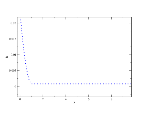
Figure 3: Initial state.

For the given $U=7.917e-4\,\mbox{m/s}$ and $R$ we find the angular velocity $\Omega=U/R=0.02908\mbox{s}^{-1}=0.277\,\mbox{r.p.m}$, where the last equality is obtained by multiplying with $60/2\pi$. For these values the capillary number is small $\mbox{Ca}=0.01089$, the length scales are $\tilde{H}=\tilde{L}=l_{\mathrm{cap}}=(\sigma/\rho g)^{1/2}=2.723e-3\mbox{m}$, $\hat{\Omega}=1.089e-3$ and the dimensionless radius of the disk is $10$. The resulting steady state is shown on the top of figure 3. It shows the an increase of thickness as the radius and hence the angular velocity increases, as expected. With increasing $\theta$ gravity causes the film to move downwards resulting in a ridge of fluid, that thickens with increasing $\theta$ and reenters the bath with a typical capillary ridge. If we increase $\Omega$, while keeping the other dimensional parameters and disk radius fixed, neither the length scales nor the dimensionless radius of the disk change, but $U$, the capillary number and $\hat{\Omega}$ do. As examples we let

$$\Omega=1.0\quad\mbox{rpm}: U=0.2851e-2\quad\mbox{m/s},\quad\mbox{Ca}=0.03922,\quad\hat{\Omega}=3.922e-3,$$

$$\Omega=2.0\quad\mbox{rpm}: U=0.5703e-2\quad\mbox{m/s},\quad\mbox{Ca}=0.07845,\quad\hat{\Omega}=7.843e-3,$$

Figure 4 illustrates the steady states for rotation velocities $\Omega=0.277$, $1.0$, $2.0$ r.p.m. from top to bottom, respectively. In all cases the height of the film in the figures is multiplied by the factor of $10$ to contrast more clearly the structure of the film patterns.

One observes for all values of $\Omega$ of the steady solutions a region of liquid drag-out with a meniscus profile and a drag-in region with a capillary wave on the opposite side of the axis. Such an oscillation of the height is typically found for the reverse Landau-Levich problem when a liquid thin film is dragged into a liquid bath, see for example [2, 7, 16, 19]. It can be seen more clearly when comparing the cross sections of the liquid profiles at constant radii. In figure 5 we compare for the radius $r=9$ the cross section for $\Omega=0.277$, $1.0$, $2.0$, $3.0\,$ r.p.m. (Note, that here as further below, values such as for $r$ without an explicit dimensions are in fact dimensionless). The figure also shows that the the average liquid height increases when $\Omega$ increases.

These results are qualitatively in accordance with the problem for the drag-out and drag-in cases. We will further investigate the quantitative comparison.

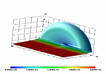
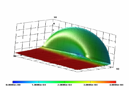
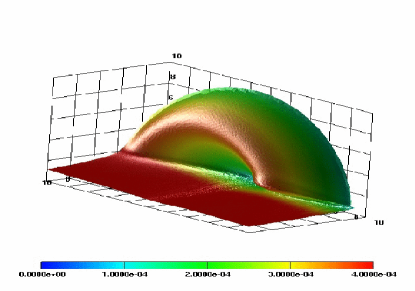
Figure 4: Steady solutions at $\Omega=0.277,1.0,2.0\,$ r.p.m.

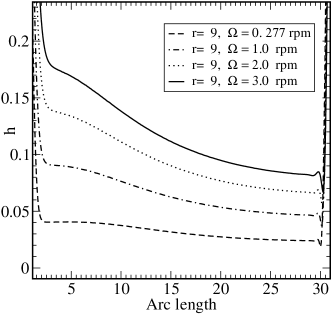
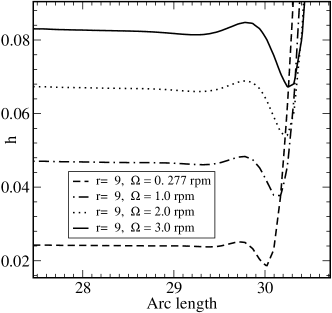
Figure 5: Comparisons of the profiles of the cross sections for the film profile for radius $r=9$. On the right hand side where the film is pulled into the bath a capillary wave is formed. This region is enlarged on the right figure. Note, “Arc length” denotes $r\theta$.

4.1.2 Comparison with the drag-out problem

Asymptotic estimate of the film thickness

We now derive an asymptotic approximation of the film thickness using a one dimensional approximation based on the results of Landau, Levich [9] and Wilson [18] for the planar-symmetric case.

For our comparisons we focus on the case where the disk is half immersed, i.e. $a=0$. Then, if we only retain the axial components in the stationary form of (2.44), and after substituting $r\theta\mapsto y$, $rd\theta\mapsto dy$ we obtain the equation

$$\frac{d}{dy}\left[\frac{h^{3}}{3}(p_{y}+1)-\hat{\Omega}rh\right]=0,$$ (4.1)

with

$$p=-\frac{d}{dy}\frac{h_{y}}{(1+h_{y}^{2})^{1/2}}.$$ (4.2)

Boundary conditions are

$$\lim_{y\rightarrow\infty}h=h_{\infty},\qquad\lim_{y\rightarrow 0}h=\infty,\quad\lim_{y\rightarrow 0}p=0.$$ (4.3)

Integrating (4.1), (4.2) once and using the boundary conditions (4.3) yields

$$h^{3}\frac{d^{2}}{dy^{2}}\frac{h_{y}}{(1+h_{y}^{2})^{1/2}}=-3r\hat{\Omega}(h-h_{\infty})+(h^{3}-h_{\infty}^{3}).$$ (4.4)

We rescale this equation to bring it into the form

$$h=(r\hat{\Omega})^{1/2}\bar{h},\quad h_{\infty}=(r\hat{\Omega})^{1/2}\bar{h}_{\infty},\quad y=(r\hat{\Omega})^{1/6}\bar{y},$$ (4.5)

to get

$$\bar{h}^{3}\frac{d^{2}}{d\bar{y}^{2}}\frac{\bar{h}_{\bar{y}}}{\left(1+(r\hat{\Omega})^{2/3}{\bar{h}}_{\bar{y}}^{2}\right)^{1/2}}=-3(\bar{h}-\bar{h}_{\infty})+(\bar{h}^{3}-\bar{h}_{\infty}^{3}).$$ (4.6)

For this equation, Wilson’s formula [18] gives the asymptotic approximation for the film thickness

$$\bar{h}_{\infty}=0.94581\,(r\hat{\Omega})^{1/6},$$

i.e. from (4.5),

$$h_{\infty}=0.94581\,(r\hat{\Omega})^{2/3}.$$ (4.7)

Figure 6 shows $h_{\infty}$ as a function of $r\hat{\Omega}$. Good agreement of the one-dimensional numerical results with the corresponding higher order asymptotic formula is achieved for small values of $r\hat{\Omega}$.

The meniscus profile $h(y)$ in figure 7 is now computed for the values given in section (4.1.1). Recall that $\hat{\Omega}=1.089e-3.$ At $r=9$, we have $r\hat{\Omega}=0.009801$, hence, from (4.7), $h_{\infty}=0.0433$.

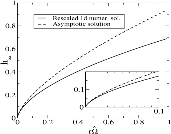
Figure 6: Comparison of numerical results for the one-dimensional problem (4.4) with the asymptotic formula for $h_{\infty}$ versus $r\hat{\Omega}$, (4.7).

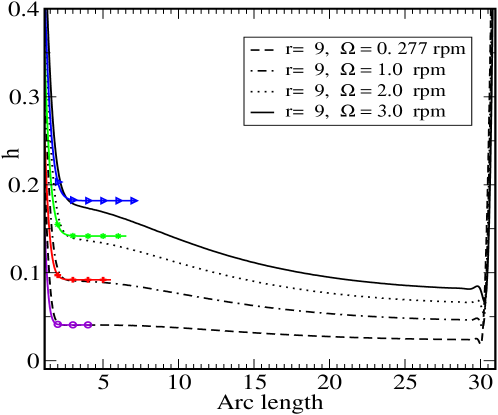
Figure 7: Meniscus profiles computed with the 1D model (4.4) (curves with symbols), for $\Omega=0.277\,({\rm circles}),1.0\,({\rm stars}),2.0\,({\rm plusses}),3.0\,({\rm triangles})$, and comparison with the profiles obtained for the cross section of the film profile for the rotating disk. “Arc length” denotes $r\theta$.

We now compare the meniscus profile computed with (4.6) for the drag-out problem with the numerical solution for the steady state of our problem (2.44)–(2.48). For this we take results for the cross section along constant radii. In figure 6 we performed the comparison for the cross section for the height profile at radius $r=9$, for $0\leq\theta\leq 180$, i.e. from the point where the film is dragged out to the point where it reenters the liquid bath. We see that there is excellent quantitative agreement in the vicinity of the meniscus region as it enters the thin film region.

4.1.3 Comparison with the hyperbolic regime

Further out into the disk region the height profile will deviate from the height obtained for the drag-out problem. There the variation of the height along the directions parallel to the disk is very small, which is clearly seen in our numerical simulations, so that surface tension will play a negligible role.

Starting from equation (2.44) we consider the steady state problem

$$\frac{\partial}{\partial r}\left[r\frac{h^{3}}{3}\sin\theta\right]+\frac{\partial}{\partial\theta}\left[\frac{h^{3}}{3}\cos\theta-\hat{\Omega}rh\right]=0,$$ (4.8)

to describe the dynamics far away from the meniscus. This can be simplified to the hyperbolic equation

$$h^{2}r\sin\theta\frac{\partial h}{\partial r}+\left(h^{2}\cos\theta-\hat{\Omega}r\right)\frac{\partial h}{\partial\theta}=0$$ (4.9)

Using the method of characteristics, this problem can be solved in form of an intitial value problem for the system of the coupled ordinary differential equations

$$\frac{dr}{d\tau} = h^{2}(r_{0},0)\,r\sin\theta,\qquad r(0)=r_{0}$$ (4.10a)

$$\frac{d\theta}{d\tau} = h^{2}(r_{0},0)\cos\theta-\hat{\Omega}r,\qquad\theta(0)=0$$ (4.10b)

Using as the initial condition the height found from (4.6) or simply by making use of formula (4.7) for a chosen $r_{0}$ we can integrate (4.10a), (4.10b) to obtain characteristics. This is shown in figure 8 for $\Omega=0.277$ as an example. The results are similar for the other angular velocities. As can be seen, the comparison of the characteristics that start from the meniscus region shows good agreement with the contour lines found from the FEM computation. Note, that the contour lines that start at the boundary of the rotating disk strongly depend on the conditions there.

Interestingly, one can get a good idea on the film profile as a function of the angular velocity $\hat{\Omega}$ by simply solving (4.10a), (4.10b) for $r$ as a function of $\theta$ directly by taking

$$\frac{dr/d\tau}{d\theta/d\tau}=\frac{dr}{d\theta}=\frac{r\sin\theta}{\cos\theta-\hat{\Omega}r/h_{0}^{2}},$$ (4.11)

which can be solved to yield

$$r(\theta)=\frac{h_{0}^{2}}{\hat{\Omega}}\left(\cos\theta\pm\sqrt{\cos^{2}\theta-2c_{0}\frac{\hat{\Omega}}{h_{0}^{2}}}\right),$$ (4.12)

where the integration constant is

$$c_{0}=r(0)\cos\theta(0)-\frac{\hat{\Omega}r^{2}(0)}{2h^{2}_{0}}.$$ (4.13)

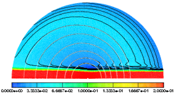
Figure 8: Comparison of contour lines from our FEM computation (black curves) for $\Omega=0.277$ with the characteristics (white curves) for $r_{0}=1.962,2.670,3.560,4.572,5.759,6.877$ and corresponding heights of $h_{0}=0.0130,0.0182,0.0234,0.0286,0.0338,0.0390$, respectively. Note, the corresponding 3D plot in figure 4.

4.2 Film patterns for slightly immersed disks

When the disk is half-immersed (immersion height $a=0$) the film thickness above the drag-out region will be renewed with every rotation and can be described by the classic drag-out problem. Furthermore, the film profile is slightly deformed by the effects of gravity before being drawn into the liquid bath accompanied by a typical oscillation in the thicknes of the film. The simple pattern emerging from this configuration changes when the immersion height is $a$ is increased.

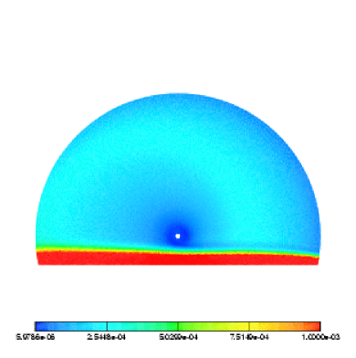
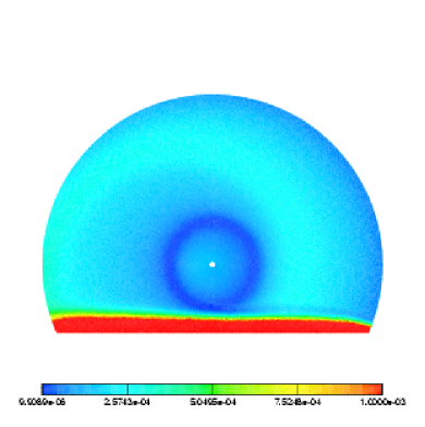
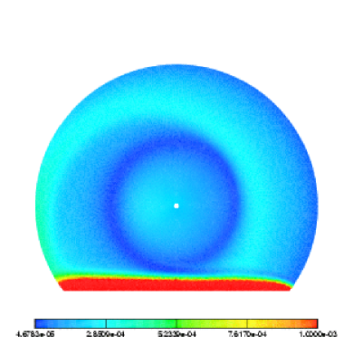
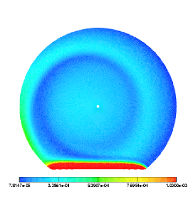
Figure 9: Steady solution at $\Omega=1$  r.p.m. for immersion depth of $a=0.2,0.4,0.6,0.8$

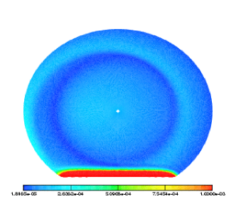
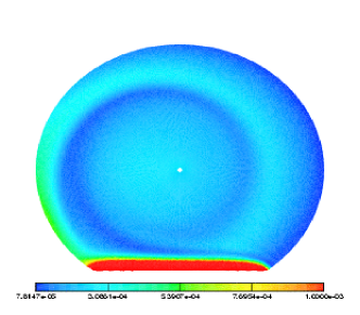
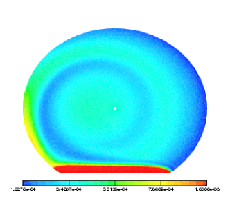
Figure 10: Steady solution for immersion depth of $a=0.8$ at angular velocity $\Omega=0.277,1.0,2.0$  r.p.m.

So in the final part of the paper we are interested in the new patterns that emerge when changing the two parameters $a$ and $\Omega$.

In the following figures 9 we first show the effect of varying the immersion depth from $a=0.2$ to $a=0.8$, leaving all other parameters as in the case of the half-immersed disk with $\Omega=1.0$. We observe an emerging almost symmetrical circular region where the film height has a minimum. This radius of the circular region increases with the immersion depth $a$. In fact, the radius quite closely corresponds to the distance from the minimum of the drag-in capillary wave to the vertical height of the rotation axis ($a=0$, see figure 1). By adjusting $a$ one can therfore achieve thin and fairly constant film profiles.

When the angular velocity is increased, not only does the fluid volume on the disk increase but the circular region is shifted towards the left, where the film is dragged out. This is demonstrated in figure 10 for the case of the immersion height $a=0.8$. To see this effect more clearly we compare horizontal cross sections at $r=0$ for the film thickness, shown in figure 11.

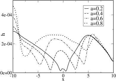
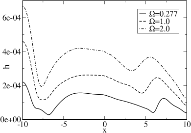
Figure 11: Horizontal cross sections through $r=0$ for the film thickness as the immersion depth is increased (left) and as the angular velocity inincreased (right)

5 Conclusions

In this work we have derived a dimension-reduced generalized lubrication model for the problem of the fully three-dimensional free-boundary problem for the vertically rotating disk, dragging out a thin film from a liquid bath. The resulting two-dimensional nonlinear degenerate fourth-order boundary value problem was solved numerically using a finite element scheme. For the steady state solutions we performed an asymptotic analysis near the meniscus region and a careful comparison with cross sections of the numerical solutions along constant radii gave good agreement. Away from the liquid bath we could show good agreement of our numerical solution with analytic solutions of the corresponding hyperbolic problem.

For slightly immersed disks we observed patterns for the film profile on the disk, which we studied as a function of the immersion depth and the angular velocity. Interestingly, the dependence of surface area of the film profile and of the volume fluid dragged out is not trivial. Of course we only touched upon the rich structure of possible patterns and outlined some general tendencies. More detailed systematic study is subject of current research. It is now possible to find optimum configurations that will be of importance for various technological and industrial applications. For example, in PET-reactors the fluid mechanical problem is coupled to chemical reactions taking place mainly on the film surface, so that here it is important to obtain thin films with high surface area.

References

- Christodoulou et al. [1990] M. S. Christodoulou, J. T. Turner, and S.D.R. Wilson. A model for the low to modererate speed performance of the rotating disk skimmer. J. Fluids Engr., 112:476–480, 1990.
- Cook and Clark [1973] R. A. Cook and R. H. Clark. An analysis of the stagnant band on falling liquid films. Ind. Engr. Chem. Fundam., 12:106–114, 1973.
- Davis and Duff [1997] T. A. Davis and I. S. Duff. An unsymmetric-pattern multifrontal method for sparse lu factorization. SIAM J. Matrix Analysis and Applications, 19:140–158, 1997.
- Emslie et al. [1958] A.G. Emslie, F.T. Bonner, and L.G. Peck. Flow of a viscous liquid on a rotating disk. J. Appl. Phys., 29:858–862, 1958.
- Fraysse and Homsy [1994] N. Fraysse and G.M. Homsy. An experimental study of rivulet instabilites in centrifugal spin coating of viscous newtonian and non-newtonian fluids. Phys. Fluids, 6:1491–1504, 1994.
- H.R.Schwarz [1991] H.R.Schwarz. Methode der finiten elemente. Teubner Studienbücher, Stuttgart, 1991.
- H.S.Keshgi et al. [1992] H.S.Keshgi, S.F. Kistler, and L.E. Scriven. Rising and falling film flows: viewed from a first order approximation. Chem. Engr. Sci., 47:683–694, 1992.
- Institute [2005] Bioengineering Institute. Fem/bem notes. The Univeersity of Auckland, New Zealand, 2005.
- Landau and Levich [1942] L. Landau and B. Levich. Dragging of a liquid by a moving plate. Acta Physicochimica U.R.S.S., 17:42–54, 1942.
- Münch [2002] A. Münch. The thickness of a Marangoni-driven thin liquid film emerging from a meniscus. SIAM J. Appl. Math, 62(6):2045–2063, 2002.
- Myers and Charpin [2001] T. G. Myers and J. P. F. Charpin. The effect of the coriolis force on axisymmetric rotating thin film flows. International Journal of Non-Linear Mechanics, 36:629–635, 2001.
- Myers and Lombe [2006] T. G. Myers and M. Lombe. The importance of the Coriolis force on axisymmetric horizontal rotating thin film flows. Chem. Engineering and Processing, 45:90–98, 2006.
- Ozar at al. [2003] B. Ozar and B.M. Cetegen and A. Faghri. Experiments on the flow of a thin liquid film over a horizontal stationary and rotating disk surface. Experiments in Fluids, 34:556–565, 2003.
- Reinelt [1995] R. Reinelt. Delaunay gittergenerator. Technischer Bericht, Hermann-Föttinger-Institut, TU Berlin, 1995.
- Reisfeld et al. [1991] B. Reisfeld, S. G. Bankoff, and S. H. Davis. The dynamics and stability of thin liquid films during spin coating. i. films with constant rates of evaporation or absorption. J. Appl. Phys., 70:5258–5266, 1991.
- Ruschak [1978] K. J. Ruschak. Flow of a falling film into a pool. A. I. Ch. E. J., 24:705–709, 1978.
- Schwartz [2001] L.W. Schwartz. On the asymptotic analysis of surface-stress-driven thin-layer flow. J. Engr. Math., 39:171–188, 2001.
- Wilson [1982] S.D.R. Wilson. The drag-out problem in film coating theory. J. Engr. Math., 16:209–221, 1982.
- Wilson and Jones [1982] S.D.R. Wilson and A.F. Jones. The entry of a falling film into a pool and the air-entrainment problem. J. Fluid. Mech., 128:219–230, 1982.