Consequences of Symmetries on the Analysis and Construction of Turbulence Models

Consequences of Symmetries on the Analysis
and Construction of Turbulence Models

Dina RAZAFINDRALANDY and Aziz HAMDOUNI

D. Razfindralandy and A. Hamdouni

LEPTAB, Avenue Michel Crépeau, 17042 La Rochelle Cedex 01, France drazafin@univ-lr.fr, ahamdoun@univ-lr.fr

Received October 28, 2005, in final form May 02, 2006; Published online May 12, 2006

Since they represent fundamental physical properties in turbulence (conservation laws, wall laws, Kolmogorov energy spectrum, …), symmetries are used to analyse common turbulence models. A class of symmetry preserving turbulence models is proposed. This class is refined such that the models respect the second law of thermodynamics. Finally, an example of model belonging to the class is numerically tested.

turbulence; large-eddy simulation; Lie symmetries; Noether’s theorem; thermodynamics

22E70; 35A30; 35Q30; 76D05; 76F65; 76M60

1 Introduction

Turbulence is one of the most interesting research fields in mechanics. But with the current performance of computers, a direct simulation of a turbulent flow remains difficult, even impossible in many cases, due to the high computational cost that it requires. To reduce this computational cost, use of turbulence models is necessary. At the present time, many turbulence models exist (see [22]). However, derivation of a very large majority of them does not take into account the symmetry group of the basic equations, the Navier–Stokes equations.

In turbulence, symmetries play a fundamental role in the description of the physics of the flow. They reflect existence of conservation laws, via Noether’s theorem. Notice that, even if Navier–Stokes equations are not directly derived from a Lagrangian, Noether’s theorem can be applied and conservation laws can be deduced. Indeed, there exists a Lagrangian (which will be called “bi-Lagrangian” here) from which Navier–Stokes equations, associated to their “adjoint” equations, can be derived. A way in which this bi-Lagrangian can be calculated is described by Atherton and Homsy in [1]. The expression of this bi-Lagrangian and the infinitesimal generators of the associated Euler–Lagrange equations are given in Appendix A. However, the conservation laws are not studied in this paper.

The importance of symmetries in turbulence is not limited to the derivation of conservation laws. Ünal also used a symmetry approach to show that Navier–Stokes equations may have solutions which have the Kolmogorov form of the energy spectrum [24]. Next, symmetries enabled Oberlack to derive some scaling laws for the velocity and the two point correlations [19]. Some of these scaling laws was reused by Lindgren et al in [15] and are proved to be in good agreement with experimental data. Next, symmetries allowed Fushchych and Popowych to obtain analytical solutions of Navier–Stokes equations [8]. The study of self-similar solutions gives also an information on the behaviour of the flow at a large time [4]. Lastly, we mention that use of discretisation schemes which are compatible with the symmetries of an equation reduces the numerical errors [20, 13].

Introduction of a turbulence model in Navier–Stokes equations may destroy symmetry properties of the equations. In this case, physical properties (conservation laws, scaling laws, spectral properties, large-time behaviour, …) may be lost. In order to represent the flow correctly, turbulence models should then preserve the symmetries of Navier–Stokes equations. The first aim of this paper is to show that most of the commonly used subgrid turbulence models do not have this property. The second goal is to present a new way of deriving models which are compatible with the symmetries of Navier–Stokes equations and which, unlike many existing models, conform to the second law of thermodynamics. As it will be shown in appendix, conformity with this law leads to stability of the model, in the sense of $L^{2}$.

The paper will be structured as follows. In Section 2, the principle of turbulence modelling, using the large-eddy simulation approach, will be concisely presented, as well as some common models. These models will be analysed in Section 3 under the symmetry consideration. In Section 4, a class of symmetry preserving and thermodynamically consistent models are derived. One example of a model of the class is numerically tested in Section 5. Some conclusions will be drawn in Section 6. In Appendix A, it will be shown that Navier–Stokes equations can be derived from a bi-Lagrangian. At last, in Appendix B, stability of thermodynamically consistent models is proved.

2 Large-eddy simulation

Consider a three-dimensional incompressible Newtonian fluid, with density $\rho$ and kinematic viscosity $\nu$. The motion of this fluid is governed by Navier–Stokes equations:

$$\cfrac{\partial\boldsymbol{u}}{\partial t}\,+\operatorname{div}(\boldsymbol{u}\otimes\boldsymbol{u})+\cfrac{1}{\rho}\,\nabla p=\operatorname{div}\mathsfb{T},$$

$$\operatorname{div}\boldsymbol{u}=0,$$ (1)

where $\boldsymbol{u}=(u_{i})_{i=1,2,3}$ and $p$ are respectively velocity and pressure fields and $t$ the time variable. $\mathsfb{T}$ is a tensor such that $\rho\mathsfb{T}$ is the viscous constraint tensor. $\mathsfb{T}$ can be linked to the strain rate tensor ${\mathsfb{S}=(\nabla\boldsymbol{u}+{\,{}^{\scriptscriptstyle T}}\nabla\boldsymbol{u})/2}$ according to the relation:

$$\mathsfb{T}=\cfrac{\partial\psi}{\partial\mathsfb{S}}\,,$$

$\psi$ being a positive and convex “potential” defined by:

$$\psi=\nu\operatorname{tr}\mathsfb{S}^{2}.$$

Since a direct numerical simulation of a realistic fluid flow requires very significant computational cost, (1) is not directly resolved. To circumvent the problem, some methods exist. The most promising one is the large-eddy simulation. It consists in representing only the large scales of the flow. Small scales are dropped from the simulation; however, their effects on the large scales are taken into account. This enables to take a much coarser grid.

Mathematically, dropping small scales means applying a low-pass filter. The large or resolved scales $\overline{\phi}$ of a quantity $\phi$ are defined by the convolution:

$$\overline{\phi}=G_{\overline{\delta}}*\phi,$$

where $G_{\overline{\delta}}$ is the filter kernel with a width $\overline{\delta}$, and the small scales $\phi^{\prime}$ are defined by

$$\phi^{\prime}=\phi-\overline{\phi}.$$

It is required that the integral of $G_{\overline{\delta}}$ over $\mathbb{R}^{3}$ is equal to 1, such that a constant remains unchanged when the filter is applied.

In practice, $(\overline{\boldsymbol{u}},\overline{p})$ is directly used as an approximation of $(\boldsymbol{u},p)$. To obtain $(\overline{\boldsymbol{u}},\overline{p})$, the filter is applied to (1). If the filter is assumed to commute with the derivative operators (that is not always the case in a bounded domain), this leads to:

$$\cfrac{\partial\overline{\boldsymbol{u}}}{\partial t}\,+\operatorname{div}(\overline{\boldsymbol{u}}\otimes\overline{\boldsymbol{u}})+\cfrac{1}{\rho}\nabla\overline{p}=\operatorname{div}(\overline{\mathsfb{T}}+\mathsfb{T}_{s}),$$

$$\operatorname{div}\overline{u}=0,$$ (2)

where $\mathsfb{T}_{s}$ is the subgrid stress tensor defined by $\mathsfb{T}_{s}=\overline{\boldsymbol{u}}\otimes\overline{\boldsymbol{u}}-\overline{\boldsymbol{u}\otimes\boldsymbol{u}}$ which must be modelled (expressed by a function of the resolved quantities) to close the equations. Currently, an important number of models exists. Some of the most common ones will be reminded here. They will be classified in four categories: turbulent viscosity, gradient-type, similarity-type and Lund–Novikov-type models.

2.1 Turbulent viscosity models

Turbulent viscosity models are models which can be written in the following form:

$$\mathsfb{T}_{s}^{d}=\nu_{s}\overline{\mathsfb{S}},$$ (3)

where $\nu_{s}$ is the turbulent viscosity. The superscript (^d) represents the deviatoric part of a tensor:

$$\mathsfb{Q}\ \mapsto\ \mathsfb{Q}^{d}=\mathsfb{Q}-\cfrac{1}{3}(\operatorname{tr}\mathsfb{Q})\mathsfb{I_{d}},$$

where $\mathsfb{I_{d}}$ is the identity operator. The deviatoric part has been introduced in order to have the equality of the traces in (3). In what follows, some examples of turbulent viscosity models are presented.

• Smagorinsky model (see [22]) is one of the most widely used models. It uses the local equilibrium hypothesis for the calculation of the turbulent viscosity. It has the following expression:

  $$\mathsfb{T}_{s}^{d}=(C_{S}\overline{\delta})^{2}|\overline{\mathsfb{S}}|\overline{\mathsfb{S}},$$

  where $C_{S}\simeq 0.148$ is the Smagorinsky constant, $\overline{\delta}$ the filter width and $|\overline{\mathsfb{S}}|=\sqrt{2\operatorname{tr}\big{(}\overline{\mathsfb{S}}^{2}\big{)}}$.

• In order to reduce the modelling error of Smagorinsky model, Lilly [14] proposes a dynamic evaluation of the constant $C_{S}$ by a least-square approach. This leads to the so-called dynamic model defined by:

  $$\mathsfb{T}^{d}_{s}=C_{d}\overline{\delta}^{2}|\overline{\mathsfb{S}}|\overline{\mathsfb{S}},\qquad\text{with}\quad C_{d}=\cfrac{\operatorname{tr}(\mathsfb{LM})}{\operatorname{tr}\mathsfb{M}^{2}}.$$ (4)

  In these terms,

  $$\mathsfb{L}=\widetilde{\overline{\boldsymbol{u}}}\otimes\widetilde{\overline{\boldsymbol{u}}}-\widetilde{\overline{\boldsymbol{u}}\otimes\overline{\boldsymbol{u}}},\qquad\mathsfb{M}=\overline{\delta}^{2}\widetilde{|\overline{\mathsfb{S}}|\overline{\mathsfb{S}}}-\widetilde{\overline{\delta}}^{2}|\widetilde{\overline{\mathsfb{S}}}|\widetilde{\overline{\mathsfb{S}}},$$

  the tilde represents a test filter whose width is $\widetilde{\overline{\delta}}$, with $\widetilde{\overline{\delta}}>\overline{\delta}$.

  The last turbulent viscosity model which will be considered is the structure function model.

• Metais and Lesieur [16] make the hypothesis that the turbulent viscosity depends on the energy at the cutoff. Knowing its relation with the energy density in Fourier space, they use the second order structure function and propose the structure function model:

  $$\mathsfb{T}_{s}^{d}=C_{SF}\overline{\delta}\sqrt{\overline{F}_{2}(\overline{\delta}})\,\overline{\mathsfb{S}},$$ (5)

  where $\overline{F}_{2}$ is the spatial average of the filtered structure function:

  $$r\ \mapsto\ \overline{F}_{2}(r)=\iint_{\|\boldsymbol{z}\|=r}\|\overline{\boldsymbol{u}}(\boldsymbol{x})-\overline{\boldsymbol{u}}(\boldsymbol{x}+\boldsymbol{z})\|^{2}\,\textrm{d}\boldsymbol{z}\,\textrm{d}\boldsymbol{x}.$$

The next category of models, which will be reminded, consists of the gradient-type models.

2.2 Gradient-type models

To establish the gradient-type models, the subgrid stress tensor is decomposed as follows:

$$\mathsfb{T}_{s}=\overline{\boldsymbol{u}}\otimes\overline{\boldsymbol{u}}-(\ \overline{\overline{\boldsymbol{u}}\otimes\overline{\boldsymbol{u}}}+\overline{\overline{\boldsymbol{u}}\otimes\boldsymbol{u}^{\prime}}+\overline{\boldsymbol{u}^{\prime}\otimes\overline{\boldsymbol{u}}}+\overline{\boldsymbol{u}^{\prime}\otimes\boldsymbol{u}^{\prime}}\ ).$$

Next, each term between the brackets are written in Fourier space. Then, the Fourier transform of the filter, which is assumed to be Gaussian, is approximated by an appropriate function. Finally, the inverse Fourier transform is computed. The models in this category differ by the way in which the Fourier transform of the filter is approximated.

• If a second order Taylor series expansions according to the filter width $\overline{\delta}$ is used in the approximation, one has:

  $$\mathsfb{T}_{s}=-\cfrac{\overline{\delta}^{2}}{12}\ \nabla\overline{\boldsymbol{u}}\ {\,{}^{\scriptscriptstyle T}}\nabla\overline{\boldsymbol{u}}.$$ (6)

• The gradient model is not dissipative enough and not numerically stable [26, 11]. Thus, it is generally combined to Smagorinsky model. This gives Taylor model:

  $$\mathsfb{T}_{s}=-\cfrac{\overline{\delta}^{2}}{12}\ \nabla\overline{\boldsymbol{u}}\ {\,{}^{\scriptscriptstyle T}}\nabla\overline{\boldsymbol{u}}+C\overline{\delta}^{2}|{\overline{\mathsfb{S}}}|\overline{\mathsfb{S}}.$$

• The Taylor approximation of the Fourier transform of the filter tends to accentuate the small frequencies rather than attenuating them. Instead, a rational approximation can be used [12, 2]. This gives the following expression of the model:

  $$\mathsfb{T}_{s}=-\cfrac{\overline{\delta}^{2}}{12}\left(\mathsfb{I_{d}}-\cfrac{\overline{\delta}^{2}}{24}\nabla^{2}\right)^{-1}[\nabla\overline{\boldsymbol{u}}\ {\,{}^{\scriptscriptstyle T}}\nabla\overline{\boldsymbol{u}}]+C\overline{\delta}^{2}|{\overline{\mathsfb{S}}}|\overline{\mathsfb{S}}.$$

  To avoid the inversion of the operator $\left(\mathsfb{I_{d}}-\frac{\overline{\delta}^{2}}{24}\nabla^{2}\right)$, $\mathsfb{T}_{s}$ is approximated by:

  $$\mathsfb{T}_{s}=-\cfrac{\overline{\delta}^{2}}{12}\ G_{\overline{\delta}}*[\nabla\overline{\boldsymbol{u}}\ {\,{}^{\scriptscriptstyle T}}\nabla\overline{\boldsymbol{u}}]+C\overline{\delta}^{2}|{\overline{\mathsfb{S}}}|\overline{\mathsfb{S}}.$$ (7)

  $G_{\overline{\delta}}$ is the kernel of the Gaussian filter. The convolution is done numerically. The model (7) is called the rational model.

2.3 Similarity-type models

Models of this category are based on the hypothesis that the statistic structure of the small scales are similar to the statistic structure of the smallest resolved scales. Separation of the resolved scales is done using a test filter (symbolized by $\widetilde{\phantom{x}}$). The largest resolved scales are then represented by $\widetilde{\overline{\boldsymbol{u}}}$ and the smallest ones by $\overline{\boldsymbol{u}}-\widetilde{\overline{\boldsymbol{u}}}$. From this hypothesis, we deduce the similarity model:

$$\mathsfb{T}_{s}=\widetilde{\overline{\boldsymbol{u}}}\otimes\widetilde{\overline{\boldsymbol{u}}}-\widetilde{\overline{\boldsymbol{u}}\otimes\overline{\boldsymbol{u}}}.$$ (8)

From this expression, many other models can be obtained by multiplying by a coefficient, by filtering again the whole expression or by mixing with a Smagorinsky-type model.

The last models that we will consider are Lund–Novikov-type models.

2.4 Lund–Novikov-type models

• Lund and Novikov include the filtered vorticity tensor $\mathsfb{\overline{W}}=(\nabla\overline{\boldsymbol{u}}-{\,{}^{\scriptscriptstyle T}}\nabla\overline{\boldsymbol{u}})$ in the expression of the subgrid model. Cayley–Hamilton theorem gives then the Lund–Novikov model (see [22]):

  $$-\mathsfb{T}_{s}^{d}=C_{1}\overline{\delta}^{2}|\overline{\mathsfb{S}}|\overline{\mathsfb{S}}+C_{2}\overline{\delta}^{2}(\overline{\mathsfb{S}}^{2})^{d}+C_{3}\overline{\delta}^{2}\big{(}\mathsfb{\overline{W}}^{2}\big{)}^{d}$$

  $$\phantom{-\mathsfb{T}_{s}^{d}=}{}+C_{4}\overline{\delta}^{2}(\overline{\mathsfb{S}}\,\mathsfb{\overline{W}}-\mathsfb{\overline{W}}\,\overline{\mathsfb{S}})+C_{5}\overline{\delta}^{2}\cfrac{1}{|\overline{\mathsfb{S}}|}\big{(}\overline{\mathsfb{S}}^{2}\mathsfb{\overline{W}}-\overline{\mathsfb{S}}\,\mathsfb{\overline{W}}^{2}\big{)},$$ (9)

  where the coefficients $C_{i}$ depend on the invariants obtained from $\overline{\mathsfb{S}}$ and $\mathsfb{\overline{W}}$. The expression of these coefficients are so complex that they are considered as constants and evaluated with statistic techniques.

• To reduce the computation cost of the previous model, Kosovic brings a simplification and proposes the following model:

  $$-\mathsfb{T}_{s}^{d}=(C\overline{\delta})^{2}\left[2|\overline{\mathsfb{S}}|\overline{\mathsfb{S}}+C_{1}\big{(}\overline{\mathsfb{S}}^{2}\big{)}^{d}+C_{2}(\overline{\mathsfb{S}}\,\mathsfb{\overline{W}}-\mathsfb{\overline{W}}\,\overline{\mathsfb{S}})\right],$$ (10)

  where the constants $C$, $C_{1}$ and $C_{2}$ are calculated using the theory of homogeneous and isotropic turbulence.

The derivation of these models was done using different hypothesis but did not take into consideration the symmetries of Navier–Stokes equations which may then be destroyed. So, in the next section, these models will be analysed by a symmetry approach.

3 Model analysis

The (classical) symmetry groups of Navier–Stokes equations have been investigated for some decades (see for example [7, 3]). They are generated by the following transformations:

• The time translations: $(t,\boldsymbol{x},\boldsymbol{u},p)\mapsto(t+a,\boldsymbol{x},\boldsymbol{u},p)$,

• the pressure translations: $(t,\boldsymbol{x},\boldsymbol{u},p)\mapsto(t,\boldsymbol{x},\boldsymbol{u},p+\zeta(t))$,

• the rotations: $(t,\boldsymbol{x},\boldsymbol{u},p)\mapsto(t,\mathsfb{R}\boldsymbol{x},\mathsfb{R}\boldsymbol{u},p)$,

• the generalized Galilean transformations:

  $(t,\boldsymbol{x},\boldsymbol{u},p)\mapsto\left(t,\boldsymbol{x}+\boldsymbol{\alpha}(t),\boldsymbol{u}+\dot{\boldsymbol{\alpha}}(t),p-\rho\,\boldsymbol{x}\cdot\ddot{\boldsymbol{\alpha}}(t)\right)$,

• and the first scaling transformations: $(t,\boldsymbol{x},\boldsymbol{u},p)\mapsto(\mathrm{e}^{2a}t,\mathrm{e}^{a}\boldsymbol{x},\mathrm{e}^{-a}\boldsymbol{u},\mathrm{e}^{-2a}\,p)$.

In these expressions, $a$ is a scalar, $\zeta$ (respectively $\boldsymbol{\alpha}$) a scalar (resp. vectorial) arbitrary function of $t$ and $\mathsfb{R}$ a rotation matrix, i.e. $\mathsfb{R}{\,{}^{\scriptscriptstyle T}}\mathsfb{R}=\mathsfb{I_{d}}$ and $\det\mathsfb{R}=1$. The central dot ($\cdot$) stands for $\mathbb{R}^{3}$ scalar product.

If it is considered that $\nu$ can change during the transformation (which is then an equivalence transformation [9]), one has the second scaling transformations:

$$(t,\boldsymbol{x},\boldsymbol{u},p,\nu)\mapsto(t,e^{a}\boldsymbol{x},e^{a}\boldsymbol{u},e^{2a}p,e^{2a}\nu),$$

where $a$ is the parameter.

Navier–Stokes equations admit other known symmetries which do not constitute a one-parameter symmetry group. They are

• the reflections: $(t,\boldsymbol{x},\boldsymbol{u},p)\mapsto(t,\mathsfb{\Lambda}\boldsymbol{x},\mathsfb{\Lambda}\boldsymbol{u},p)$,

  which are discrete symmetries, $\mathsfb{\Lambda}$ being a diagonal matrix $\mathsfb{\Lambda}=\text{diag}(\iota_{1},\iota_{2},\iota_{3})$ with $\iota_{i}=\pm 1,\ \ i=1,2,3$,

• and the material indifference: $(t,\boldsymbol{x},\boldsymbol{u},p)\mapsto(t,\widehat{\boldsymbol{x}},\widehat{\boldsymbol{u}},\widehat{p})$,

  in the limit of a 2D flow in a simply connected domain [5], with

  $$\widehat{\boldsymbol{x}}=\mathsfb{R}(t)\ \boldsymbol{x},\qquad\widehat{\boldsymbol{u}}=\mathsfb{R}(t)\;\boldsymbol{u}+\dot{\mathsfb{R}}(t)\;\boldsymbol{x},\qquad\widehat{p}=p-3\omega\varphi+\cfrac{1}{2}\omega^{2}\|\boldsymbol{x}\|^{2},$$

  where $\mathsfb{R}(t)$ is a 2D rotation matrix with angle $\omega t$, $\omega$ an arbitrary real constant, $\varphi$ the usual 2D stream function defined by:

  $$\boldsymbol{u}=\mathrm{curl}(\varphi\boldsymbol{e}_{3}),$$

  $\boldsymbol{e}_{3}$ the unit vector perpendicular to the plane of the flow and $\|{\scriptscriptstyle\bullet}\|$ the Euclidean norm.

We wish to analyse which of the models cited above is compatible with these symmetries. The set of solutions $(\boldsymbol{u},p)$ of Navier–Stokes equations (1) is preserved by each of the symmetries. We then require that the set of solutions $(\overline{\boldsymbol{u}},\overline{p})$ of the filtered equations (2) is also preserved by all of these transformations, since $(\overline{\boldsymbol{u}},\overline{p})$ is expected to be a good approximation of $(\boldsymbol{u},p)$. More clearly, if a transformation

$$T\ :\ (t,x,\boldsymbol{u},p)\mapsto(\widehat{t},\widehat{x},\widehat{u},\widehat{p})$$

is a symmetry of (1), we require that the model is such that the same transformation, applied to the filtered quantities:

$$T:(t,x,\overline{\boldsymbol{u}},\overline{p})\mapsto(\widehat{t},\widehat{x},\widehat{\overline{\boldsymbol{u}}},\widehat{\overline{p}}),$$

is a symmetry of the filtered equations (2). When this condition holds, the model will be said invariant under the relevant symmetry.

The filtered equations (2) may have other symmetries but with the above requirement, we may expect to preserve certain properties of Navier–Stokes equations (conservation laws, wall laws, exact solutions, spectra properties, …) when approximating $(\boldsymbol{u},p)$ by $(\overline{\boldsymbol{u}},\overline{p})$.

We will use the hypothesis that test filters do not destroy symmetry properties, i.e. $\widehat{\widetilde{\phi}}=\widetilde{\widehat{\phi}}$ for any quantity $\phi$.

For the analysis, the symmetries of (1) will be grouped into four categories:

• translations, containing time translations, pressure translations and the generalized Galilean transformations,

• rotations and reflections,

• scaling transformations,

• material indifference.

The aim is to search which models are invariant under the symmetries within the considered category.

3.1 Invariance under translations

Since almost all existing models are autonomous in time and pressure, the filtered equations (2) remain unchanged when a time or pressure translation is applied. Almost all models are then invariant under the time and the pressure translations.

The generalized Galilean transformations, applied to the filtered variables, have the following form:

$$(t,\boldsymbol{x},\overline{\boldsymbol{u}},\overline{p})\ \mapsto\ (\widehat{t},\widehat{x},\widehat{\overline{\boldsymbol{u}}},\widehat{\overline{p}})=\left(t,\boldsymbol{x}+\boldsymbol{\alpha}(t),\overline{\boldsymbol{u}}+\dot{\boldsymbol{\alpha}}(t),\overline{p}-\rho\,\boldsymbol{x}\boldsymbol{\cdot}\ddot{\boldsymbol{\alpha}}(t)\right).$$

All models in Section 2, in which $\boldsymbol{x}$ and $\overline{\boldsymbol{u}}$ are present only through $\nabla\overline{\boldsymbol{u}}$ are invariant since

$$\widehat{\nabla}\widehat{\overline{\boldsymbol{u}}}=\nabla\widehat{\overline{\boldsymbol{u}}}=\nabla\overline{\boldsymbol{u}},$$

where $\widehat{\nabla}=(\partial/\partial\widehat{x}_{1},\partial/\partial\widehat{x}_{2},\partial/\partial\widehat{x}_{3}).$

The remaining models, i.e. the dynamic and the similarity models are also invariant because

$$\widetilde{\widehat{\overline{\boldsymbol{u}}}\otimes\widehat{\overline{\boldsymbol{u}}}}-\widetilde{\widehat{\overline{\boldsymbol{u}}}}\otimes\widetilde{\widehat{\overline{\boldsymbol{u}}}}=\widetilde{(\overline{\boldsymbol{u}}+\dot{\boldsymbol{\alpha}})\otimes(\overline{\boldsymbol{u}}+\dot{\boldsymbol{\alpha}})}-\widetilde{(\overline{\boldsymbol{u}}+\dot{\boldsymbol{\alpha}})}\otimes\widetilde{(\overline{\boldsymbol{u}}+\dot{\boldsymbol{\alpha}})}=\widetilde{\overline{\boldsymbol{u}}\otimes\overline{\boldsymbol{u}}}-\widetilde{\overline{\boldsymbol{u}}}\otimes\widetilde{\overline{\boldsymbol{u}}}.$$

3.2 Invariance under rotations and reflections

The rotations and the reflections can be put together in a transformation:

$$(t,\boldsymbol{x},\boldsymbol{u},p)\mapsto(t,\mathsfb{\Upsilon}\boldsymbol{x},\mathsfb{\Upsilon}\boldsymbol{u},p)$$

where $\mathsfb{\Upsilon}$ is a constant rotation or reflection matrix. This transformation, when applied to the filtered variables, is a symmetry of (2) if and only if

$$\widehat{\mathsfb{T}}_{s}=\mathsfb{\Upsilon}\ \mathsfb{T}_{s}{\,{}^{\scriptscriptstyle T}}\mathsfb{\Upsilon}.$$ (11)

Let us check if the models respect this condition.

• For Smagorinsky model, we have:

  $$\widehat{\nabla}\widehat{\overline{\boldsymbol{u}}}=[\nabla(\widehat{\overline{\boldsymbol{u}}})]{\,{}^{\scriptscriptstyle T}}\mathsfb{\Upsilon}=[\nabla(\mathsfb{\Upsilon}\overline{\boldsymbol{u}})]{\,{}^{\scriptscriptstyle T}}\mathsfb{\Upsilon}=\mathsfb{\Upsilon}[\nabla\overline{\boldsymbol{u}}]{\,{}^{\scriptscriptstyle T}}\mathsfb{\Upsilon}.$$ (12)

  This leads to the objectivity of $\overline{\mathsfb{S}}$:

  $$\widehat{\overline{\mathsfb{S}}}=\mathsfb{\Upsilon}\ \overline{\mathsfb{S}}\ {\,{}^{\scriptscriptstyle T}}\mathsfb{\Upsilon}.$$

  And since $|\widehat{\overline{\mathsfb{S}}}|=|\overline{\mathsfb{S}}|$, (11) is verified. Smagorinsky model is then invariant.

• For similarity model (8), one has:

  $$\widehat{\overline{\boldsymbol{u}}}\otimes\widehat{\overline{\boldsymbol{u}}}=(\mathsfb{\Upsilon}\overline{\boldsymbol{u}})\otimes(\mathsfb{\Upsilon}\overline{\boldsymbol{u}})=\mathsfb{\Upsilon}(\overline{\boldsymbol{u}}\otimes\overline{\boldsymbol{u}}){\,{}^{\scriptscriptstyle T}}\mathsfb{\Upsilon}.$$

  By means of these relations, invariance can easily been deduced.

• The same relations are sufficient to prove invariance of the dynamic model since the trace remains invariant under a change of orthonormal basis.

• The structure function model (5) is invariant because the function $\overline{F}_{2}$ is not altered under a rotation or a reflection.

• Relations (12) can be used again to prove invariance of each of the gradient-type models.

• Finally, since

  $$\widehat{\overline{\mathsfb{W}}}=\mathsfb{\Upsilon}\ \overline{\mathsfb{W}}\ {\,{}^{\scriptscriptstyle T}}\mathsfb{\Upsilon},$$

  Lund–Novikov-type models are also invariant.

Any model of Section 2 is then invariant under the rotations and the reflections.

3.3 Invariance under scaling transformations

The two scaling transformations can be gathered in a two-parameter transformation which, when applied to the filtered variables, have the following expression:

$$(t,\boldsymbol{x},\overline{\boldsymbol{u}},\overline{p},\nu)\ \mapsto\ \big{(}\mathrm{e}^{2a}t,\mathrm{e}^{ab}\boldsymbol{x},\mathrm{e}^{b-a}\overline{\boldsymbol{u}},\mathrm{e}^{2b-2a}\overline{p},\mathrm{e}^{2b}\nu\big{)}.$$

where $a$ and $b$ are the parameters. The first scaling transformations corresponds to the case $b=0$ and the second ones to the case $a=0$.

It can be checked that the filtered equations (2) are invariant under the two scaling transformations if and only if

$$\widehat{\mathsfb{T}}_{s}=\mathrm{e}^{2b-2a}\mathsfb{T}_{s}.$$ (13)

Since $\widehat{\overline{\mathsfb{S}}}=\mathrm{e}^{-2a}\overline{\mathsfb{S}}$, this condition is equivalent to:

$$\widehat{\nu}_{s}=\mathrm{e}^{2b}\nu_{s}$$ (14)

for a turbulent viscosity model.

• For Smagorinsky model, we have:

  $$\widehat{\nu}_{s}=C_{S}\overline{\delta}^{2}|\widehat{\overline{\mathsfb{S}}}|=\mathrm{e}^{-2a}C_{S}\overline{\delta}^{2}|\overline{\mathsfb{S}}|=\mathrm{e}^{-2a}\nu_{s}.$$

  Condition (14) is violated. The model is invariant neither under the first nor under the second scaling transformations. Note that the filter width $\overline{\delta}$ does not vary since it is an external scale length and has no functional dependence on the variables of the flow.

• The dynamic procedure used in (4) restores the scaling invariance. Indeed, it can be shown that:

  $$\widehat{C}_{d}=\mathrm{e}^{2b+2a}C_{d},$$

  that implies:

  $$\widehat{\nu}_{s}=\widehat{C}_{d}\overline{\delta}^{2}|\widehat{\overline{\mathsfb{S}}}|=\mathrm{e}^{2b}C_{d}\overline{\delta}^{2}|\overline{\mathsfb{S}}|=\mathrm{e}^{2b}\nu_{s}.$$

  The dynamic model is then invariant under the two scaling transformation.

• For the structure function model, we have:

  $$\widehat{\overline{F}}_{2}=\mathrm{e}^{b-a}\overline{F}_{2}$$

  and then

  $$\widehat{\nu}_{s}=\mathrm{e}^{b-a}\nu_{sm},$$

  that proves that the model is not invariant.

• Since

  $$\widehat{\nabla}\widehat{\overline{\boldsymbol{u}}}=\mathrm{e}^{2a}\nabla\overline{\boldsymbol{u}}$$

  the gradient model (6) violates (13), $\mathsfb{T}_{s}$ varying in the following way:

  $$\widehat{\mathsfb{T}}_{s}=\mathrm{e}^{4a}\mathsfb{T}_{s}.$$

  This also implies that none of the gradient-type models is invariant.

• It is straight forward to prove that the similarity model (8) verifies (13) and is invariant.

• At last, Lund–Novikov-type models are not invariant because they comprise a term similar to Smagorinsky model.

In fact, none of the models where the external length scale $\overline{\delta}$ appears explicitly is invariant under the scaling transformations. Note that the dynamic model, which is invariant under these transformations, can be written in the following form:

$$\mathsfb{T}_{s}^{d}=\cfrac{\operatorname{tr}(\mathsfb{LN})}{\operatorname{tr}(\mathsfb{N}^{2})}\ |\overline{\mathsfb{S}}|\overline{\mathsfb{S}},$$

where

$$\mathsfb{N}=\ \widetilde{|\overline{\mathsfb{S}}|\overline{\mathsfb{S}}}-(\widetilde{\overline{\delta}}/\overline{\delta})^{2}|\widetilde{\overline{\mathsfb{S}}}|\widetilde{\overline{\mathsfb{S}}}.$$

It is then the ratio $\widehat{\overline{\delta}}/\overline{\delta}$ which is present in the model but neither $\overline{\delta}$ alone nor $\widehat{\overline{\delta}}$ alone.

In summary, the dynamic and the similarity models are the only invariant models under the scaling transformations. Though, scaling transformations have a particular importance because it is with these symmetries that Oberlack [18] derived scaling laws and that Ünal [24] proved the existence of solutions of Navier–Stokes equations having Kolmogorov spectrum.

The last symmetry property of Navier–Stokes equations is the material indifference, in the limit of 2D flow, in a simply connected domain.

3.4 Material indifference

The material indifference corresponds to a time-dependent plane rotation, with a compensation in the pressure term. We will not write explicitly the dependence on time of the rotation matrix $\mathsfb{R}$.

• The objectivity of $\overline{\mathsfb{S}}$ (see Section 3.2) directly leads to invariance of Smagorinsky model.

• For similarity model (8), we have:

  $$\widehat{\mathsfb{T}}_{s}=\mathsfb{R}\mathsfb{T}_{s}{\,{}^{\scriptscriptstyle T}}\mathsfb{R}+\mathsfb{R}(\widetilde{\overline{\boldsymbol{u}}\otimes\boldsymbol{x}}-\widetilde{\overline{\boldsymbol{u}}}\otimes\widetilde{\boldsymbol{x}}){\,{}^{\scriptscriptstyle T}}\mathsfb{R}$$

  $$\phantom{\widehat{\mathsfb{T}}_{s}=}{}+\dot{\mathsfb{R}}(\widetilde{\boldsymbol{x}\otimes\overline{\boldsymbol{u}}}-\widetilde{\boldsymbol{x}}\otimes\widetilde{\overline{\boldsymbol{u}}}){\,{}^{\scriptscriptstyle T}}\mathsfb{R}+\dot{\mathsfb{R}}(\widetilde{\boldsymbol{x}\otimes\boldsymbol{x}}-\widetilde{\boldsymbol{x}}\otimes\widetilde{\boldsymbol{x}}){\,{}^{\scriptscriptstyle T}}\dot{\mathsfb{R}}.$$

  Consequently, if the test filter is such that

  $$(\widetilde{\overline{\boldsymbol{u}}\otimes\boldsymbol{x}}-\widetilde{\overline{\boldsymbol{u}}}\otimes\widetilde{\boldsymbol{x}})=0,\qquad(\widetilde{\boldsymbol{x}\otimes\overline{\boldsymbol{u}}}-\widetilde{\boldsymbol{x}}\otimes\widetilde{\overline{\boldsymbol{u}}})=0,\qquad(\widetilde{\boldsymbol{x}\otimes\boldsymbol{x}}-\widetilde{\boldsymbol{x}}\otimes\widetilde{\boldsymbol{x}})=0,$$ (15)

  then the similarity model is invariant under the material indifference. All filters do not have this property. For instance, it can be shown [21] that, for the usual box filter, the left-hand sides of equations (15) do not vanish and are respectively in $O(\widetilde{\overline{\delta}})$, $O(\widetilde{\overline{\delta}})$ and $O(\widetilde{\overline{\delta}}^{2})$.

• Under the same conditions (15) on the test filter, the dynamic model is also invariant.

• The structure function model is invariant if and only if

  $$\widehat{\overline{F}}_{2}=\overline{F}_{2}.$$ (16)

  Let us calculate $\widehat{\overline{F}}_{2}$. Let $\overline{\boldsymbol{u}}_{\boldsymbol{z}}$ be the function $\boldsymbol{x}\mapsto\overline{\boldsymbol{u}}(\boldsymbol{x}+\boldsymbol{z})$. Then

  $$\widehat{\overline{F}}_{2}=\displaystyle{\int_{\|\boldsymbol{z}\|=\overline{\delta}}\|(\mathsfb{R}\overline{\boldsymbol{u}}+\dot{\mathsfb{R}}\boldsymbol{x})-(\mathsfb{R}\boldsymbol{u}_{\boldsymbol{z}}+\dot{\mathsfb{R}}\boldsymbol{x}+\dot{\mathsfb{R}}\boldsymbol{z})\|^{2}\;\textrm{d}\boldsymbol{z}}$$

  $$\phantom{\widehat{\overline{F}}_{2}}{}=\displaystyle{\int_{\|\boldsymbol{z}\|=\overline{\delta}}\|\overline{\boldsymbol{u}}-\overline{\boldsymbol{u}}_{\boldsymbol{z}}-{\,{}^{\scriptscriptstyle T}}\mathsfb{R}\dot{\mathsfb{R}}\boldsymbol{z}\|\;\textrm{d}\boldsymbol{z}}.$$

  Knowing that ${\,{}^{\scriptscriptstyle T}}\mathsfb{R}\dot{\mathsfb{R}}\boldsymbol{z}=\omega\boldsymbol{e}_{3}\times\boldsymbol{z}$, we get:

  $$\widehat{\overline{F}}_{2}=\overline{F}_{2}+2\pi\omega^{2}\overline{\delta}^{3}-2\omega\displaystyle{\int_{\|\boldsymbol{z}\|=\overline{\delta}}(\overline{\boldsymbol{u}}-\overline{\boldsymbol{u}}_{\boldsymbol{z}})\cdot(\boldsymbol{e}_{3}\times\boldsymbol{z})\;\textrm{d}\boldsymbol{z}}.$$

  Condition (16) is violated. So, the structure function model is not invariant under the material indifference.

• For the gradient model, we have:

  $$\widehat{\nabla}\widehat{\overline{\boldsymbol{u}}}=\mathsfb{R}\,\nabla\overline{\boldsymbol{u}}\,{\,{}^{\scriptscriptstyle T}}\mathsfb{R}+\dot{\mathsfb{R}}{\,{}^{\scriptscriptstyle T}}\mathsfb{R},\qquad{\,{}^{\scriptscriptstyle T}}\widehat{\nabla}\widehat{\overline{\boldsymbol{u}}}=\mathsfb{R}\,{\,{}^{\scriptscriptstyle T}}\nabla\overline{\boldsymbol{u}}\,{\,{}^{\scriptscriptstyle T}}\mathsfb{R}+\mathsfb{R}\,{\,{}^{\scriptscriptstyle T}}\dot{\mathsfb{R}}.$$ (17)

  Let $\mathsfb{J}$ be the matrix such that $\dot{\mathsfb{R}}{\,{}^{\scriptscriptstyle T}}\mathsfb{R}=-\omega\mathsfb{J}=-\mathsfb{R}\,{\,{}^{\scriptscriptstyle T}}\dot{\mathsfb{R}}$ or, in a component form:

  $$\mathsfb{J}=\begin{pmatrix}0&1\\ -1&0\end{pmatrix}.$$

  Then,

  $$\widehat{(\nabla\boldsymbol{u}\,{\,{}^{\scriptscriptstyle T}}\nabla\boldsymbol{u})}=\mathsfb{R}(\nabla\boldsymbol{u}\,{\,{}^{\scriptscriptstyle T}}\nabla\boldsymbol{u}){\,{}^{\scriptscriptstyle T}}\mathsfb{R}+\omega\mathsfb{R}\nabla\overline{\boldsymbol{u}}\,{\,{}^{\scriptscriptstyle T}}\mathsfb{R}\mathsfb{J}-\omega\mathsfb{J}\mathsfb{R}\,{\,{}^{\scriptscriptstyle T}}\nabla\overline{\boldsymbol{u}}\,{\,{}^{\scriptscriptstyle T}}\mathsfb{R}+\omega^{2}\mathsfb{I_{d}}.$$

  The commutativity between $\mathsfb{J}$ and $\mathsfb{R}$ finally leads to:

  $$\widehat{\mathsfb{T}}_{s}=\mathsfb{R}\,\mathsfb{T}_{s}\,{\,{}^{\scriptscriptstyle T}}\mathsfb{R}+\omega\mathsfb{R}(\nabla\overline{\boldsymbol{u}}\mathsfb{J}-\mathsfb{J}\,{\,{}^{\scriptscriptstyle T}}\nabla\overline{\boldsymbol{u}})+\omega^{2}\mathsfb{I_{d}}.$$

  This proves that the gradient model is not invariant.

• The other gradient-type models inherit the lack of invariance of the gradient model.

• It remains the Lund–Novikov-type models. We will begin with Kosovic model (10) since it is simpler. The first two terms of (10) are unchanged under the transformation. For the filtered vorticity tensor $\overline{\mathsfb{W}}$, it follows from (17) that:

  $$\widehat{\overline{\mathsfb{W}}}=\mathsfb{R}\,\overline{\mathsfb{W}}\,{\,{}^{\scriptscriptstyle T}}\mathsfb{R}-\omega\mathsfb{J}.$$

  Thus,

  $$\widehat{\overline{\mathsfb{S}}}\ \widehat{\overline{\mathsfb{W}}}-\widehat{\overline{\mathsfb{W}}}\ \widehat{\overline{\mathsfb{S}}}=\mathsfb{R}(\overline{\mathsfb{S}}\ \overline{\mathsfb{W}}-\overline{\mathsfb{W}}\ \overline{\mathsfb{S}}){\,{}^{\scriptscriptstyle T}}\mathsfb{R}-\omega\mathsfb{R}(\overline{\mathsfb{S}}\mathsfb{J}-\mathsfb{J}\overline{\mathsfb{S}}){\,{}^{\scriptscriptstyle T}}\mathsfb{R}$$

  using again the commutativity between $\mathsfb{J}$ and $\mathsfb{R}$. As for them, $\overline{\mathsfb{S}}$ and $\mathsfb{J}$ are not commutative. In fact, using properties of $\overline{\mathsfb{S}}$, it can be shown that $\overline{\mathsfb{S}}\mathsfb{J}=-\mathsfb{J}\overline{\mathsfb{S}}$. This implies that

  $$\widehat{\overline{\mathsfb{S}}}\ \widehat{\overline{\mathsfb{W}}}-\widehat{\overline{\mathsfb{W}}}\ \widehat{\overline{\mathsfb{S}}}=\mathsfb{R}(\overline{\mathsfb{S}}\ \overline{\mathsfb{W}}-\overline{\mathsfb{W}}\ \overline{\mathsfb{S}}){\,{}^{\scriptscriptstyle T}}\mathsfb{R}-2\omega\mathsfb{R}\overline{\mathsfb{S}}\mathsfb{J}{\,{}^{\scriptscriptstyle T}}\mathsfb{R}.$$ (18)

  This shows that Kosovic model is not invariant.

• Lastly, consider Lund–Novikov model (9). We have:

  $$\widehat{\overline{\mathsfb{W}}}^{2}=\mathsfb{R}\,\overline{\mathsfb{W}}^{2}\,{\,{}^{\scriptscriptstyle T}}\mathsfb{R}-\omega\mathsfb{R}(\mathsfb{J}\overline{\mathsfb{W}}+\overline{\mathsfb{W}}\mathsfb{J}){\,{}^{\scriptscriptstyle T}}\mathsfb{R}-\omega^{2}\mathsfb{I_{d}}.$$

  Since $\overline{\mathsfb{W}}$ is anti-symmetric and the flow is 2D, $\overline{\mathsfb{W}}$ is in the form:

  $$\overline{\mathsfb{W}}=\begin{pmatrix}0&\overline{w}\\ -\overline{w}&0\end{pmatrix}.$$

  A direct calculation leads then to

  $$\mathsfb{J}\overline{\mathsfb{W}}=\overline{\mathsfb{W}}\mathsfb{J}=-\overline{w}\mathsfb{I_{d}}$$

  and

  $$\widehat{\overline{\mathsfb{W}}}^{2}=\mathsfb{R}\,\overline{\mathsfb{W}}^{2}\,{\,{}^{\scriptscriptstyle T}}\mathsfb{R}-(2\overline{w}-\omega)\omega\mathsfb{I_{d}}.$$

  Let us see now how each term of the model (9) containing $\overline{\mathsfb{W}}$ varies under the transformation.

  From the last equation, we deduce the objectivity of $(\overline{\mathsfb{W}}^{2})^{d}$:

  $$\widehat{(\overline{\mathsfb{W}}^{2})^{d}}=\mathsfb{R}\ (\overline{\mathsfb{W}}^{2})^{d}\ {\,{}^{\scriptscriptstyle T}}\mathsfb{R}.$$

  For the fourth term of (9), we already have (18). And for the last term,

  $$\widehat{\overline{\mathsfb{S}}}^{2}\widehat{\overline{\mathsfb{W}}}-\widehat{\overline{\mathsfb{S}}}\,\widehat{\overline{\mathsfb{W}}}^{2}=\mathsfb{R}(\overline{\mathsfb{S}}^{2}\overline{\mathsfb{W}}-\overline{\mathsfb{S}}\,\overline{\mathsfb{W}}^{2}){\,{}^{\scriptscriptstyle T}}\mathsfb{R}-\omega\mathsfb{R}\overline{\mathsfb{S}}^{2}\,{\,{}^{\scriptscriptstyle T}}\mathsfb{R}\mathsfb{J}-(2\overline{w}-\omega)\omega\mathsfb{R}\overline{\mathsfb{S}}\,{\,{}^{\scriptscriptstyle T}}\mathsfb{R}.$$

  Putting these results together, we have:

  $$\widehat{\mathsfb{T}}_{s}^{d}=\mathsfb{R}\mathsfb{T}_{s}^{d}\ {\,{}^{\scriptscriptstyle T}}\mathsfb{R}-\omega\overline{\delta}^{2}\mathsfb{R}\left[2C_{4}\overline{\mathsfb{S}}\mathsfb{J}-C_{5}\cfrac{1}{|\overline{\mathsfb{S}}|}\left(\overline{\mathsfb{S}}^{2}\mathsfb{J}-(2\overline{w}-\omega)\omega\overline{\mathsfb{S}}\right)\right]{\,{}^{\scriptscriptstyle T}}\mathsfb{R}.$$

  We conclude that Lund–Novikov model is not invariant the material indifference. This ends the analysis.

Table 1 summarizes the results of the above analysis. “Y” means that the model is invariant under all the symmetries of the category, “N” the opposite and “Y^∗” that the model is invariant if the conditions (15) on the test filter is verified. It can be seen on this table that only two models among the nine, the dynamic and the similarity models, are invariant under the symmetry group of Navier–Stokes equations. The scaling transformations, which are of a particular importance (scaling laws, Kolmogorov spectrum, …) are violated by almost all models.

	Translations	Rotations,	Scaling	Material
		reflections	transformations	indifference
Smagorinsky	Y	Y	N	Y
Dynamic	Y	Y	Y	Y∗
Structure function	Y	Y	N	N
Gradient	Y	Y	N	N
Taylor	Y	Y	N	N
Rational	Y	Y	N	N
Similarity	Y	Y	Y	Y∗
Lund	Y	Y	N	N
Kosovic	Y	Y	N	N

Table 1: Results of the model analysis.

Y=invariant, N=not invariant, Y^∗=invariant if (15) is verified.

The dynamic and the similarity models have an inconvenience that they necessitate use of a test filter. Rather constraining conditions, (15), are then needed for these models to preserve the material indifference. In addition, the dynamic model does not conform to the second law of thermodynamics since it may induce a negative dissipation. Indeed, $\nu+\nu_{s}$ can take a negative value. To avoid it, an a posteriori forcing is generally done. It consists of assigning to $\nu_{s}$ a value slightly higher than $-\nu$:

$$\nu_{s}=-\nu\ (1-\varepsilon),$$

where $\varepsilon$ is a positive real number, small against 1. Non-conformity to the second law of thermodynamics may be detrimental for a model because, as it will be shown in Appendix B, consistence with this law leads to stability of the model.

Considering this lack of invariance of existing models and to non-conformity with thermodynamical principles, we propose in the next section a new way of deriving models which, on one hand, possess the symmetry group of Navier–Stokes equations and, on the other hand, are compatible with the second law of thermodynamics.

4 Invariant and thermodynamically consistent models

First, we will build a class of models which possess the symmetries of Navier–Stokes equations and next refine this class such that the models also satisfy the thermodynamics requirement.

4.1 Invariance under the symmetries

Suppose that $\overline{\mathsfb{S}}\neq 0$. Let $\mathsfb{T}_{s}$ be an analytic function of $\overline{\mathsfb{S}}$:

$$\mathsfb{T}_{s}=\mathcal{A}(\overline{\mathsfb{S}}).$$ (19)

By this way, invariance under the time, pressure and generalised Galilean translations and under the reflections is guaranteed. From (19), Cayley–Hamilton theorem and invariance under the rotations lead to:

$$\mathsfb{T}_{s}^{d}=A(\chi,\zeta)\;\overline{\mathsfb{S}}+B(\chi,\zeta)\operatorname{Adj}^{d}\overline{\mathsfb{S}},$$ (20)

where $\chi=\operatorname{tr}\overline{\mathsfb{S}}^{2}$ and $\zeta=\det\overline{\mathsfb{S}}$ are the invariants of $\overline{\mathsfb{S}}$ (the third invariant, $\operatorname{tr}\overline{\mathsfb{S}}$, vanishes), $\operatorname{Adj}$ stands for the operator defined by

$$(\operatorname{Adj}\overline{\mathsfb{S}})\overline{\mathsfb{S}}=(\det\overline{\mathsfb{S}})\mathsfb{I_{d}},$$

($\operatorname{Adj}\overline{\mathsfb{S}}$ is simply the comatrix of $\overline{\mathsfb{S}}$ ) and $A$ and $B$ are arbitrary scalar functions. Contrarily to Lund–Novikov model, these coefficient functions will not be taken constant.

Next, a necessary and sufficient condition for $\mathsfb{T}_{s}$ defined by (20) to be invariant under the second scale transformations is that $\nu$ can be factorized:

$$\mathsfb{T}_{s}^{d}=\nu A_{0}(\chi,\zeta)\;\overline{S}+\nu B_{0}(\chi,\zeta)\operatorname{Adj}^{d}\overline{S}.$$

Lastly, $\mathsfb{T}_{s}$ is invariant under the first scaling transformations if

$$\widehat{\mathsfb{T}}_{s}=e^{-2a}\mathsfb{T}_{s}.$$

Rewritten for $A_{0}$ and $B_{0}$, this condition becomes:

$$A_{0}(e^{-4a}\chi,e^{-6a}\zeta)=A_{0}(\chi,\zeta),\qquad B_{0}(e^{-4a}\chi,e^{-6a}\zeta)=e^{2a}B_{0}(\chi,\zeta).$$

After differentiating according to $a$ and taking $a=0$, it follows:

$$-4\chi\cfrac{\partial A_{0}}{\partial\chi}\,-6\zeta\cfrac{\partial A_{0}}{\partial\zeta}\,=0,\qquad-4\chi\cfrac{\partial B_{0}}{\partial\chi}\,-6\zeta\cfrac{\partial B_{0}}{\partial\zeta}\,=2B_{0}.$$

To satisfy these equalities, one can take

$$A_{0}(\chi,\zeta)=A_{1}\left(\cfrac{\zeta}{\chi^{3/2}}\right),\qquad B_{0}(\chi,\zeta)=\cfrac{1}{\sqrt{\chi}}\;B_{1}\left(\cfrac{\zeta}{\chi^{3/2}}\right).$$

Finally, if $v=\cfrac{\zeta}{\chi^{3/2}}$ then

$$\begin{array}[]{|c|}\hline\cr\mathsfb{T}_{s}^{d}=\nu A_{1}(v)\ \overline{S}+\nu\cfrac{1}{\sqrt{\chi}}\,B_{1}(v)\operatorname{Adj}^{d}\overline{S}.\\ \hline\cr\end{array}$$ (22)

A subgrid-scale model of class (22) remains then invariant under the symmetry transformations of Navier–Stokes equations.

In fact several authors were interested in building invariant models for a long time. But because they did not use Lie theory, they did not consider some symmetries such as the scaling transformations which are particularly important. Three of the few authors who considered all the above symmetries in the modeling of turbulence are Ünal [25] and Saveliev and Gorokhovski [23]. The present manner to build invariant models generalises the Ünal’s one in the sense that it introduces $\nu$ and the invariants of $\overline{\mathsfb{S}}$ into the models. In addition, Ünal used the Reynolds averaging approach (RANS) instead of the large-eddy simulation approach (LES) for the turbulence modelling. Saveliev and Gorokhovski in [23] used the LES approach but derive their model in a different way than in the present article.

Let us now return to considerations which are more specific to large eddy simulation. We know that $\mathsfb{T}_{s}$ represents the energy exchange between the resolved and the subgrid scales. Then, it generates certain dissipation. To account for the second law of thermodynamics, we must ensure that the total dissipation remains positive that is not always verified by models in the literature. In order to satisfy this condition, we refine class (22).

4.2 Consequences of the second law of thermodynamics

At molecular scale, the viscous constraint is:

$$\mathsfb{T}=\cfrac{\partial\psi}{\partial\mathsfb{S}}\,.$$

The potential $\psi=\nu\operatorname{tr}\mathsfb{S}^{2}$ is convex and positive that ensures that the molecular dissipation is positive:

$$\Phi=\operatorname{tr}(\mathsfb{T}\mathsfb{S})\geq 0.$$

The tensor $\mathsfb{T}_{s}$ can be considered as a subgrid constraint, generating a dissipation

$$\Phi_{s}=\operatorname{tr}(\mathsfb{T}_{s}\overline{\mathsfb{S}}).$$

To preserve compatibility with the Navier–Stokes equations, we assume that $\mathsfb{T}_{s}$ has the same form as $\mathsfb{T}$:

$$\mathsfb{T}_{s}=\cfrac{\partial\psi_{s}}{\partial\overline{\mathsfb{S}}}\,.$$ (23)

where $\psi_{s}$ is a potential depending on the invariants $\chi$ and $\zeta$ of $\overline{\mathsfb{S}}$. This hypothesis refines class (22) in the following way.

Since $\operatorname{tr}\overline{\mathsfb{S}}=0$, one deduces from (23):

$$\mathsfb{T}_{s}^{d}=2\cfrac{\partial\psi_{s}}{\partial\chi}\,\overline{S}+\cfrac{\partial\psi_{s}}{\partial\zeta}\,\operatorname{Adj}^{d}\overline{S}.$$

Comparing it with (22), one gets:

$$\cfrac{1}{2}\;\nu A_{1}(v)=\cfrac{\partial\psi_{s}}{\partial\chi}\,,\qquad\nu\cfrac{1}{\sqrt{\chi}}\,B_{1}(v)=\cfrac{\partial\psi_{s}}{\partial\zeta}\,.$$

This leads to:

$$\cfrac{\partial}{\partial\zeta}\,\left(\cfrac{1}{2}\;A_{1}(v)\right)=\cfrac{\partial}{\partial\chi}\,\left(\cfrac{1}{\sqrt{\chi}}B_{1}(v)\right).$$

If $g$ is a primitive of $B_{1}$, a solution of this equation is

$$A_{1}(v)=2g(v)-3vg^{\prime}(v)\qquad\text{and}\qquad B_{1}(v)=g^{\prime}(v).$$ (24)

Then, the hypothesis (23) involves existence of a function $g$ such that:

$$\begin{array}[]{|c|}\hline\cr\mathsfb{T}_{s}^{d}=\nu\big{[}2g(v)-3vg^{\prime}(v)\big{]}\overline{S}+\nu\cfrac{1}{\sqrt{\chi}}\;g^{\prime}(v)\operatorname{Adj}^{d}\overline{S}.\\ \hline\cr\end{array}$$ (26)

Now, let $\Phi_{T}$ be the total dissipation. We have:

$$\Phi_{T}=\operatorname{tr}[(\overline{\mathsfb{T}}+\mathsfb{T}_{s})\overline{\mathsfb{S}}].$$

Using (22) et (24), one can show that

$$\Phi_{T}\geq 0\ \Longleftrightarrow\ 1+A_{1}(v)+3vB_{1}(v)\geq 0$$

$$\phantom{\Phi_{T}\geq 0\ }{}\Longleftrightarrow\ 1+g(v)\geq 0.$$ (27)

In summary, a model belonging to class (26) with a continuous function $g$ verifying

$$\begin{array}[]{|c|}\hline\cr 1+g\geq 0,\\ \hline\cr\end{array}$$ (29)

is a model possessing the symmetry group of Navier–Stokes equations conform to the second law of thermodynamics. Such a model can take into account the inverse energy cascade, since $\Phi_{s}$ can have negative values. In addition, by putting $\overline{\mathsfb{S}}$ in a diagonal form, it can be shown that $v$ belongs to a bounded interval $[-v^{*},v^{*}]$ where $v^{*}\simeq 0.136$. Consequently, it is not necessary to satisfy (29) out of this interval. Another important property of such a model is its stability, in the sense that the $L^{2}$-norm of the filtered velocity remains bounded. In fact, all models which are consistent with the second law of thermodynamics are stable. This will be proved in Appendix B.

In the next section, we show that our approach can lead to numerically efficient results. A very simple model of class (26) is then chosen and compared to the two most popular models which are Smagorinsky and the dynamic models (see [22, 14]).

5 Numerical test

We choose a simple linear function for $g$:

$$g(v)=Cv.$$

where the constant $C$ can depend on the filter width and other parameters.

Let $d$ be the ratio:

$$d=\cfrac{\overline{\delta}}{\ell},$$

where $\ell$ is a length scale related to the size of the domain. The introduction of this ratio is also useful to have the right dimensions. We now take:

$$C=(C_{s}d)^{2},$$

where $C_{s}$ is a pure constant, set to be equal to Smagorinsky constant, i.e. $C_{s}\simeq 0.16$. Doing so, condition (27) is verified and one has:

$$\mathsfb{T}_{s}^{d}=\nu(C_{s}d)^{2}\left(-\cfrac{\det\overline{\mathsfb{S}}}{||\overline{\mathsfb{S}}||^{3}}\;\overline{\mathsfb{S}}+\cfrac{1}{||\overline{\mathsfb{S}}||}\,\operatorname{Adj}^{d}\overline{\mathsfb{S}}\right).$$

In the present paper, this model will be called “invariant model”. We use this model to simulate a flow within a ventilated room (Nielsen’s cavity [17]) which interests us particularly for applications in building field. The results will then be compared to those provided by the Smagorinsky model and the dynamic model.

The geometry of the room is presented on Fig. 2. For this configuration, we take $\ell=1$m.

The code used for the resolution was developed by Chen et al and is described in [6]. The spatial discretization is performed by a finite difference scheme.

Fig. 2 compares the velocity profiles given by Smagorinsky, the dynamic and the invariant models with experimental data at $x_{1}/L=2/3$ and $x_{3}/W=0.5$. It can be observed on it that the invariant model gives a better result than Smagorinsky and dynamic models, without need of a test filtering. The result is in good agreement with experiments, except near the floor. Notice that no wall model was used.

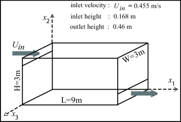
Figure 1: Geometry of the ventilated room.

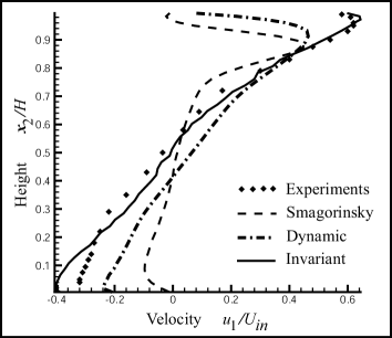
Figure 2: Mean velocity profiles at $x/L=2/3$.

6 Conclusion

In this article, we presented a new class of physically compatible subgrid turbulence models. The main ingredient used is the symmetry group of the Navier–Stokes equations which contains a fundamental information on the properties of the flow. The second principle of thermodynamics was also introduced. From a practical point of view, conformity with this principle ensures stability of the model.

A simple model of the class was tested and encouraging results was obtained. However, the aim of this test was not to present a complete analysis of the model but to check that the symmetry approach can lead to good numerical results. Further studies will be done in future works on the choice of the parameters of the model and on analysis of the numerical results.

The way presented here for deriving symmetry compatible models is a general way. It can be applied to other equations (non-isothermal fluid, …). Other parameters can also be included. For example, dependence of the model on the viscosity $\nu$ can be replaced by dependence on the dissipation rate.

Appendix A Noether’s theorem to Navier–Stokes equations

Noether’s theorem can be applied to evolution equations which can be derived from a Lagrangian, i.e. evolution equations which can be expressed in an Euler–Lagrange form:

$$\cfrac{\partial L(\boldsymbol{r})}{\partial\boldsymbol{r}}\,-\operatorname{Div}\cfrac{\partial L(\boldsymbol{r})}{\partial\dot{\boldsymbol{r}}}\,=0,$$ (30)

where $\boldsymbol{r}$ is the dependent variable, $\boldsymbol{r}=\boldsymbol{r}(\boldsymbol{y})$, $\boldsymbol{y}=(y_{i})_{i}$ the independent variable, $L$ the Lagrangian and $\operatorname{Div}$ the operator:

$$f\mapsto\operatorname{Div}f=\displaystyle{\sum_{i}}\cfrac{\textrm{d}f}{\textrm{d}y_{i}}\,.$$

From the infinitesimal generators of (30), conservation laws are deduced.

Navier–Stokes equations cannot be directly written in the form (30). However, thanks to an approach of Atherton and Homsy [1], see also [10], which consists in extending the Lagrangian notion, it will be shown in this appendix that Noether’s theorem can be applied to Navier–Stokes equations.

We will say that an evolution equation

$$F(\boldsymbol{y},\boldsymbol{r})=0$$ (31)

is derived from a “bi-Lagrangian” if there exists an (non necessarily unique) application

$$L\ :\ (\boldsymbol{r},\boldsymbol{s})\ \mapsto\ L(\boldsymbol{r},\boldsymbol{s})\in\mathbb{R}$$

such that (31) is equivalent to

$$\cfrac{\partial L(\boldsymbol{r},\boldsymbol{s})}{\partial\boldsymbol{s}}\,-\operatorname{Div}\cfrac{\partial L(\boldsymbol{r},\boldsymbol{s})}{\partial\dot{\boldsymbol{s}}}\,=0.$$

$s$ is called the adjoint variable and the equation

$$\cfrac{\partial L(\boldsymbol{r},\boldsymbol{s})}{\partial\boldsymbol{r}}\,-\operatorname{Div}\cfrac{\partial L(\boldsymbol{r},\boldsymbol{s})}{\partial\dot{\boldsymbol{r}}}\,=0$$

is called the adjoint equation of (31). The Noether theorem can then be applied since the evolution equation, associated to his adjoint, can be written in an Euler–Lagrangian form

$$\cfrac{\partial L(\boldsymbol{w})}{\partial\boldsymbol{w}}\,-\operatorname{Div}\cfrac{\partial L(\boldsymbol{w})}{\partial\dot{\boldsymbol{w}}}\,=0,$$

where $\boldsymbol{w}=(\boldsymbol{r},\boldsymbol{s})$.

Navier–Stokes equations are derived from a bi-Lagrangian

$$L((\boldsymbol{u},p),(\boldsymbol{v},q))=\cfrac{1}{2}\left(\cfrac{\partial\boldsymbol{u}}{\partial t}\,\cdot\boldsymbol{v}-\boldsymbol{u}\cdot\cfrac{\partial\boldsymbol{v}}{\partial t}\,\right)+\left(q-\cfrac{1}{2}\ \boldsymbol{u}\cdot\boldsymbol{v}\right)-p\operatorname{div}\boldsymbol{v}+\nu\operatorname{tr}\left({\,{}^{\scriptscriptstyle T}}\nabla\boldsymbol{u}\cdot\nabla\boldsymbol{v}\right).$$

where $\boldsymbol{v}=(v_{i})_{i}$ and $q$ are the adjoint variables. The corresponding adjoint equations are

$$-\cfrac{\partial\boldsymbol{v}}{\partial t}\,+(\boldsymbol{v}\cdot\nabla\boldsymbol{u}{\,{}^{\scriptscriptstyle T}}-\boldsymbol{u}\cdot\nabla\boldsymbol{v})=\nabla q+\nu\Delta\boldsymbol{v},$$

$$\operatorname{div}\boldsymbol{v}=0.$$

Noether’s theorem can then be applied. The infinitesimal generators of the couple of equations (Navier–Stokes equations and their adjoint equations) are:

$$X_{0}=\cfrac{\partial}{\partial t}\,,$$

$$Y_{0}=\zeta(t)\cfrac{\partial}{\partial p}\,,$$

$$X_{ij}=x_{j}\cfrac{\partial}{\partial x_{i}}\,-x_{i}\cfrac{\partial}{\partial x_{j}}\,+u_{j}\cfrac{\partial}{\partial u_{i}}\,-u_{i}\cfrac{\partial}{\partial u_{j}}\,+v_{j}\cfrac{\partial}{\partial v_{i}}\,-v_{i}\cfrac{\partial}{\partial v_{j}}\,,\qquad i=1,2,\quad j>i,$$

$$X_{i}=\alpha_{i}(t)\cfrac{\partial}{\partial x_{i}}\,+\alpha_{i}^{\prime}(t)\cfrac{\partial}{\partial u_{i}}\,-x_{i}\,\alpha_{i}^{\prime\prime}(t)\cfrac{\partial}{\partial p}\,,\qquad i=1,2,3,$$

$$Y_{1}=2t\cfrac{\partial}{\partial t}\,+x_{k}\cfrac{\partial}{\partial x_{k}}\,-u_{k}\cfrac{\partial}{\partial u_{k}}\,-2p\cfrac{\partial}{\partial p}\,-q\cfrac{\partial}{\partial q}\,,$$

$$Y^{\prime}_{0}=\eta(t)\cfrac{\partial}{\partial q}\,,$$

$$X^{\prime}_{ij}=(x_{j}u_{i}-x_{i}u_{j})\cfrac{\partial}{\partial q}\,+x_{j}\cfrac{\partial}{\partial v_{i}}\,-x_{i}\cfrac{\partial}{\partial v_{j}}\,,\qquad i=1,2,\quad j>i,$$

$$X^{\prime}_{i}=\big{(}x_{i}\sigma^{\prime}(t)-u_{i}\sigma(t)\big{)}\cfrac{\partial}{\partial q}\,-\sigma(t)\cfrac{\partial}{\partial v_{i}}\,,\qquad i=1,2,3,$$

$$Y^{\prime}_{1}=v_{k}\cfrac{\partial}{\partial v_{k}}\,+q\cfrac{\partial}{\partial q}\,,$$

where $\zeta$, the $\alpha_{i}$’s, $\eta$ and $\sigma$ are arbitrary scalar functions.

Conservation laws for Navier–Stokes equations can be deduced from these infinitesimal generators. However, that requires non-trivial calculations and is not done in this paper.

In the last section, we will prove that a model which is consistent with the second law of thermodynamics, i.e. such that the total dissipation remains positive, is stable.

Appendix B Stability of thermodynamically consistent models

After an eventual change of variables such that $\boldsymbol{u}$ vanishes along the boundary $\Gamma$ of the domain $\Omega$, the filtered equations can be written in the following form:

$$\cfrac{\partial\overline{\boldsymbol{u}}}{\partial t}\,+\operatorname{div}(\overline{\boldsymbol{u}}\otimes\overline{\boldsymbol{u}})+\cfrac{1}{\rho}\nabla\overline{p}-\operatorname{div}(\overline{\mathsfb{T}}-\mathsfb{T}_{s})=\boldsymbol{F},$$

$$\operatorname{div}\overline{\boldsymbol{u}}=0$$ (32)

associated to the conditions

$$\overline{\boldsymbol{u}}=0\qquad \text{sur}\ \ \Gamma,$$

$$\overline{\boldsymbol{u}}(0,\boldsymbol{x})=\boldsymbol{\gamma}(\boldsymbol{x}) \text{on}\ \ \Omega,$$

$$\displaystyle{\int_{\Omega}\overline{p}(t,\boldsymbol{x})\;\textrm{d}\boldsymbol{x}}=0\qquad \forall\;t\in[0,t_{f}].$$

$\boldsymbol{F}$ is an appropriate function of $t$ and $\boldsymbol{x}$ and $t_{f}$ is the final observation time.

Proposition. Let $(\overline{\boldsymbol{u}},\overline{p})$ be a regular solution of (32) where $\mathsfb{T}_{s}$ is symmetric and verifies the condition:

$$\operatorname{tr}[(\overline{\mathsfb{T}}-\mathsfb{T}_{s})\overline{\mathsfb{S}}]\geq 0.$$

Then:

$$\|\overline{\boldsymbol{u}}(t,\boldsymbol{x})\|_{L^{2}(\Omega)}\leq\|\boldsymbol{\gamma}(\boldsymbol{x})\|_{L^{2}(\Omega)}+\displaystyle{\int_{0}^{t_{f}}\|\boldsymbol{F}(\tau,\boldsymbol{x})\|_{L^{2}(\Omega)}\;\textrm{d}\tau}.$$

This proposition ensures a finite energy when the model conforms to the second law of thermodynamics.

Proof.

Let $({\scriptscriptstyle\bullet},{\scriptscriptstyle\bullet})$ denote the scalar product of $L^{2}(\Omega)$ and $(\overline{\boldsymbol{u}},\overline{p})$ a regular solution of (32). From the first equation of (32) and the boundary condition, we have:

$$\left(\cfrac{\partial\overline{\boldsymbol{u}}}{\partial t}\,,\overline{\boldsymbol{u}}\right)+b(\overline{\boldsymbol{u}},\overline{\boldsymbol{u}},\overline{\boldsymbol{u}})-\cfrac{1}{\rho}\ (p,\operatorname{div}\overline{\boldsymbol{u}})+(\overline{\mathsfb{T}}-\mathsfb{T}_{s},\nabla\overline{\boldsymbol{u}})=(\boldsymbol{F},\overline{\boldsymbol{u}}),$$

where $b$ is defined by the trilinear form

$$b(\boldsymbol{u}^{1},\boldsymbol{u}^{2},\boldsymbol{u}^{3})=\big{(}\operatorname{div}(\boldsymbol{u}^{1}\otimes\boldsymbol{u}^{2}),\boldsymbol{u}^{3}\big{)}.$$

From integrals by parts, the boundary condition and the divergence free condition, it can be shown that $b(\overline{\boldsymbol{u}},\overline{\boldsymbol{u}},\overline{\boldsymbol{u}})=0$ and $(p,\operatorname{div}\overline{\boldsymbol{u}})=0$. Since $(\overline{\mathsfb{T}}-\mathsfb{T}_{s})$ is symmetric, it follows that

$$\left(\cfrac{\partial\overline{\boldsymbol{u}}}{\partial t}\,,\overline{\boldsymbol{u}}\right)+(\overline{\mathsfb{T}}-\mathsfb{T}_{s},\overline{\mathsfb{S}})=(\boldsymbol{F},\overline{\boldsymbol{u}}).$$

Consequently

$$\cfrac{1}{2}\ \cfrac{\textrm{d}}{\textrm{d}t}\,(\overline{\boldsymbol{u}},\overline{\boldsymbol{u}})+(\overline{\mathsfb{T}}-\mathsfb{T}_{s},\overline{\mathsfb{S}})=(\boldsymbol{F},\overline{\boldsymbol{u}}).$$

Now, using the main hypothesis, we have:

$$(\overline{\mathsfb{T}}-\mathsfb{T}_{s},\overline{\mathsfb{S}})=\displaystyle{\int_{\Omega}\operatorname{tr}[(\overline{\mathsfb{T}}-\mathsfb{T}_{s})\overline{\mathsfb{S}}]\;\textrm{d}x}\geq 0$$

and then

$$\cfrac{1}{2}\ \cfrac{\textrm{d}}{\textrm{d}t}\,(\overline{\boldsymbol{u}},\overline{\boldsymbol{u}})\leq(\boldsymbol{F},\overline{\boldsymbol{u}}).$$

Consequently,

$$\|\overline{\boldsymbol{u}}\|_{L^{2}(\Omega)}\cfrac{\textrm{d}}{\textrm{d}t}\,\|\overline{\boldsymbol{u}}\|_{L^{2}(\Omega)}\leq(\boldsymbol{F},\overline{\boldsymbol{u}})\leq\|\boldsymbol{F}\|_{L^{2}(\Omega)}\|\overline{\boldsymbol{u}}\|_{L^{2}(\Omega)}.$$

After simplifying by the $L^{2}$-norm of $\overline{\boldsymbol{u}}$ and integrating over the time, it follows:

$$\|\overline{\boldsymbol{u}}(t,\boldsymbol{x})\|_{L^{2}(\Omega)}\leq\|\boldsymbol{\gamma}(\boldsymbol{x})\|_{L^{2}(\Omega)}+\displaystyle{\int_{0}^{t}\|\boldsymbol{F}(\tau,\boldsymbol{x})\|_{L^{2}(\Omega)}\;\textrm{d}\tau}$$

$$\phantom{\|\overline{\boldsymbol{u}}(t,\boldsymbol{x})\|_{L^{2}(\Omega)}}{}\leq\|\boldsymbol{\gamma}(\boldsymbol{x})\|_{L^{2}(\Omega)}+\displaystyle{\int_{0}^{t_{f}}\|\boldsymbol{F}(\tau,\boldsymbol{x})\|_{L^{2}(\Omega)}\;\textrm{d}\tau}.$$

This ends the proof of the proposition. ∎

References

- [1] Atherton R.W., Homsy G.M., On the existence and formulation of variational principles for nonlinear differential equations, Stud. Appl. Math., 1975, V.54, 31–60.
- [2] Berselli L.C., Grisanti C.R., On the consistency of the rational large eddy simulation model, Comput. Vis. Sci., 2004, V.6, N 2–3, 75–82.
- [3] Bytev V.O., Group-theoretical properties of the Navier–Stokes equations, Numerical Methods of Continuum Mechanics, 1972, V.3, N 3, 13–17 (in Russian).
- [4] Cannone M., Karch G., About the regularized Navier–Stokes equations, J. Math. Fluid Mech., 2005, V.7, 1–28, math.AP/0305097.
- [5] Cantwell B.J., Similarity transformations for the two-dimensional, unsteady, stream-function equation, J. Fluid Mech., 1978, V.85, 257–271.
- [6] Chen Q., Jiang Y., Béhein C., Su M., Particulate dispersion and transportation in buildings with large eddy simulation, Technical Report, Massachusetts Institute of Technology, 2001.
- [7] Danilov Yu.A., Group properties of the Maxwell and Navier–Stokes equations, Preprint, Khurchatov Inst. Nucl. Energy, Acad. Sci. USSR, 1967 (in Russian).
- [8] Fushchych W.I., Popowych R.O., Symmetry reduction and exact solutions of the Navier–Stokes equations, J. Nonlinear Math. Phys., 1994, V.1, 75–113, 156–188, math-ph/0207016.
- [9] Ibragimov N.H., Ünal G., Equivalence transformations of Navier–Stokes equations, İstanbul Tek. Üniv. Bül., 1994, V.47, 203–207.
- [10] Ibragimov N.H., Kolsrud T., Lagrangian approach to evolution equations: symmetries and conservation laws, Nonlinear Dynam., 2004, V.36, 29–40.
- [11] Iliescu T., John V., Layton W., Convergence of finite element approximations of large eddy motion, Numer. Methods Partial Differential Equations, 2002, V.18, 689–710.
- [12] Iliescu T., John V., Layton W.J., Matthies G., Tobiska L., A numerical study of a class of LES models, Int. J. Comput. Fluid Dyn., 2003, V.17, 75–85.
- [13] Kim P., Olver P.J., Geometric integration via multi-space, Regul. Chaotic Dyn., 2004, V.9, N 3, 213–226.
- [14] Lilly D., A proposed modification of the Germano subgrid-scale closure method, Phys. Fluids, 1992, V.4, 633–635.
- [15] Lindgren B., Österlund J., Johansson A., Evaluation of scaling laws derived from Lie group symmetry methods in zero-pressure-gradient turbulent boundary layers, J. Fluid Mech., 2004, V.502, 127–152.
- [16] Méais O., Lesieur M., Spectral large-eddy simulation of isotropic and stably stratified turbulence, J. Fluid Mech., 1992, V.256, 157–194.
- [17] Nielsen P., Restivo A., Whitelaw J., The velocity characteristics of ventilated rooms, J. Fluids Engrg., 1978, V.100, 291–298.
- [18] Oberlack M., Symmetries, invariance and scaling-laws in inhomogeneous turbulent shear flows, Flow, Turbulence and Combustion, 1999, V.62, 111–135.
- [19] Oberlack M., A unified approach for symmetries in plane parallel turbulent shear flows, J. Fluid Mech., 2001, V.427, 299–328.
- [20] Olver P., Geometric foundations of numerical algorithms and symmetry, Appl. Algebra Engrg. Comm. Comput., 2001, V.11, 417–436.
- [21] Razafindralandy D., Contribution à l’étude mathématique et numérique de la simulation des grandes échelles, PHD Thesis, Université de La Rochelle, 2005.
- [22] Sagaut P., Large eddy simulation for incompressible flows. An introduction, Scientific Computation, Springer, 2004.
- [23] Saveliev V., Gorokhovski M., Group-theoretical model of developed turbulence and renormalization of the Navier–Stokes equation, Phys. Rev. E, 2005, V.72, 016302, 6 pages.
- [24] Ünal G., Application of equivalence transformations to inertial subrange of turbulence, Lie Groups Appl., 1994, V.1, 232–240.
- [25] Ünal G., Constitutive equation of turbulence and the Lie symmetries of Navier–Stokes equations, in Modern Group Analysis VII, Editors N.H. Ibragimov, K. Razi Naqvi and E. Straume, Trondheim, Mars Publishers, 1997, 317–323.
- [26] Winckelmans G.S., Wray A., Vasilyev O.V., Jeanmart H., Explicit filtering large-eddy simulation using the tensor-diffusivity model supplemented by a dynamic Smagorinsky term, Phys. Fluids, 2001, V.13, 1385–1403.