Quantitative and Qualitative Study of Gaussian Beam Visualization Techniques

Abstract

We present a comparative overview of existing laser beam profiling methods. We compare the the knife-edge, scanning slit, and pin-hole methods. Data is presented in a comparative fashion. We also elaborate on the use of CCD profiling methods and present appropriate imagery. These methods allow for a quantitative determination of transverse laser beam-profiles using inexpensive and accessible methods. The profiling techniques presented are inexpensive and easily applicable to a variety of experiments.

I Introduction

How large or how ”good” a particular laser beam is, can seem like an infinitely abstract question since a laser beam fades gradually. However, comparing the effects of an expanded laser beam striking a piece of paper with burning a piece of paper with the same focused laser beam brings across the notion that the beam size can make a difference in many physical scenarios. Of course, questions on which methods are appropriate to determine beam quality, divergence and size arise immediately in these types of discussions.

It is a valuable exercise to agree on some type of quantitative definition of a laser beam radius. The standards which the scientific community has agreed upon can then be discussed in a meaningful way.

In general, the irradiance, $I(x,y)$, of an ideal laser beam displays a Gaussian profile as described by Chapple Chapple (1994):

$$I(x,y)=I_{0}\hskip 2.0ptexp\left[-\frac{2((x-x_{0})^{2}+(y-y_{0})^{2})}{r^{2}}\right],$$ (1)

where $I_{0}$ is the peak irradiance at the center of the beam, $x$ and $y$ are the transverse (cross-sectional) cartesian coordinates of any point with respect to the center of the beam located at $(x_{0},y_{0})$, and r is the $1/e^{2}$ beam radius. The definition above assumes a Gaussian distribution for the electric field commonly used in theory. When the electric field expressionPedrotti and Pedrotti (1993) is squared we end up with a factor of 2 in the exponent as shown in Eq. (1). It becomes clear from Eq. (1) that at the radius, r, the irradiance drops to $1/e^{2}$ of its peak value. The Gaussian distribution of the irradiance can also be defined as given by McCally McCally (1984):

$$I(x,y)=I_{0}\hskip 2.0ptexp\left[-\frac{\left((x-x_{0})^{2}+(y-y_{0})^{2}\right)}{R^{2}}\right].$$ (2)

In this case, the beam radius, R, is reached when the irradiance drops to $1/e$ of its maximum value as shown in Fig. 1. Note that the beam radius, r, in Eq. (1) is $\sqrt{2}$ times larger than R.

We will use the definition given by Eq. (1) for the beam radius, r, in this paper.

Figure 1: The Gaussian beam profile of the irradiance, I, is displayed in this two dimensional figure as a function of x. The $1/e^{2}$ beam radius, r, as well as the $1/e$ beam radius, R, are indicated.

We can simply replace the irradiance, I, by the power, P, in equations (1) and  (2), since power and irradiance differ only by a constant factor, i.e., the area. This realization comes in handy during measurements.

The measurement of Gaussian laser beams can be challenging even though the definitions for the size of Gaussian beam are clear.Riza and Mughal (2004); Skinner and Whitcher (1971); Riza and Jorgesen (2004); Khosrofian and Garetz (1983) The challenge in measuring a Gaussian beam profile lies in the nature of the laser light and the properties that are to be determined, i.e., whether the experimentalist is interested in the size of the beam or the beam structure. There are a variety of methods available to measure the properties of Gaussian laser beams. In this paper, we will present a convenient overview of commonly used beam-profiling methods based on the nature of the laser light and the experimental limitations. The data presented here allows for qualitative and quantitative comparison of the various beam-profiling methods.

II Knife-Edge Method

The knife-edge method is a beam profiling method that allows for quick, inexpensive, and accurate determination of the cross-sectional laser beam parameters. The knife-edge method requires a sharp edge (typically a razor blade), a translation stage with a micrometer and a power meter or an energy meter when working with pulses. The knife-edge is translated perpendicular to the direction of propagation of the laser beam. With the knife-edge initially covering the laser beam, the micrometer can be adjusted in appropriate increments. Each data point will show an increase in total power, $P\hskip 0.5pt_{T}$, passing by the knife-edge until the entire beam is detected by the power meter at power $P\hskip 0.5pt_{T0}$ as shown in Fig. 2. The plot shows then the two dimensional Gaussian profile integrated over the displacement of the razor blade, $x$, which is the Error function, $erf(x)$, describing the total power, $P\hskip 0.5pt_{T}$, bypassing the knife edge:

$$P\hskip 0.5pt_{T}(x)=P_{0}r\sqrt{\frac{\pi}{8}}\hskip 2.0pterf\left[\frac{\sqrt{2}\hskip 1.0ptx}{r}\right].$$ (3)

Figure 2: (a) A Coherent Verdi laser was used for the collection of this sample data. The total power, $P_{T}$, passing by the knife-edge is shown as a function of knife-edge displacement. (b) The derivative of the knife-edge data is found by using Eq. (4). The $1/e^{2}$ radius, r, is $1270\mu m\pm 20\mu m$.

There are several ways to evaluate the $1/e^{2}$ radius using this type of data:

1. Fitting the Error function and evaluating fitted parameters in accordance with Eq. (3). This is, however, a more involved procedure based on the mathematical nature of the error function, we do not recommend a fit to the error function for practical reasons and for quick results. We reserve the discussion of this method for another paper.

2. Taking the derivative of the data using an algorithm that allows for smoothing of the derivative is practical. In this case, the derivative at any data point was taken by averaging the derivative of two adjacent data points:

   $$\frac{dP_{T}}{dx}=\frac{1}{2}\left(\frac{y_{i+1}-y_{i}}{x_{i+1}-x_{i}}+\frac{y_{i}-y_{i-1}}{x_{i}-x_{i-1}}\right),$$ (4)

   gives the power at a particular point $x$ in the beam as shown in Fig 2b. This type of derivative may be taken quickly by using spreadsheets. The students then have two options of finding the $1/e^{2}$ radius, r:

   1. One can simply estimate by dividing the maximum value in the derivative plot by $e^{2}$ and finding the corresponding r value by linear extrapolation between points.

   2. Alternatively, a Gaussian can be fit to the data in Fig 2b using one of the widely available data analysis programs. This will also allow for a quick assessment of the experimental error associated with this fit. We used Origin 7.5 in this case. It is then instructive to compare these results with the method described in 2a.

A few data points are sufficient to determine the size of a Gaussian laser beam to very high accuracy, limited by the resolution of the translation stage and the stability of the laser. Using a relatively inexpensive mechanical micrometer, the resolution can be $2\mu m$ or betterPlass et al. (1997). Diffraction does not have a significant impact since the light does not spread significantly after passing the knife-edge. The knife-edge can therefore fit in easily at any point an optical set-up while the detector can be conveniently placed after the knife-edge, depending on the spatial configuration of the setup.

A drawback of the knife-edge method is the lack of resolved features in the resulting beam-profile. Since we are measuring the integral of the Gaussian beam, features such as hot-spots disappear. Taking too many data points can be a disadvantage since any noise will be amplified by taking the derivative. Keeping the number of data points to a minimum will ensure a smoother fit. Methods allowing for a more detailed examination of the beam-profile are discussed in the following sections.

III Slit Method

Using a slit to obtain a beam profile can be achieved by simply replacing the Knife-Edge in section II by a narrow slit. We used a $7\mu m$ slit to confirm the data we obtained with the knife-edge. Since we obtain the same error for the $1/e^{2}$ radius, r, for both methods, we see that in this case most of the error originates from instabilities in the laser beam independently of the method chosen, i.e., more accurate results can only be obtained with a more stable laser.

The slit method assumes that the slit is infinitely narrow so that we can map the power transmitted through the slit at any point of the profile. We can therefore use the slit as long as it is much narrower than the beam. The data can then be plotted directly as shown in Fig. 3.

Figure 3: The same Coherent Verdi laser used in the knife-edge measurement was used for the collection of this sample data. The power, $P$, passing through a $7\mu m$ slit is shown as a function of slit displacement. The $1/e^{2}$ radius, r, is found to agree with the results reported in section II ($1270\mu m\pm 20\mu m$).

Traditionally slits have been used as a profiling method when the slit width is much smaller than the beam itself as it is the case in our example. Nevertheless, a slit may also be used when the slit width is about the same size as the laser beam when measuring the beam waist, $w_{0}$, of a focused beam as ChappleChapple (1994) has shown:

$$w_{0}^{2}=w_{0s}^{2}-\frac{s^{2}}{3},$$ (5)

where $w_{0s}^{2}$ is the uncorrected size of the beam waist, and $s$ is the width of the slit.

Even though slits are most appropriate for large beams, care must be taken that the results are not distorted by the beam exceeding the longitudinal dimension of the slit. Diffraction is not an issue as long as the detector is positioned close enough to the slit to collect the light after passing through the slit before it spreads beyond the dimensions of the detector. A lens can be used right after the slit to collect the diffracted light if the detector cannot be placed immediately after the slit.

Finally, the slit method may be impractical when measuring low power beams since only a very narrow slice of the laser beam passes through the slit. This power drop becomes evident when comparing Figs. 2 and 3.

As with the Knife-Edge method, the Slit method does not reveal beam profile features like hot spots. However, these methods are most practical for determining the size of a Gaussian laser beam.

IV Pinhole Method

The pinhole method allows the user to scan across a laser beam and record the irradiance at every point. This technique allows for the collection of a highly resolved beam profile. Hot spots and other beam features can then be detected. Intensity distributions across a laser beam become critical for experiments involving optical non-linearities.

Figure 4: The same Coherent Verdi laser beam was probed for the collection of this sample data. Difficulty in locating beam center and the exact location of the pinhole inside the BeamProfiler by Photon Inc., contributed to the systematic error which resulted in a measured beam width of $1110\mu m\pm 10\mu m$ deviating from the results of sections II and  III.

The beam profile in Fig. 4 was obtained using an computer controlled pinhole by Photon Inc. It is impractical to mount a pinhole on a translation station and take the data manually as we did when we used the knife-edge or slit. It is more advantageous to use the pinhole in an automated system that allows for quicker data collection. In our case, the pinhole and sensor are contained in one unit so that the exact position of the pinhole and sensor could not be located easily. Also, there is no insight into the mechanism of determining the beam center for the horizontal sweep of the pinhole resulting in another possible source of systematic error. These two systematic errors account for a beam width of $1110\mu m\pm 10\mu m$ deviating from the results in sections II and  III by $160\mu m$.

The light passing through the pinhole is significantly reduced in intensity compared to the slit and therefore even harder to detect and more prone to poor signal to noise ratio issues. It should be noted that it can be difficult to sweep exactly across the center of the laser beam. The beam can thus appear smaller than it really is.

V CCD Cameras

Quick qualitative analysis of transverse laser beam profiles can be achieved through the use of CCD cameras as shown in Fig. 5. Visual inspection of this beam profile reveals not only an almost elliptical shape but also other irregularities in the profile.

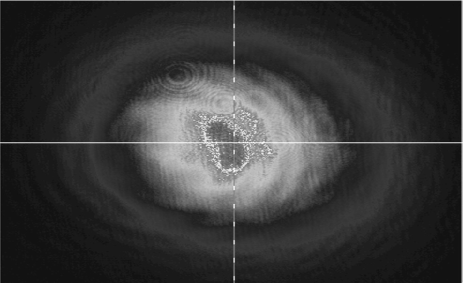
Figure 5: CCD image of CW Verdi laser beam. The image reveals a somewhat elliptical shape that shows a combination of modes. Artifacts from due to interference are visible.

There are many different types of CCD cameras available. The resolution of a CCD camera is governed by pixel-size and number of pixels. An adjustable dark current can prevent the CCD camera from saturating without the use of attenuators. An inexpensive digital camera can also be used to capture a beam profile as long as the beam is carefully attenuated to prevent saturation or damage to the camera. It should be noted that attenuation tends to distort the beam profile and beam size. High-intensity or pulsed lasers may introduce non-linearities in experimental camera optics leading to a distorted beam profile. Interference effects originating from dust and the use of a neutral density filter are visible in Fig. 5 and should not be confused with beam features.

VI Creating a Beam Map

The knife-edge method can even be used to determine beam overlap and relative beam propagation when using several beams. Also, beam divergence can be determined by measuring the beam radius at various points along the beam path. The type of beam propagation data shown in Fig. 6 is useful in many research projects or may simply be used to demonstrate Gaussian beam propagation in an undergraduate laboratory.Pedrotti and Pedrotti (1993)

Figure 6: A map of two pulsed laser beams is created to verify beam overlap around experimental focal points. The laser used is a Continuum Leopard picosecond system. (a) A side view of the beam divergence is presented. (b) The center positions of the beams are mapped in a top view to evaluate beam overlap. The laser beam shown in the solid line needs to be adjusted horizontally to ensure overlap at $z=0mm$. The error is around $1\%$ for each data point and too small to show on this scale.

VII Conclusion

We have demonstrated the reliability of the knife-edge and slit beam-profiling methods in determining the size of a Gaussian laser beam by presenting the identical results of $1270\mu m\pm 20\mu m$ for the beam radius for both methods whereas the pinhole method shows deviations as presented above. Furthermore, we have presented two beam profiling methods, the CCD array and the pinhole method, in evaluating beam quality. There are many sophisticated beam profiling instruments that are commercially available. Nevertheless, beam profiles can be obtained effectively with modest resources. Most of the commercially available beam profilers are based on the principles outlined in this paper. Under certain circumstances, it can certainly be convenient and a time saver to purchase a beam profiling system.