Divergent Time Scale in Axelrod Model Dynamics

Abstract

We study the evolution of the Axelrod model for cultural diversity. We consider a simple version of the model in which each individual is characterized by two features, each of which can assume $q$ possibilities. Within a mean-field description, we find a transition at a critical value $q_{c}$ between an active state of diversity and a frozen state. For $q$ just below $q_{c}$, the density of active links between interaction partners is non-monotonic in time and the asymptotic approach to the steady state is controlled by a time scale that diverges as $(q-q_{c})^{-1/2}$.

A basic feature of many societies is the tendency to form distinct cultural domains even though individuals may rationally try to reach agreement with acquaintances. The Axelrod model provides a simple yet rich description for this dichotomy by incorporating societal diversity and the tendency toward consensus by local interactions A . In this model, each individual carries a set of $F$ characteristic features that can assume $q$ distinct values; for example, one’s preferences for sports, for music, for food, etc. In an elemental update step, a pair of interacting agents $i$ and $j$ is selected. If the agents do not agree on any feature, then there is no interaction. However, if the agents agree on at least one feature, then another random feature is selected and one of the agents changes its preference for this feature to agree with that of its interaction partner. A similar philosophy of allowing interactions only between sufficiently compatible individuals underlies related systems, such as bounded confidence compromise and constrained voter-like models VR .

Depending on the two parameters $F$ and $q$, a phase transition occurs between cultural homogeneity, where all agents are in the same state, and diversity A ; CMV ; VVC ; KETM . The latter state could either be frozen, where no pair of interacting agents shares any common feature, or it could be continuously evolving if pairs with shared features persist. The rich dynamics of the model does not fall within the classical paradigms of coarsening in an interacting spin system spins or diffusive approach to consensus in the voter model voter . In this Letter, we solve mean-field master equations for Axelrod model dynamics and show that the approach to the steady state is non-monotonic and extremely slow, with a characteristic time scale that diverges as $q\to q_{c}$ (Figs. 1 & 2).

The emergence of an anomalously long time scale is unexpected because the underlying master equations have rates that are of the order of one. Another important example of wide time-scale separation occurs in HIV hiv . After an individual contracts the disease, there is a normal immune response over a time scale of months, followed by a latency period that can last beyond 10 years, during which an individual’s T-cell level slowly decreases with time. Finally, after the T-cell level falls below a threshold value, there is a final fatal phase that lasts 2–3 years. Our results for the Axelrod model may provide a hint toward understanding how widely separated time scales arise in these types of complex dynamical systems.

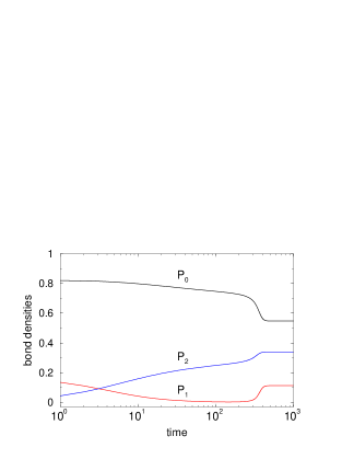
Figure 1: Master-equation time dependence of bond densities $P_{0}$, $P_{1}$, and $P_{2}$ for $q=q_{c}-4^{-1}$. Each agent has 4 neighbors.

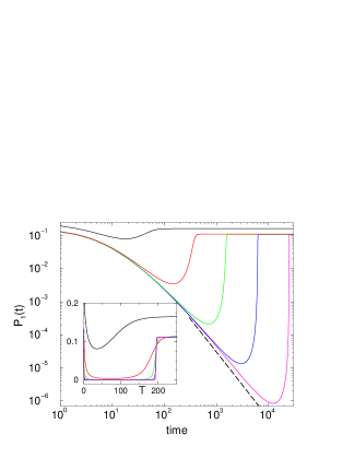
Figure 2: Master-equation result for $P_{1}(t)$ for $q=q_{c}-4^{-k}$, with $k=-1,1,3,5$, and $7$ (progressively lower minima). Each agent has 4 neighbors. The dashed line has slope $-2$ (see text). Inset: Same data on a linear scale with $T=t(q-q_{c})^{1/2}$.

Following Refs. CMV ; VVC , we describe the Axelrod model in a minimalist way by the density $P_{m}$ of bonds of type $m$. These are bonds between interaction partners in which there are $m$ common features. This description is convenient for monitoring the activity level in the system and has the advantage of being analytically tractable. We consider a mean-field system in which each agent can interact with a fixed number of randomly-selected agents. Agents can thus be viewed as existing on the nodes of a degree-regular random graph. Such a topology is an appropriate setting for cultural interaction, where both geographically nearby and distant individuals may interact with equal facility. We verified that simulations of the Axelrod model on degree-regular random graphs qualitatively agree with our analytical predictions, and this agreement becomes progressively more accurate as the number of neighbors increases (Fig. 3). Thus the master equation approach describes the Axelrod model when random connections between agents exist.

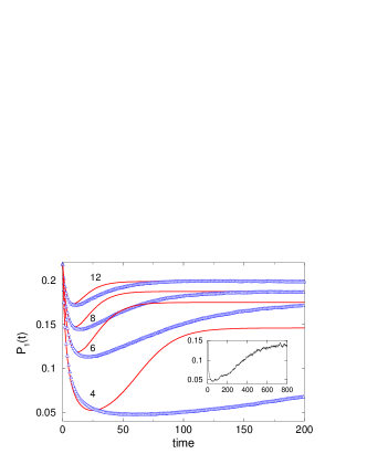
Figure 3: Active bond density from the master equations (curves) and from simulations of $10^{2}$ realizations ($\triangle$) on a degree-regular random graph with $10^{4}$ nodes for various coordination numbers, and $q=8$ states per feature. Inset: One realization with coordination number 4.

If interaction partners share no common features ($m=0$) or if all features are common ($m=F$), then no interaction occurs across the intervening bond. Otherwise, two agents that are connected by an active bond of type $m$ (with $0<m<F$) interact with probability $m/F$, after which the bond necessarily becomes type $m+1$. In addition, when an agent changes a preference, the index of all bonds attached to this agent may either increase or decrease (Fig. 4). The competition between these direct and indirect interaction channels underlies the rich dynamics of the Axelrod model.

Figure 4: Illustration of the state-changing bond updates when agent $j$ changes state from $a_{1}b_{2}\to a_{1}b_{1}$. The values at the right give the relative rates of each type of event.

Because we obtain qualitatively similar behavior for the density of active links, $P_{a}\equiv\sum_{k=1}^{F-1}P_{k}$, for all $F\geq 2$, we focus on the simplest non-trivial case of $F=2$. For this example, there are three types of bonds: bonds of type $0$ (no shared features) and type $2$ (all features shared) are inert, while bonds of type $1$ are active. As $q\to q_{c}$ from below, $P_{1}$ is non-monotonic, with an increasingly deep minimum (Fig. 2), while for $q>q_{c}$, $P_{1}$ decays to zero exponentially with time. There is a discontinuous transition at $q_{c}$ from a stationary phase where the steady-state density of active links $P_{a}^{s}$ is greater than zero to a frozen phase where $P_{1}^{s}=0$.

When fluctuations are neglected, the evolution of the bond densities $P_{m}$ when a single agent changes its state is described by the master equations:

$$\frac{dP_{0}}{dt} \!=\! \frac{\eta}{\eta\!+\!1}P_{1}\left[-\lambda P_{0}+\frac{1}{2}P_{1}\right]\,,$$ (1)

$$\frac{dP_{1}}{dt} \!=\! \!-\frac{P_{1}}{\eta\!+\!1}+\frac{\eta}{\eta\!+\!1}P_{1}\!\left[\lambda P_{0}-\frac{1\!+\!\lambda}{2}P_{1}+P_{2}\right],$$ (2)

$$\frac{dP_{2}}{dt} \!=\! \frac{P_{1}}{\eta\!+\!1}+\frac{\eta}{\eta\!+\!1}P_{1}\left[\frac{\lambda}{2}P_{1}-P_{2}\right]\,,$$ (3)

where $\eta+1$ is the network coordination number. The first term on the right-hand sides of Eqs. (2) and (3) account for the direct interaction between agents $i$ and $j$ that changes a bond of type $1$ to type $2$. For example, in the equation for $\frac{dP_{1}}{dt}$, a type-1 bond and the shared feature across this bond is chosen with probability $P_{1}/2$ in an update event. This update decrements the number of type-1 bonds by one in a time $dt=\frac{1}{N}$, where $N$ is the total number of sites in the system. Assembling these factors gives the term $-\frac{P_{1}}{\eta+1}$ in Eq. (2).

The remaining terms in the master equations represent indirect interactions. For example, if agent $j$ changes from $(a_{1},b_{2})$ to $(a_{1},b_{1})$ then the bond to agent $k$ in state $(a_{1},b_{1})$ changes from type 1 to type 2 (Fig. 4). The probability for this event is proportional to $P_{1}\lambda/2$: $P_{1}$ accounts for the probability that the indirect bond is of type 1, the factor 1/2 accounts for the fact that only the first feature of agents $j$ and $k$ can be shared, while $\lambda$ is the conditional probability that $i$ and $k$ share one feature that is simultaneously not shared with $j$. If the distribution of preferences is uniform, then $\lambda=(q-1)^{-1}$. As the system evolves $\lambda$ generally depends on the densities $P_{m}$. Here we make an assumption of a mean-field spirit that $\lambda$ stays constant during the dynamics VVC ; this makes the master equations tractable. Our simulations for random graphs with large coordination number match the master equation predictions and give $\lambda$ nearly constant and close to $(q-1)^{-1}$ (Fig. 3), thus justifying the assumption.

Let us first determine the stationary solutions of the master equations. A trivial steady state is $P_{1}^{s}=0$, corresponding to a static society. A more interesting stationary solution is $P_{1}^{s}>0$, corresponding to continuous evolution; as we shall see, this dynamic state arises when $q<q_{c}$. Setting $\frac{dP_{i}}{dt}=0$ in the master equations and solving, we obtain:

$$P_{0}^{s} = \frac{(\eta-1)}{\eta(1+\lambda)^{2}}\,,\quad P_{1}^{s}=\frac{2\lambda(\eta-1)}{\eta(1+\lambda)^{2}}\,,$$

$$P_{2}^{s} = \frac{(1+\lambda)^{2}+\lambda^{2}(\eta-1)}{\eta(1+\lambda)^{2}}.$$ (4)

Since $\lambda=\lambda(q)$ is the only parameter in the master equations, the two stationary solutions suggest that there is a transition at a critical value $q_{c}$ such that both solutions apply, but on different sides of the transition. To locate the transition, it proves useful to relate $P_{1}$ and $P_{2}$ directly. Thus we divide Eq. (2) by Eq. (3) and eliminate $P_{0}$ via $P_{0}=1-P_{1}-P_{2}$ and obtain, after some algebra:

$$\frac{dP_{1}}{dP_{2}}=\frac{-1+\eta\lambda-\frac{1}{2}\eta(1+3\lambda)P_{1}+\eta(1-\lambda)P_{2}}{1+\frac{1}{2}\eta\lambda P_{1}-\eta P_{2}}\,.$$ (5)

The solution to Eq. (5) has the form

$$P_{1}=\alpha+\beta P_{2}-\sqrt{\gamma+\delta P_{2}}\,,$$ (6)

where we determine the coefficients $\alpha$, $\beta$, $\gamma$ and $\delta$ by matching terms of the same order in Eq. (5) and in $\frac{dP_{1}}{dP_{2}}$ from Eq. (6). The procedure gives the solution except for one constant that is specified by the initial conditions. For the initial condition where features for each agent are chosen uniformly from the integers $[0,q-1]$, the distribution of initial bond densities is binomial, $P_{m}(t=0)=\frac{2!}{m!(2-m)!}(1/q)^{m}(1-1/q)^{2-m}$. Matching this initial condition to the solution of Eq. (6) gives:

$$P_{1}(P_{2}) = \frac{2\lambda}{1+\lambda}+\frac{2}{\eta}-2P_{2}$$ (7)

$$~{}~{}~{}~{}-\frac{2}{\eta}\frac{\sqrt{\eta\lambda^{2}+(1+\lambda)^{2}(1-\eta P_{2})}}{(1+\lambda)}\,.$$

As a function of $P_{2}$, $P_{1}$ has a minimum $P_{1}^{\rm min}(q)$ that monotonically decreases as $q$ increases and becomes negative for $q$ larger than a critical value $q_{c}$ (Fig. 5). The phase transition between the active and the frozen state corresponds to the value of $q$ where $P_{1}$ first reaches zero. To find $q_{c}$, we calculate $P_{1}^{\rm min}$ as a function of $\lambda(q)$ from Eq. (7) and then find the value of $q$ at which $P_{1}^{\rm min}$ becomes zero. This leads to

$$P_{1}^{\rm min}=\frac{4\eta\lambda-(1+\lambda)^{2}}{2\eta(1+\lambda)^{2}}\equiv\frac{S(\lambda,\eta)}{2\eta(1+\lambda)^{2}}\,,$$

from which the critical point is given by

$$q_{c} = 2\eta+2\sqrt{\eta(\eta-1)}\,,$$

while $P_{1}^{\rm min}\propto S\propto(q_{c}-q)$ for $q<q_{c}$.

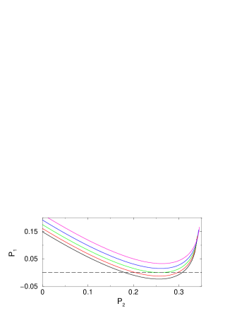
Figure 5: $P_{1}$ vs $P_{2}$ from Eq. (7) for $\eta=3$ and $q=q_{c}-2$, $q_{c}-1$, $q_{c}$, $q_{c}+1$ and $q_{c}+2$ (top to bottom).

We now determine the steady-state bond densities in the frozen state. From Eq. (7), we compute the stationary value $P_{2}^{s}$ at the point where $P_{1}$ first reaches zero. The smallest root of this equation then gives

$$P_{2}^{s}=\frac{1+\lambda+2\eta\lambda-\sqrt{(1+\lambda)^{2}-4\eta\lambda}}{2\eta(1+\lambda)}\,,$$

while $P_{0}^{s}=1-P_{2}^{s}$.

The most interesting behavior is the time dependence of the density of active bonds, $P_{1}(t)$. We solve for $P_{1}(t)$ by first inverting Eq. (7) to express $P_{2}$ in terms of $P_{1}$

$$P_{2}(P_{1})=\frac{1+\lambda(1+2\eta)}{2\eta(1+\lambda)}-\frac{P_{1}}{2}-\frac{\sqrt{2\eta(1+\lambda)^{2}P_{1}-S}}{2\eta(1+\lambda)}\,,$$

and then writing $P_{0}=1-P_{1}-P_{2}(P_{1})$ also in terms of $P_{1}$, and finally substituting these results into the master equation (2) for $P_{1}$. After some algebra, we obtain

$$\frac{dP_{1}}{d\tau} = SP_{1}-(1-\lambda)\sqrt{2\eta(1+\lambda)^{2}P_{1}-S\,}\,P_{1}$$ (8)

$$~{}~{}~{}~{}~{}~{}-2\eta(1+\lambda)^{2}P_{1}^{2},$$

where we use the rescaled time variable $\tau=\frac{t}{2(\eta+1)(1+\lambda)}$. This master equation can be simplified by substituting the quantity $\Delta\equiv 2\eta(1+\lambda)^{2}P_{1}-S$, which measures the deviation of $P_{1}$ from its minimum value, in Eq. (8). We obtain

$$\frac{d\Delta}{d\tau}=-\sqrt{\Delta}(S+\Delta)(1-\lambda+\sqrt{\Delta})\,.$$ (9)

Performing this integral by partial fraction expansion gives

$$\tau=\frac{1}{4\lambda(\eta-1)}\Biggl{[}\ln\left(\frac{S+\Delta}{\eta\lambda(1-\lambda)^{2}}\right)-2\ln\left(1\pm\frac{\sqrt{\Delta}}{1-\lambda}\right)$$

$$+\frac{1-\lambda}{\sqrt{-S}}\ln\left(\frac{(\sqrt{-S}-1-\lambda)(\sqrt{-S}\pm\sqrt{\Delta})}{(\sqrt{-S}+1+\lambda)(\sqrt{-S}\mp\sqrt{\Delta})}\right)\Biggr{]}\,.$$

For $q>q_{c}$, only the upper sign is needed. For $q<q_{c}$, the upper sign applies for $t<t^{\rm min}$ and the lower sign applies for $t>t^{\rm min}$; here $t^{\rm min}$ is the time at which $P_{1}(t)$ reaches its minimum value. Substituting back $t$ and $P_{1}$ in Eq. (Divergent Time Scale in Axelrod Model Dynamics) gives the formal exact solution of Eq. (8).

For $q<q_{c}$, we determine $P_{1}(t)$ near its minimum by taking the $\Delta\to 0$ limit of Eq. (9). This gives

$$\frac{d\Delta}{dt}\approx-aS\sqrt{\Delta}\,,$$ (11)

with $a=\frac{(1-\lambda)}{2(\eta+1)(1+\lambda)}>0$. For $S>0$, the solution to the lowest-order approximation shows that $P_{1}$ has a quadratic form around its minimum:

$$P_{1}(t)-P_{1}^{\rm min}\propto\Delta\approx\frac{a^{2}S^{2}}{8\eta(1+\lambda)^{2}}(t-t_{\rm min})^{2}\,.$$ (12)

When $q\to q_{c}$, the factor $S$ may be neglected as long as $\Delta>S$, and this leads to $\Delta$ decaying as $t^{-2}$ before the minimum in $P_{1}$ is reached (dashed line in Fig. 2).

The peculiar behavior of $P_{1}$ as a function of time for $q$ below but close to the critical value $q_{c}$ is shown in Fig. 2. The density of active bonds quickly decreases with time and this decrease extends over a wide range when $q$ is close to $q_{c}$. Thus on a linear scale, $P_{1}$ remains close to zero for a substantial time. After a minimum value at $t_{\rm min}$ is reached, $P_{1}$ then increases and ultimately reaches a non-zero asymptotic value for $q<q_{c}$. The quasi-stationary regime where $P_{1}$ remains small is defined by: (i) a time scale of the order of one that characterizes the initial decay of $P_{1}(t)$, and (ii) a much longer time scale $t_{\rm asymp}$ where $P_{1}$ rapidly increases and then saturates at its steady-state value.

We can give a partial explanation for the time dependence of $P_{1}$. For $q>q_{c}$, there are initially small enclaves of interacting agents in a frozen discordant background. Once these enclaves reach local consensus, they are incompatible with the background and the system freezes. For $q\lesssim q_{c}$ (less diversity), sufficient active interfaces are present to slowly and partially coarsen the system into tortuous domains whose occupants are either compatible (that is, interacting) or identical. Within a domain of interacting agents, the active interface can ultimately migrate to the domain boundary and facilitate merging with other domains; this corresponds to the sharp drop in $P_{0}$ seen in Fig. 1 applet . While this picture is presented in the context of a lattice system, it remarkably still seems to apply for degree-regular random graphs and in a mean-field description.

Both $t_{\rm min}$ as well as the end time of the quasi-stationary period $t_{\rm asymp}$ increase continuously and diverge as $q$ approaches $q_{c}$ from below. To find these divergences, we expand $t_{\rm min}$ and $t_{\rm asymp}$ in powers of $S$. From Eq. (Divergent Time Scale in Axelrod Model Dynamics), the first two terms in the expansion of $t_{\rm min}$, as $S\to 0$, are

$$t_{\rm min}=t(P_{1}^{\rm min})\approx A\ln S+\frac{B}{\sqrt{S}}\sim\frac{B}{\sqrt{S}}\,,$$

where $A,B$ are constants. As a result, $t_{\rm min}\sim(q_{c}-q)^{-1/2}$ as $q\to q_{c}$. Similarly, we estimate $t_{\rm asymp}$ as the time at which $P_{1}$ reaches one-half of its steady-state value. Using Eqs. (Divergent Time Scale in Axelrod Model Dynamics) and (Divergent Time Scale in Axelrod Model Dynamics), we find

$$t_{\rm asymp}=t(P_{1}^{s}/2)\sim\frac{1}{\sqrt{S}}\;\;\mbox{as}\;\;S\to 0\,,$$

so that $t_{\rm asymp}\sim(q_{c}-q)^{-1/2}$ as $q\to q_{c}$.

For $q>q_{c}$, the system evolves to a frozen state with $P_{1}\to 0$. To lowest order Eq. (8) becomes $\frac{dP_{1}}{dt}=-\frac{P_{1}}{\mathcal{T}}$, with $\mathcal{T}=\frac{2(\eta+1)(1+\lambda)}{-S+(1-\lambda)\sqrt{-S}}$. Here $\mathcal{T}>0$ since $S<0$ for $q>q_{c}$. Consequently $P_{1}$ decays exponentially in time as $t\to\infty$. As $q$ approaches $q_{c}$, $S$ asymptotically vanishes as $(q_{c}-q)$ and the leading behavior is $\mathcal{T}\sim(q-q_{c})^{-1/2}\,$. Thus again there is an extremely slow approach to the asymptotic state as $q$ approaches $q_{c}$.

In summary, the density of active links is non-monotonic in time and is governed by an anomalously long time scale in the 2-feature and q preferences per feature Axelrod model. For $q<q_{c}$, an active steady-state state is reached in a time that diverges as $(q_{c}-q)^{-1/2}$ when $q\to q_{c}$ from below. For $q>q_{c}$, the final state is static and the time scale to reach this state also diverges as $(q_{c}-q)^{-1/2}$ as $q\to q_{c}$ from above.

We gratefully acknowledge financial support from the US National Science Foundation grant DMR0535503.

References

- (1) R. Axelrod, J. Conflict Res. 41, 203 (1997); R. Axtell, R. Axelrod, J. Epstein, and M. D. Cohen, Comput. Math. Organiz. Theory 1, 123 (1996).
- (2) G. Weisbuch, G. Deffuant, F. Amblard, and J. P. Nadal, Complexity 7, 55 (2002); E. Ben-Naim, P. L. Krapivsky, and S. Redner, Physica D 183, 190 (2003).
- (3) F. Vazquez, S. Redner J. Phys. A 37, 8479 (2004).
- (4) C. Castellano, M. Marsili, and A. Vespignani, Phys. Rev. Lett. 85, 3536 (2000).
- (5) D. Vilone, A. Vespignani, and C. Castellano, Eur. Phys. J. B 30, 399 (2002).
- (6) K. Klemm, V. M. Eguiluz, R. Toral, and M. San Miguel, Phys. Rev. E 67, 026120 (2003); K. Klemm, V. M. Eguiluz, R. Toral, and M. San Miguel, cond-mat/0205188; cond-mat/0210173; physics/0507201
- (7) R. J. Glauber, J. Math. Phys. 4, 294 (1963); J. D. Gunton, M. San Miguel, and P. S. Sahni in: Phase Transitions and Critical Phenomena, Vol. 8, eds. C. Domb and J. L. Lebowitz (Academic, NY 1983); A. J. Bray, Adv. Phys. 43, 357 (1994).
- (8) T. M. Liggett, Interacting Particle Systems (Springer-Verlag, New York, 1985); P. L. Krapivsky, Phys. Rev. A 45, 1067 (1992).
- (9) See e.g., A. S. Perelson, P. W. Nelson, SIAM Review 41, 3 (1999)
- (10) For a java applet to visualize these phenomena, see http://www.imedea.uib.es/physdept/researchtopics/ socio/culture.html.