Finding community structure in networks using the eigenvectors of matrices

Abstract

We consider the problem of detecting communities or modules in networks, groups of vertices with a higher-than-average density of edges connecting them. Previous work indicates that a robust approach to this problem is the maximization of the benefit function known as “modularity” over possible divisions of a network. Here we show that this maximization process can be written in terms of the eigenspectrum of a matrix we call the modularity matrix, which plays a role in community detection similar to that played by the graph Laplacian in graph partitioning calculations. This result leads us to a number of possible algorithms for detecting community structure, as well as several other results, including a spectral measure of bipartite structure in networks and a new centrality measure that identifies those vertices that occupy central positions within the communities to which they belong. The algorithms and measures proposed are illustrated with applications to a variety of real-world complex networks.

I Introduction

Networks have attracted considerable recent attention in physics and other fields as a foundation for the mathematical representation of a variety of complex systems, including biological and social systems, the Internet, the worldwide web, and many others [1, 2, 3, 4]. A common feature of many networks is “community structure,” the tendency for vertices to divide into groups, with dense connections within groups and only sparser connections between them [5, 6]. Social networks [5], biochemical networks [7, 8, 9], and information networks such as the web [10], have all been shown to possess strong community structure, a finding that has substantial practical implications for our understanding of the systems these networks represent. Communities are of interest because they often correspond to functional units such as cycles or pathways in metabolic networks [8, 9, 11] or collections of pages on a single topic on the web [10], but their influence reaches further than this. A number of recent results suggest that networks can have properties at the community level that are quite different from their properties at the level of the entire network, so that analyses that focus on whole networks and ignore community structure may miss many interesting features.

For instance, in some social networks one finds individuals with different mean numbers of contacts in different groups; the individuals in one group might be gregarious, having many contacts with others, while the individuals in another group might be more reticent. An example of this behavior is seen in networks of sexual contacts, where separate communities of high- and low-activity individuals have been observed [12, 13]. If one were to characterize such a network by quoting only a single figure for the average number of contacts an individual has, one would be missing features of the network directly relevant to questions of scientific interest such as epidemiological dynamics [14].

It has also been shown that vertices’ positions within communities can affect the role or function they assume. In social networks, for example, it has long been accepted that individuals who lie on the boundaries of communities, bridging gaps between otherwise unconnected people, enjoy an unusual level of influence as the gatekeepers of information flow between groups [15, 16, 17]. A surprisingly similar result is found in metabolic networks, where metabolites that straddle the boundaries between modules show particular persistence across species [8]. This finding might indicate that modules in metabolic networks possess some degree of functional independence within the cell, allowing vertices central to a module to change or disappear with relatively little effect on the rest of the network, while vertices on the borders of modules are less able to change without affecting other aspects of the cellular machinery.

One can also consider the communities in a network themselves to form a higher level meta-network, a coarse-grained representation of the full network. Such coarse-grained representations have been used in the past as tools for visualization and analysis [18] but more recently have also been investigated as topologically interesting entities in their own right. In particular, networks of modules appear to have degree distributions with interesting similarities to but also some differences from the degree distributions of other networks [9], and may also display so-called preferential attachment in their formation [19], indicating the possibility of distinct dynamical processes taking place at the level of the modules.

For all of these reasons and others besides there has been a concerted effort in recent years within the physics community and elsewhere to develop mathematical tools and computer algorithms to detect and quantify community structure in networks. A huge variety of community detection techniques have been developed, based variously on centrality measures, flow models, random walks, resistor networks, optimization, and many other approaches [5, 20, 21, 22, 23, 18, 24, 25, 26, 27, 28, 29, 9, 8, 30, 31, 32, 33, 34, 35]. For reviews see Refs. [6, 36].

In this paper we focus on one approach to community detection that has proven particularly effective, the optimization of the benefit function known as “modularity” over the possible divisions of a network. Methods based on this approach have been found to produce excellent results in standardized tests [36, 37]. Unfortunately, exhaustive optimization of the modularity demands an impractically large computational effort, but good results have been obtained with various approximate optimization techniques, including greedy algorithms [24, 38], simulated annealing [39, 34], and extremal optimization [40]. In this paper we describe a different approach, in which we rewrite the modularity function in matrix terms, which allows us to express the optimization task as a spectral problem in linear algebra. This approach leads to a family of fast new computer algorithms for community detection that produce results competitive with the best previous methods. Perhaps more importantly, our work also leads to a number of useful insights about network structure via the close relations we will demonstrate between communities and matrix spectra.

Our work is by no means the first to find connections between divisions of networks and matrix spectra. There is a large literature within computer science on so-called spectral partitioning, in which network properties are linked to the spectrum of the graph Laplacian matrix [41, 42, 43]. This method is different from the one introduced here and is not in general well suited to the problem of community structure detection. The reasons for this, however, turn out to be interesting and instructive, so we begin our presentation with a brief review of the traditional spectral partitioning method in Section II. A consideration of the deficiencies of this method in Section III leads us in Sections IV–VI to introduce and develop at length our own method, which is based on the characteristic matrix we call the “modularity matrix.” Sections VII and VIII explore some further ideas arising from the study of the modularity matrix but not directly related to community detection. In Section IX we give our conclusions. A brief report of some of the results described in this paper has appeared previously as Ref. [32].

II Graph partitioning and the Laplacian matrix

There is a long tradition of research in computer science on graph partitioning, a problem that arises in a variety of contexts, but most prominently in the development of computer algorithms for parallel or distributed computation. Suppose a computation requires the performance of some number $n$ of tasks, each to be carried out by a separate process, program, or thread running on one of $c$ different computer processors. Typically there is a desired number of tasks or volume of work to be assigned to each of the processors. If the processors are identical, for instance, and the tasks are of similar complexity, we may wish to assign the same number of tasks to each processor so as to share the workload roughly equally. It is also typically the case that the individual tasks require for their completion results generated during the performance of other tasks, so tasks must communicate with one another to complete the overall computation. The pattern of required communications can be thought of as a network with $n$ vertices representing the tasks and an edge joining any pair of tasks that need to communicate, for a total of $m$ edges. (In theory the amount of communication between different pairs of tasks could vary, leading to a weighted network, but we here restrict our attention to the simplest unweighted case, which already presents interesting challenges.)

Normally, communications between processors in parallel computers are slow compared to data movement within processors, and hence we would like to keep such communications to a minimum. In network terms this means we would like to divide the vertices of our network (the processes) into groups (the processors) such that the number of edges between groups is minimized. This is the graph partitioning problem.

Problems of this type can be solved exactly in polynomial time [44], but unfortunately the polynomial in question is of leading order $n^{c^{2}}$, which is already prohibitive for all but the smallest networks even when $c$ takes the smallest possible value of 2. For practical applications, therefore, a number of approximate solution methods have been developed that appear to give reasonably good results. One of the most widely used is the spectral partitioning method, due originally to Fiedler [41] and popularized particularly by Pothen et al. [42]. We here consider the simplest instance of the method, where $c=2$, i.e., where our network is to be divided into just two non-intersecting subsets such that the number of edges running between the subsets is minimized.

We begin by defining the adjacency matrix $\mathbf{A}$ to be the matrix with elements

$$A_{ij}=\begin{cases}\enspace 1&\text{if there is an edge joining vertices $i,j$,}\\ \enspace 0&\text{otherwise.}\end{cases}$$ (1)

(We restrict our attention in this paper to undirected networks, so that $\mathbf{A}$ is symmetric.) Then the number of edges $R$ running between our two groups of vertices, also called the cut size, is given by

$$R=\mbox{$\frac{1}{2}$}\!\!\sum_{\parbox{21.00005pt}{\scriptsize\centering$i,j$ in different groups\@add@centering}}\!\!A_{ij},$$ (2)

where the factor of $\frac{1}{2}$ compensates for our counting each edge twice in the sum.

To put this in a more convenient form, we define an index vector $\mathbf{s}$ with $n$ elements

$$s_{i}=\begin{cases}\enspace+1&\text{if vertex~{}$i$ belongs to group~{}1,}\\ \enspace-1&\text{if vertex~{}$i$ belongs to group~{}2.}\end{cases}$$ (3)

(Note that $\mathbf{s}$ satisfies the normalization condition $\mathbf{s}^{T}\mathbf{s}=n$.) Then

$$\mbox{$\frac{1}{2}$}(1-s_{i}s_{j})=\begin{cases}\enspace 1&\text{if $i$ and $j$ are in different groups,}\\ \enspace 0&\text{if $i$ and $j$ are in the same group,}\end{cases}$$ (4)

which allows us to rewrite Eq. (2) as

$$R=\mbox{$\frac{1}{4}$}\sum_{ij}(1-s_{i}s_{j})A_{ij}.$$ (5)

Noting that the number of edges $k_{i}$ connected to a vertex $i$—also called the degree of the vertex—is given by

$$k_{i}=\sum_{j}A_{ij},$$ (6)

the first term of the sum in (5) is

$$\sum_{ij}A_{ij}=\sum_{i}k_{i}=\sum_{i}s_{i}^{2}k_{i}=\sum_{ij}s_{i}s_{j}k_{i}\delta_{ij},$$ (7)

where we have made use of $s_{i}^{2}=1$ (since $s_{i}=\pm 1$), and $\delta_{ij}$ is 1 if $i=j$ and zero otherwise. Thus

$$R=\mbox{$\frac{1}{4}$}\sum_{ij}s_{i}s_{j}(k_{i}\delta_{ij}-A_{ij}).$$ (8)

We can write this in matrix form as

$$R=\mbox{$\frac{1}{4}$}\mathbf{s}^{T}\mathbf{L}\mathbf{s},$$ (9)

where $\mathbf{L}$ is the real symmetric matrix with elements $L_{ij}=k_{i}\delta_{ij}-A_{ij}$, or equivalently

$$L_{ij}=\begin{cases}k_{i}&\text{if $i=j$,}\\ -1&\text{if $i\neq j$ and there is an edge $(i,j)$,}\\ 0&\text{otherwise.}\end{cases}$$ (10)

$\mathbf{L}$ is called the Laplacian matrix of the graph or sometimes the admittance matrix. It appears in many contexts in the theory of networks, such as the analysis of diffusion and random walks on networks [45], Kirchhoff’s theorem for the number of spanning trees [46], and the dynamics of coupled oscillators [47, 48]. Its properties are the subject of hundreds of papers in the mathematics and physics literature and are by now quite well understood. For our purposes, however, we will need only a few simple observations about the matrix to make progress.

Our task is to choose the vector $\mathbf{s}$ so as to minimize the cut size, Eq. (9). Let us write $\mathbf{s}$ as a linear combination of the normalized eigenvectors $\mathbf{v}_{i}$ of the Laplacian thus: $\mathbf{s}=\sum_{i=1}^{n}a_{i}\mathbf{v}_{i}$, where $a_{i}=\mathbf{v}_{i}^{T}\mathbf{s}$ and the normalization $\mathbf{s}^{T}\mathbf{s}=n$ implies that

$$\sum_{i=1}^{n}a_{i}^{2}=n.$$ (11)

Then

$$R=\sum_{i}a_{i}\mathbf{v}_{i}^{T}\mathbf{L}\sum_{j}a_{j}\mathbf{v}_{j}=\sum_{ij}a_{i}a_{j}\lambda_{j}\delta_{ij}=\sum_{i}a_{i}^{2}\lambda_{i},$$ (12)

where $\lambda_{i}$ is the eigenvalue of $\mathbf{L}$ corresponding to the eigenvector $\mathbf{v}_{i}$ and we have made use of $\mathbf{v}^{T}_{i}\mathbf{v}_{j}=\delta_{ij}$. Without loss of generality, we assume that the eigenvalues are labeled in increasing order $\lambda_{1}\leq\lambda_{2}\leq\ldots\leq\lambda_{n}$. The task of minimizing $R$ can then be equated with the task of choosing the nonnegative quantities $a_{i}^{2}$ so as to place as much as possible of the weight in the sum (12) in the terms corresponding to the lowest eigenvalues, and as little as possible in the terms corresponding to the highest, while respecting the normalization constraint (11).

The sum of every row (and column) of the Laplacian matrix is zero:

$$\sum_{j}L_{ij}=\sum_{j}(k_{i}\delta_{ij}-A_{ij})=k_{i}-k_{i}=0,$$ (13)

where we have made use of (6). Thus the vector $(1,1,1,\ldots)$ is always an eigenvector of the Laplacian with eigenvalue zero. It is less trivial, but still straightforward, to demonstrate that all eigenvalues of the Laplacian are nonnegative. (The Laplacian is symmetric and equal to the square of the edge incidence matrix, and hence its eigenvalues are all the squares of real vectors.) Thus the eigenvalue 0 is always the smallest eigenvalue of the Laplacian and the corresponding eigenvector is $\mathbf{v}_{1}=(1,1,1,\ldots)/\sqrt{n}$, correctly normalized.

Given these observations it is now straightforward to see how to minimize the cut size $R$. If we choose $\mathbf{s}=(1,1,1,\ldots)$, then all of the weight in the final sum in Eq. (12) is in the term corresponding to the lowest eigenvalue $\lambda_{1}=0$ and all other terms are zero, since $(1,1,1,\ldots)$ is an eigenvector and the eigenvectors are orthogonal. Thus this choice gives us $R=0$, which is the smallest value it can take since it is by definition a nonnegative quantity.

Unfortunately, when we consider the physical interpretation of this solution, we see that it is trivial and uninteresting. Given the definition (3) of $\mathbf{s}$, the choice $\mathbf{s}=(1,1,1,\ldots)$ is equivalent to placing all the vertices in group 1 and none of them in group 2. Technically, this is a valid division of the network, but it is not a useful one. Of course the cut size is zero if we put all the vertices in one of the groups and none in the other, but such a trivial solution tells us nothing about how to solve our original problem.

We would like to forbid this trivial solution, so as to force the method to find a nontrivial one. A variety of ways have been explored for achieving this goal, of which the most common is to fix the sizes of the two groups, which is convenient if, as discussed above, the sizes of the groups are specified anyway as a part of the problem. In the present case, fixing the sizes of the groups fixes the coefficient $a_{1}^{2}$ of the $\lambda_{1}$ term in the sum in Eq. (12); if the required sizes of the groups are $n_{1}$ and $n_{2}$, then

$$a_{1}^{2}=\bigl{(}\mathbf{v}_{1}^{T}\mathbf{s}\bigr{)}^{2}={(n_{1}-n_{2})^{2}\over n}.$$ (14)

Since we cannot vary this coefficient, we shift our attention to the other terms in the sum. If there were no further constraints on our choice of $\mathbf{s}$, apart from the normalization condition $\mathbf{s}^{T}\mathbf{s}=n$, our course would be clear: $R$ would be minimized by choosing $\mathbf{s}$ proportional to the second eigenvector $\mathbf{v}_{2}$ of the Laplacian, also called the Fiedler vector. This choice places all of the weight in Eq. (12) in the term involving the second-smallest eigenvalue $\lambda_{2}$, also known as the algebraic connectivity. The other terms would automatically be zero, since the eigenvectors are orthogonal.

Unfortunately, there is an additional constraint on $\mathbf{s}$ imposed by the condition, Eq. (3), that its elements take the values $\pm 1$, which means in most cases that $\mathbf{s}$ cannot be chosen parallel to $\mathbf{v}_{2}$. This makes the optimization problem much more difficult. Often, however, quite good approximate solutions can be obtained by choosing $\mathbf{s}$ to be as close to parallel with $\mathbf{v}_{2}$ as possible. This means maximizing the quantity

$$\bigl{|}\mathbf{v}_{2}^{T}\mathbf{s}\bigr{|}=\biggl{|}\sum_{i}v^{(2)}_{i}s_{i}\biggr{|}\leq\sum_{i}\bigl{|}v^{(2)}_{i}\bigr{|},$$ (15)

where $v^{(2)}_{i}$ is the $i$th element of $\mathbf{v}_{2}$. Here the second relation follows via the triangle inequality, and becomes an equality only when all terms in the first sum are positive (or negative). In other words, the maximum of $|\mathbf{v}_{2}^{T}\mathbf{s}|$ is achieved when $v^{(2)}_{i}s_{i}\geq 0$ for all $i$, or equivalently when $s_{i}$ has the same sign as $v^{(2)}_{i}$. Thus the maximum is obtained with the choice

$$s_{i}=\begin{cases}+1&\quad\text{if $v^{(2)}_{i}\geq 0$,}\\ -1&\quad\text{if $v^{(2)}_{i}<0$.}\end{cases}$$ (16)

Even this choice however is often forbidden by the condition that the number of $+1$ and $-1$ elements of $\mathbf{s}$ be equal to the desired sizes $n_{1}$ and $n_{2}$ of the two groups, in which case the best solution is achieved by assigning vertices to one of the groups in order of the elements in the Fiedler vector, from most positive to most negative, until the groups have the required sizes. For groups of different sizes there are two distinct ways of doing this, one in which the smaller group corresponds to the most positive elements of the vector and one in which the larger group does. We can choose between them by calculating the cut size $R$ for both cases and keeping the one that gives the better result.

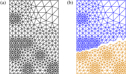
Figure 1: (a) The mesh network of Bern et al. [49]. (b) The best division into equal-sized parts found by the spectral partitioning algorithm based on the Laplacian matrix.

This then is the spectral partitioning method in its simplest form. It is not guaranteed to minimize $R$, but, particularly in cases where $\lambda_{2}$ is well separated from the eigenvalues above it, it often does very well. Figure 1 shows an example application typical of those found in the literature, to a two-dimensional mesh such as might be used in parallel finite-element calculations. This particular mesh is a small 547-vertex example from Bern et al. [49] and is shown complete in panel (a) of the figure. Panel (b) shows the division of the mesh into two parts of $273$ and $274$ vertices respectively using the spectral partitioning approach, which finds a cut of size 46 edges in this case.

Although the cut found in this example is a reasonable one, it does not appear—at least to this author’s eye—that the vertex groups in Fig. 1b constitute any kind of natural division of the network into “communities.” This is typical of the problems to which spectral partitioning is usually applied: in most circumstances the network in question does not divide up easily into groups of the desired sizes, but one must do the best one can. For these types of tasks, spectral partitioning is an effective and appropriate tool. The task of finding natural community divisions in a network, however, is quite different, and demands a different approach, as we now discuss.

III Community structure and modularity

Despite its evident success in the graph partitioning arena, spectral partitioning is a poor approach for detecting natural community structure in real-world networks, which is the primary topic of this paper. The issue is with the condition that the sizes of the groups into which the network is divided be fixed. This condition is neither appropriate nor realistic for community detection problems. In most cases we do not know in advance the sizes of the communities in a network and choosing arbitrary sizes will usually preclude us from finding the best solution to the problem. We would like instead to let the group sizes be free, but the spectral partitioning method breaks down if we do this, as we have seen: if the group sizes are not fixed, then the minimum cut size is always achieved by putting all vertices in one group and none in the other. Indeed, this statement is considerably broader than the spectral partitioning method itself, since any method that correctly minimizes the cut size without constraint on the group sizes is sure to find, in the general case, that the minimum value is achieved for this same trivial division.

Several approaches have been proposed to get around this problem. For instance, the ratio cut method [50] minimizes not the simple cut size $R$ but the ratio $R/(n_{1}n_{2})$, where $n_{1}$ and $n_{2}$ are again the sizes of the two groups of vertices. This penalizes configurations in which either of the groups is small and hence favors balanced divisions over unbalanced ones, releasing us from the obligation to fix the group sizes. Spectral algorithms based on ratio cuts have been proposed [51, 52] and have proved useful for certain classes of partitioning problems. Still, however, this approach effectively chooses the group sizes, at least approximately, since it is biased in favor of divisions into equal-sized parts. Variations are possible that are biased towards other, unequal part sizes, but then one must choose those parts sizes and so again we have a situation in which we need to know in advance the sizes of the groups if we are to get the “right” results. The ratio cut method does allow some leeway for the sizes to vary around their specified values, which makes it more flexible than the simple minimum cut method, but at its core it still suffers from the same drawbacks that make standard spectral partitioning inappropriate for community detection.

The fundamental problem with all of these methods is that cut sizes are simply not the right thing to optimize because they don’t accurately reflect our intuitive concept of network communities. A good division of a network into communities is not merely one in which the number of edges running between groups is small. Rather, it is one in which the number of edges between groups is smaller than expected. Only if the number of between-group edges is significantly lower than would be expected purely by chance can we justifiably claim to have found significant community structure. Equivalently, we can examine the number of edges within communities and look for divisions of the network in which this number is higher than expected—the two approaches are equivalent since the total number of edges is fixed and any edges that do not lie between communities must necessarily lie inside them.

These considerations lead us to shift our attention from measures based on pure cut size to a modified benefit function $Q$ defined by

$$Q =$$ (number of edges within communities) (17)

$$\quad{}-\mbox{(expected number of such edges)}.$$

This benefit function is called modularity [53, 18]. It is a function of the particular division of the network into groups, with larger values indicating stronger community structure. Hence we should, in principle, be able to find good divisions of a network into communities by optimizing the modularity over possible divisions. This approach, proposed in [24] and since pursued by a number of authors [38, 39, 8, 40, 32], has proven highly effective in practice [36] and is the primary focus of this article.

The first term in Eq. (17) is straightforward to calculate. The second, however, is rather vague and needs to be made more precise before we can evaluate the modularity. What exactly do we mean by the “expected number” of edges within a community? Answering this question is essentially equivalent to choosing a “null model” against which to compare our network. The definition of the modularity involves a comparison of the number of within-group edges in a real network and the number in some equivalent randomized model network in which edges are placed without regard to community structure.

It is one of the strengths of the modularity approach that it makes the role of this null model explicit and clear. All methods for finding communities are, in a sense, assuming some null model, since any method must make a value judgment about when a particular density of edges is significant enough to define a community. In most cases, this assumption is hidden within the workings of a computer algorithm and is difficult to disentangle, even when the algorithm itself is well understood. By bringing its assumptions out into the open, the modularity method gives us more control over our calculations and more understanding of their implications.

Our null model must have the same number of vertices $n$ as the original network, so that we can divide it into the same groups for comparison, but apart from this we have a good deal of freedom about our choice of model. We here consider the broad class of randomized models in which we specify separately the probability $P_{ij}$ for an edge to fall between every pair of vertices $i,j$. More precisely, $P_{ij}$ is the expected number of edges between $i$ and $j$, a definition that allows for the possibility that there may be more than one edge between a pair of vertices, which happens in certain types of networks. We will consider some particular choices of $P_{ij}$ in a moment, but for now let us pursue the developments in general form.

Given $P_{ij}$, the modularity can be defined as follows. The actual number of edges falling between a particular pair of vertices $i$ and $j$ is $A_{ij}$, Eq. (1), and the expected number is, by definition, $P_{ij}$. Thus the actual minus expected number of edges between $i$ and $j$ is $A_{ij}-P_{ij}$ and the modularity is (proportional to) the sum of this quantity over all pairs of vertices belonging to the same community. Let us define $g_{i}$ to be the community to which vertex $i$ belongs. Then the modularity can be written

$$Q={1\over 2m}\sum_{ij}\bigl{[}A_{ij}-P_{ij}\bigr{]}\delta(g_{i},g_{j}),$$ (18)

where $\delta(r,s)=1$ if $r=s$ and 0 otherwise and $m$ is again the number of edges in the network. The extra factor of $1/2m$ in Eq. (18) is purely conventional; it is included for compatibility with previous definitions of the modularity and plays no part in the maximization of $Q$ since it is a constant for any given network. A special case of Eq. (18) was given previously by the present author in [54] and independently, in slightly different form, by White and Smyth [55]. A number of other expressions for the modularity have also been presented by various authors [18, 39, 40] and are convenient in particular applications. Also of interest is the derivation of the modularity given recently by Reichardt and Bornholdt [34], which is quite general and provides an interesting alternative to the derivation presented here.

Returning to the null model, how should $P_{ij}$ be chosen? The choice is not entirely unconstrained. First, we consider in this paper only undirected networks, which implies that $P_{ij}=P_{ji}$. Second, it is axiomatically the case that $Q=0$ when all vertices are placed in a single group together: by definition, the number of edges within groups and the expected number of such edges are both equal to $m$ in this case. Setting all $g_{i}$ equal in Eq. (18), we find that $\sum_{ij}[A_{ij}-P_{ij}]=0$ or equivalently

$$\sum_{ij}P_{ij}=\sum_{ij}A_{ij}=2m.$$ (19)

This equation says that we are restricted to null models in which the expected number of edges in the entire network equals the actual number of edges in the original network—a natural choice if our comparison of numbers of edges within groups is to have any meaning.

Beyond these basic considerations, there are many possible choices of null model and several have been considered previously in the literature [18, 27, 56]. Perhaps the simplest is the standard (Bernoulli) random graph, in which edges appear with equal probability $P_{ij}=p$ between all vertex pairs. With a suitably chosen value of $p$ this model can be made to satisfy (19) but, as many authors have pointed out [57, 58, 59], the model is not a good representation of most real-world networks. A particularly glaring aspect in which it errs is its degree distribution. The random graph has a binomial degree distribution (or Poisson in the limit of large graph size), which is entirely unlike the right-skewed degree distributions found in most real-world networks [60, 61]. A much better null model would be one in which the degree distribution is approximately the same as that of the real-world network of interest. To satisfy this demand we will restrict our attention in this paper to models in which the expected degree of each vertex within the model is equal to the actual degree of the corresponding vertex in the real network. Noting that the expected degree of vertex $i$ is given by $\sum_{j}P_{ij}$, we can express this condition as

$$\sum_{j}P_{ij}=k_{i}.$$ (20)

If this constraint is satisfied, then (19) is automatically satisfied as well, since $\sum_{i}k_{i}=2m$.

Equation (20) is a considerably more stringent constraint than (19)—in most cases, for instance, it excludes the Bernoulli random graph—but it is one that we believe makes good sense, and one moreover that has a variety of desirable consequences for the developments that follow.

The simplest null model in this class, and the only one that has been considered at any length in the past, is the model in which edges are placed entirely at random, subject to the constraint (20). That is, the probability that an end of a randomly chosen edge attaches to a particular vertex $i$ depends only on the expected degree $k_{i}$ of that vertex, and the probabilities for the two ends of a single edge are independent of one another. This implies that the expected number of edges $P_{ij}$ between vertices $i$ and $j$ is the product $f(k_{i})f(k_{j})$ of separate functions of the two degrees, where the functions must be the same since $P_{ij}$ is symmetric. Then Eq. (20) implies

$$\sum_{j=1}^{n}P_{ij}=f(k_{i})\sum_{j=1}^{n}f(k_{j})=k_{i},$$ (21)

for all $i$ and hence $f(k_{i})=Ck_{i}$ for some constant $C$. And Eq. (19) says that

$$2m=\sum_{ij}P_{ij}=C^{2}\sum_{ij}k_{i}k_{j}=(2mC)^{2},$$ (22)

and hence $C=1/\sqrt{2m}$ and

$$P_{ij}={k_{i}k_{j}\over 2m}.$$ (23)

This model has been studied in the past in its own right as a model of a network, for instance by Chung and Lu [62]. It is also closely related to the configuration model, which has been studied widely in the mathematics and physics literature [63, 64, 65, 62]. Indeed, essentially all expected properties of our model and the configuration model are identical in the limit of large network size, and hence Eq. (23) can be considered equivalent to the configuration model in this limit.

Although many of the developments outlined in this paper are true for quite general choices of the null model used to define the modularity, the choice (23) is the only one we will pursue here. It is worth keeping mind however that other choices are possible: Massen and Doye [56], for instance, have used a variant of the configuration model in which multiedges and self-edges were excluded. And further choices could be useful in specific cases, such as cases where there are strong correlations between the degrees of vertices [66, 67] or where there is a high level of network transitivity [59].

IV Spectral optimization of modularity

Once we have an explicit expression for the modularity we can determine the community structure by maximizing it over possible divisions of the network. Unfortunately, exhaustive maximization over all possible divisions is computational intractable because there are simply too many divisions, but various approximate optimization methods have proven effective [24, 38, 39, 8, 56, 34, 40]. Here, we develop a matrix-based approach analogous to the spectral partitioning method of Section II, which leads not only to a whole array of possible optimization algorithms but also to new insights about the nature and implications of community structure in networks.

IV.1 Leading eigenvector method

As before, let us consider initially the division of a network into just two communities and denote a potential such division by an index vector $\mathbf{s}$ with elements as in Eq. (3). We notice that the quantity $\mbox{$\frac{1}{2}$}(s_{i}s_{j}+1)$ is 1 if $i$ and $j$ belong to the same group and 0 if they belong to different groups or, in the notation of Eq. (18),

$$\delta(g_{i},g_{j})=\mbox{$\frac{1}{2}$}(s_{i}s_{j}+1).$$ (24)

Thus we can write (18) in the form

$$Q = {1\over 4m}\sum_{ij}\bigl{[}A_{ij}-P_{ij}\bigr{]}(s_{i}s_{j}+1)$$ (25)

$$= {1\over 4m}\sum_{ij}\bigl{[}A_{ij}-P_{ij}\bigr{]}s_{i}s_{j},$$

where we have in the second line made use of Eq. (19). This result can conveniently be rewritten in matrix form as

$$Q={1\over 4m}\mathbf{s}^{T}\mathbf{B}\mathbf{s},$$ (26)

where $\mathbf{B}$ is the real symmetric matrix having elements

$$B_{ij}=A_{ij}-P_{ij}.$$ (27)

We call this matrix the modularity matrix and it plays a role in the maximization of the modularity equivalent to that played by the Laplacian in standard spectral partitioning: Equation (26) is the equivalent of Eq. (9) for the cut size and matrix methods can thus be applied to the modularity that are the direct equivalents of those developed for spectral partitioning, as we now show.

First, let us point out a few important properties of the modularity matrix. Equations (6) and (20) together imply that all rows (and columns) of the modularity matrix sum to zero:

$$\sum_{j}B_{ij}=\sum_{j}A_{ij}-\sum_{j}P_{ij}=k_{i}-k_{i}=0.$$ (28)

This immediately implies that for any network the vector $(1,1,1,\ldots)$ is an eigenvector of the modularity matrix with eigenvalue zero, just as is the case with the Laplacian. Unlike the Laplacian however, the eigenvalues of the modularity matrix are not necessarily all of one sign and in practice the matrix usually has both positive and negative eigenvalues. This observation—and the eigenspectrum of the modularity matrix in general—are, as we will see, closely tied to the community structure of the network.

Working from Eq. (26) we now proceed by direct analogy with Section II. We write $\mathbf{s}$ as a linear combination of the normalized eigenvectors $\mathbf{u}_{i}$ of the modularity matrix, $\mathbf{s}=\sum_{i=1}^{n}a_{i}\mathbf{u}_{i}$ with $a_{i}=\mathbf{u}_{i}^{T}\mathbf{s}$. Then

$$Q={1\over 4m}\sum_{i}a_{i}^{2}\beta_{i},$$ (29)

where $\beta_{i}$ is the eigenvalue of $\mathbf{B}$ corresponding to the eigenvector $\mathbf{u}_{i}$. We now assume that the eigenvalues are labeled in decreasing order $\beta_{1}\geq\beta_{2}\geq\ldots\geq\beta_{n}$ and the task of maximizing $Q$ is one of choosing the quantities $a_{i}^{2}$ so as to place as much as possible of the weight in the sum (29) in the terms corresponding to the largest (most positive) eigenvalues.

As with ordinary spectral partitioning, this would be a simple task if our choice of $\mathbf{s}$ were unconstrained (apart from normalization): we would just choose $\mathbf{s}$ proportional to the leading eigenvector $\mathbf{u}_{1}$ of the modularity matrix. But the elements of $\mathbf{s}$ are restricted to the values $s_{i}=\pm 1$, which means that $\mathbf{s}$ cannot normally be chosen parallel to $\mathbf{u}_{1}$. Again as before, however, good approximate solutions can be obtained by choosing $\mathbf{s}$ to be as close to parallel with $\mathbf{u}_{1}$ as possible, which is achieved by setting

$$s_{i}=\begin{cases}+1&\quad\text{if $u^{(1)}_{i}\geq 0$,}\\ -1&\quad\text{if $u^{(1)}_{i}<0$.}\end{cases}$$ (30)

This then is our first and simplest algorithm for community detection: we find the eigenvector corresponding to the most positive eigenvalue of the modularity matrix and divide the network into two groups according to the signs of the elements of this vector.

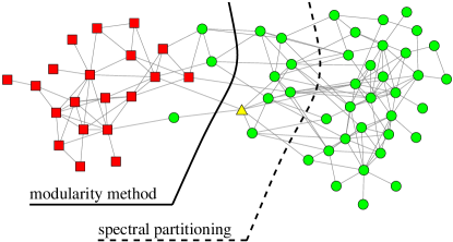
Figure 2: The dolphin social network of Lusseau et al. [68]. The dashed curve represents the division into two equally sized parts found by a standard spectral partitioning calculation (Section II). The solid curve represents the division found by the modularity-based method of this section. And the squares and circles represent the actual division of the network observed when the dolphin community split into two as a result of the departure of a keystone individual. (The individual who departed is represented by the triangle.)

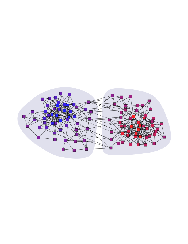
Figure 3: The network of political books described in the text. Vertex colors range from blue to red to represent the values of the corresponding elements of the leading eigenvector of the modularity matrix.

In practice, this method works nicely, as discussed in [32]. Making the choice (23) for our null model, we have applied it to a variety of standard and less standard test networks and find that it does a good job of finding community divisions. Figure 2 shows a representative example, an animal social network assembled and studied by Lusseau et al. [68]. The vertices in this network represent 62 bottlenose dolphins living in Doubtful Sound, New Zealand, with social ties between dolphin pairs established by direct observation over a period of several years. This network is of particular interest because, during the course of the study, the dolphin group split into two smaller subgroups following the departure of a key member of the population. The subgroups are represented by the shapes of the vertices in the figure. The dotted line denotes the division of the network into two equal-sized groups found by the standard spectral partitioning method. While, as expected, this method does a creditable job of dividing the network into groups of these particular sizes, it is clear to the eye that this is not the natural community division of the network and neither does it correspond to the division observed in real life. The spectral partitioning method is hamstrung by the requirement that we specify the sizes of the two communities; unless we know what they are in advance, blind application of the method will not usually find the “right” division of the network.

The method based on the leading eigenvector of the modularity matrix, however, does much better. Unconstrained by the need to find groups of any particular size, this method finds the division denoted by the solid line in the figure, which, as we see, corresponds quite closely to the split actually observed—all but three of the 62 dolphins are placed in the correct groups.

The magnitudes of the elements of the eigenvector $\mathbf{u}_{1}$ also contain useful information about the network, indicating, as discussed in [32], the “strength” with which vertices belong to the communities in which they are placed. As an example of this phenomenon consider Fig. 3, which depicts the network of political books from Ref. [32]. This network, compiled by V. Krebs (unpublished), represents recent books on US politics, with edges connecting pairs of books that are frequently purchased by the same customers of the on-line bookseller Amazon.com. Applying our method, we find that the network divides as shown in the figure, with the colors of the vertices representing the values of the elements of the eigenvector. The two groups correspond closely to the apparent alignment of the books according to left-wing and right-wing points of view [32], and are suggestively colored blue and red in the figure. The most blue and most red vertices are those that, by our calculation, belong most strongly to the two groups and are thus, perhaps, the “most left-wing” and “most right-wing” of the books under consideration. Those familiar with current US politics will be unsurprised to learn that the most left-wing book in this sense was the polemical Bushwacked by Molly Ivins and Lou Dubose. Perhaps more surprising is the most right-wing book: A National Party No More by Zell Miller.

IV.2 Other eigenvectors of the modularity matrix

The algorithm described in the previous section has two obvious shortcomings. First, it divides networks into only two communities, while real-world networks can certainly have more than two. Second, it makes use only of the leading eigenvector of the modularity matrix and ignores all the others, which throws away useful information contained in those other vectors. Both of these shortcomings are remedied by the following generalization of the method.

Consider the division of a network into $c$ non-overlapping communities, where $c$ may now be greater than 2. Following Alpert and Yao [69] and more recently White and Smyth [55], let us define an $n\times c$ index matrix $\mathbf{S}$ with one column for each community: $\mathbf{S}=(\mathbf{s}_{1}|\mathbf{s}_{2}|\ldots|\mathbf{s}_{c})$. Each column is an index vector now of $(0,1)$ elements (rather than $\pm 1$ as previously), such that

$$S_{ij}=\begin{cases}1&\quad\text{if vertex~{}$i$ belongs to community~{}$j$,}\\ 0&\quad\text{otherwise.}\end{cases}$$ (31)

Note that the columns of $\mathbf{S}$ are mutually orthogonal, that the rows each sum to unity, and that the matrix satisfies the normalization condition $\mathrm{Tr}(\mathbf{S}^{T}\mathbf{S})=n$.

Observing that the $\delta$-symbol in Eq. (18) is now given by

$$\delta(g_{i},g_{j})=\sum_{k=1}^{c}S_{ik}S_{jk},$$ (32)

the modularity for this division of the network is

$$Q=\sum_{i,j=1}^{n}\>\sum_{k=1}^{c}B_{ij}S_{ik}S_{jk}=\mathrm{Tr}(\mathbf{S}^{T}\mathbf{B}\mathbf{S}),$$ (33)

where here and henceforth we suppress the leading multiplicative constant $1/2m$ from Eq. (18), which has no effect on the position of the maximum of the modularity.

Writing $\mathbf{B}=\mathbf{U}\mathbf{D}\mathbf{U}^{T}$, where $\mathbf{U}=(\mathbf{u}_{1}|\mathbf{u}_{2}|\ldots)$ is the matrix of eigenvectors of $\mathbf{B}$ and $\mathbf{D}$ is the diagonal matrix of eigenvalues $D_{ii}=\beta_{i}$, we then find that

$$Q=\sum_{j=1}^{n}\sum_{k=1}^{c}\beta_{j}(\mathbf{u}_{j}^{T}\mathbf{s}_{k})^{2}.$$ (34)

Again we wish to maximize this modularity, but now we have no constraint on the number $c$ of communities; we can give $\mathbf{S}$ as many columns as we like in our effort to make $Q$ as large as possible.

If the elements of the matrix $\mathbf{S}$ were unconstrained apart from the basic conditions on the rows and columns mentioned above, a choice of $c$ communities would be equivalent to choosing $c-1$ independent, mutually orthogonal columns $\mathbf{s}_{1}\ldots\mathbf{s}_{c-1}$. (Only $c-1$ of the columns are independent, the last being fixed by the condition that the rows of $\mathbf{S}$ sum to unity.) In this case our path would be clear: $Q$ would be maximized by choosing the columns proportional to the leading eigenvectors of $\mathbf{B}$. However, only those eigenvectors corresponding to positive eigenvalues can give positive contributions to the modularity, so the optimal modularity would be achieved by choosing exactly as many independent columns of $\mathbf{S}$ as there are positive eigenvalues, or equivalently by choosing the number of groups $c$ to be 1 greater than the number of positive eigenvalues.

Unfortunately, our problem has the additional constraint that the index vectors $\mathbf{s}_{i}$ have only binary $(0,1)$ elements, which means it may not be possible to find as many index vectors making positive contributions to the modularity as the set of positive eigenvalues suggests. Thus the number of positive eigenvalues, plus 1, is an upper bound on the number of communities and again we see that there is an intimate connection between the properties of the modularity matrix and the community structure of the network it describes.

IV.3 Vector partitioning algorithm

In Section IV.1 we maximized the modularity approximately by focusing solely on the term in $Q$ proportional to the largest eigenvalue of $\mathbf{B}$. Let us now make the more general (and often better) approximation of keeping the leading $p$ eigenvalues, where $p$ may be anywhere between 1 and $n$. Some of the eigenvalues, however, may be negative, which will prove inconvenient. To get around this we rewrite Eq. (33) thus:

$$Q = n\alpha+\mathrm{Tr}[\mathbf{S}^{T}\mathbf{U}(\mathbf{D}-\alpha\mathbf{I})\mathbf{U}^{T}\mathbf{S}]$$ (35)

$$= n\alpha+\sum_{j=1}^{n}\sum_{k=1}^{c}(\beta_{j}-\alpha)\biggl{[}\sum_{i=1}^{n}U_{ij}S_{ik}\biggr{]}^{2},$$

where $\alpha$ is a constant whose value we will choose shortly and we have made use of $\mathrm{Tr}(\mathbf{S}^{T}\mathbf{S})=n$ and the fact that $\mathbf{U}$ is orthogonal.

Now, employing an argument similar to that used for ordinary spectral partitioning in [69], let us define a set of vertex vectors $\mathbf{r}_{i}$, $i=1\ldots n$, of dimension $p$, such that the $j$th component of the $i$th vector is

$$\bigl{[}\mathbf{r}_{i}\bigr{]}_{j}=\sqrt{\beta_{j}-\alpha}\,U_{ij}.$$ (36)

Provided we choose $\alpha\leq\beta_{p}$, $\mathbf{r}_{i}$ is guaranteed real for all $i$. Then, dropping terms in (35) proportional to the smallest $n-p$ of the factors $\beta_{j}-\alpha$, we have

$$Q \simeq n\alpha+\sum_{j=1}^{p}\sum_{k=1}^{c}\biggl{[}\sum_{i=1}^{n}\sqrt{\beta_{j}-\alpha}\,U_{ij}S_{ik}\biggr{]}^{2}$$ (37)

$$= n\alpha+\sum_{k=1}^{c}\sum_{j=1}^{p}\biggl{[}\sum_{i\in G_{k}}\bigl{[}\mathbf{r}_{i}\bigr{]}_{j}\biggr{]}^{2}$$

$$= n\alpha+\sum_{k=1}^{c}|\mathbf{R}_{k}|^{2},\qquad{}$$

where $G_{k}$ is the set of vertices comprising group $k$ and the community vectors $\mathbf{R}_{k}$, $k=1\ldots c$, are

$$\mathbf{R}_{k}=\sum_{i\in G_{k}}\mathbf{r}_{i}.$$ (38)

The community structure problem is now equivalent to choosing a division of the vertices into groups so as to maximize the magnitudes of the vectors $\mathbf{R}_{k}$. This means we need to arrange that the individual vertex vectors $\mathbf{r}_{i}$ going into each group point in approximately the same direction. Problems of this type are called vector partitioning problems.

The parameter $p$ controls the balance between the complexity of the vector partitioning problem and the accuracy of the approximation we make by keeping only some of the eigenvalues. The calculations will be faster but less accurate for smaller $p$ and slower but more accurate for larger. For the special case $p=n$ where we keep all of the eigenvalues, Eq. (37) is exact. In this case, we note that the vertex vectors have the property

$$\mathbf{r}_{i}^{T}\mathbf{r}_{j}=\sum_{k=1}^{n}U_{ik}(\beta_{k}-\alpha)U_{jk}=B_{ij}-\alpha\delta_{ij}.$$ (39)

It’s then simple to see that Eq. (37) is trivially equivalent to the fundamental definition (18) of the modularity, so in the $p=n$ case our mapping to a vector partitioning problem gives little insight into the modularity maximization problem. The real advantage of our approach comes when $p<n$, where the method extracts precisely those factors that make the principal contributions to the modularity—i.e., those corresponding to the largest eigenvalues—discarding those that have relatively little effect. In practice, as we have seen for the single-eigenvector algorithm, the main features of the community structure are often captured by just the first eigenvector or perhaps the first few, which allows us to reduce the complexity of our optimization problem immensely.

The approach is similar in concept to the standard technique of principal components analysis (PCA) used to reduce high-dimensional data sets to manageably small dimension by focusing on the eigendirections along which the variance about the mean is greatest and ignoring directions that contribute little. In fact, this similarity is more than skin-deep: the form of our modularity matrix is closely analogous to the covariance matrix whose eigenvectors are the basis for PCA. The elements of the covariance matrix are correlation functions of the form $\langle xy\rangle-\langle x\rangle\langle y\rangle$, where $x$ and $y$ denote measured variables in the data set. Thus the covariance is the difference between the actual value of the mean product $\langle xy\rangle$ of two variables and the value $\langle x\rangle\langle y\rangle$ expected by chance for that product if the variables were uncorrelated. Similarly, the elements $B_{ij}=A_{ij}-k_{i}k_{j}/2m$ of the modularity matrix are equal to the actual number of edges $A_{ij}$ between a given pair of vertices minus the number $k_{i}k_{j}/2m$ expected by chance, expressed in a product form. In a sense, our spectral method for modularity optimization can be regarded as a “principal components analysis for networks.” This aspect of the method is clear, for instance, in the study of political books represented in Fig. 3: the leading eigenvector used to assign the colors to the vertices in the figure is playing a role equivalent to the eigendirections in PCA, defining a “direction of greatest variation” in the structure of the network. The vertex vectors of Eq. (36) are similarly analogous to the low-dimensional projections used in PCA.

Returning to our algorithm, let us consider again the special case of the division of a network into just two communities. (Multi-way division is considered in Section VI.) Since $(1,1,1,\ldots)$ is always an eigenvector of the modularity matrix and the eigenvectors are orthogonal, the elements of all other eigenvectors must sum to zero:

$$\sum_{i=1}^{n}\bigl{[}\mathbf{u}_{j}\bigr{]}_{i}=\sqrt{n}\,\mathbf{u}_{1}^{T}\mathbf{u}_{j}=0.$$ (40)

But Eq. (36) then implies that

$$\sum_{i=1}^{n}\bigl{[}\mathbf{r}_{i}\bigr{]}_{j}=\sqrt{\beta_{j}-\alpha}\sum_{i=1}^{n}U_{ij}=\sqrt{\beta_{j}-\alpha}\sum_{i=1}^{n}\bigl{[}\mathbf{u}_{j}\bigr{]}_{i}=0,$$ (41)

and hence

$$\sum_{i=1}^{n}\mathbf{r}_{i}=0$$ (42)

for any value of $p$. This in turn implies that the community vectors $\mathbf{R}_{k}$ also sum to zero:

$$\sum_{k=1}^{c}\mathbf{R}_{k}=\sum_{k=1}^{c}\>\sum_{i\in G_{k}}\mathbf{r}_{i}=\sum_{i=1}^{n}\mathbf{r}_{i}=0.$$ (43)

And as a special case of this last result, any division of a network into two communities has community vectors $\mathbf{R}_{1}$ and $\mathbf{R}_{2}$ that are of equal magnitude and oppositely directed.

Furthermore, the maximum of the modularity, Eq. (37), is always achieved when each individual vertex vector $\mathbf{r}_{i}$ has a positive inner product with the community vector of the community to which the vertex belongs. To see this, observe that removing a vertex $i$ from a community $k$ where $\mathbf{R}_{k}\cdot\mathbf{r}_{i}<0$ produces a change in the corresponding term $|\mathbf{R}_{k}|^{2}$ in Eq. (37) of

$$|\mathbf{R}_{k}-\mathbf{r}_{i}|^{2}-|\mathbf{R}_{k}|^{2}=|\mathbf{r}_{i}|^{2}-2\mathbf{R}_{k}\cdot\mathbf{r}_{i}>0.$$ (44)

Similarly adding vertex $i$ to a community for which $\mathbf{R}_{k}\cdot\mathbf{r}_{i}>0$ also increases $|\mathbf{R}_{k}|^{2}$. Hence, we can always increase the modularity by moving vertices until they are in groups such that $\mathbf{R}_{k}\cdot\mathbf{r}_{i}>0$.

Taken together, these results imply that possible candidates for the optimal division of a network into two groups are fully specified by just the direction of the single vector $\mathbf{R}_{1}$. Once we have this direction, we know that the vertices divide according to whether their projection along this direction is positive or negative. Alternatively, we can consider the direction of $\mathbf{R}_{1}$ to define a perpendicular plane through the origin in the $p$-dimensional vector space occupied by the vertex vectors $\mathbf{r}_{i}$. The vertices then divide according to which side of this plane their vectors fall on. Finding the maximum of the modularity is then a matter of choosing this bisecting plane to maximize the magnitude of $\mathbf{R}_{1}$.

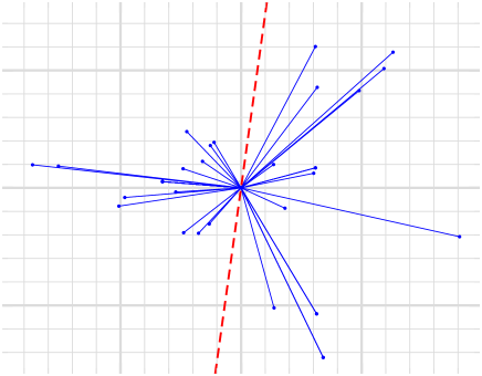
Figure 4: A plot of the vertex vectors $\mathbf{r}_{i}$ for a small network with $p=2$. The dotted line represents one of the $n$ possible topologically distinct cut planes.

In general, this still leaves us with a moderately difficult optimization problem: the number of bisecting planes that give distinct partitions of the vertex vectors is large and difficult to enumerate as the dimension $p$ of the space becomes large. For the case $p=2$, however, a relatively simple solution exists. Consider Fig. 4, which shows a typical example of the vertex vectors. In this two-dimensional case, there are only $n$ topologically distinct choices of the bisecting plane (actually just a line in this case, denoted by the dashed line in the figure), and furthermore the divisions of the vertices that these choices represent change by only a single vertex at a time as we rotate the plane about the origin. This makes it computationally simple to perform the rotation, keep track of the value of $\mathbf{R}_{1}$, and so find the maximum of the modularity within this approximation. Evaluating the magnitude of $\mathbf{R}_{1}$ involves a constant number of operations each time we move the line, and hence the total work involved in finding the maximum is $\mathrm{O}(n)$ for all $n$ possible positions, which is the same as the $\mathrm{O}(n)$ operations needed to separate the vertices in the $p=1$ case.

For $p>2$, we do not know of an efficient method to enumerate exhaustively all topologically distinct bisecting planes in the vertex vector space, and hence we have to turn to approximate methods for solving the vector partitioning problem. A number of reasonable heuristics have been described in the past. We have found acceptable though not spectacular results, for instance, with the “MELO” algorithm of [69], which is essentially a greedy algorithm in which a grouping of vectors is built up by repeatedly adding to it the vector that makes the largest contribution to $Q$.

IV.4 Choice of $\alpha$

Before implementing any of these methods, a crucial question we must answer is what value we should choose for the parameter $\alpha$. By tuning this value we can improve the accuracy of our approximation to $Q$ as follows.

By dropping the $n-p$ most negative eigenvalues, we are in effect making an approximation to the matrix $\mathbf{B}-\alpha\mathbf{I}$ in which it takes not its full value $\mathbf{U}(\mathbf{D}-\alpha\mathbf{I})\mathbf{U}^{T}$, but an approximate value $\mathbf{U}(\mathbf{D}^{\prime}-\alpha\mathbf{I}^{\prime})\mathbf{U}^{T}$, where $\mathbf{D}^{\prime}$ and $\mathbf{I}^{\prime}$ are the matrices $\mathbf{D}$ and $\mathbf{I}$ with the last $n-p$ diagonal elements set to zero. We can quantify the error this introduces by calculating the sum of the squares of the elements of the difference between the two matrices, which is given by

$$\chi^{2} = \mathrm{Tr}[\mathbf{U}(\mathbf{D}-\alpha\mathbf{I})\mathbf{U}^{T}-\mathbf{U}(\mathbf{D}^{\prime}-\alpha\mathbf{I}^{\prime})\mathbf{U}^{T}]^{2}$$ (45)

$$= \mathrm{Tr}[(\mathbf{D}-\alpha\mathbf{I})-(\mathbf{D}^{\prime}-\alpha\mathbf{I}^{\prime})]^{2}=\!\!\sum_{i=p+1}^{n}(\beta_{i}-\alpha)^{2},\qquad{}$$

where in the second line we have made use of the fact that $\mathbf{U}$ is orthogonal.

Minimizing this error by setting the derivative $\mathrm{d}\chi^{2}/\mathrm{d}\alpha=0$, we find

$$\alpha={1\over n-p}\sum_{i=p+1}^{n}\beta_{i}.$$ (46)

In other words, the minimal mean square error introduced by our approximation is achieved by setting $\alpha$ equal to the mean of the eigenvalues that have been dropped. The only exception is when $p=n$, where the choice of $\alpha$ makes no difference since no approximation is being made anyway. In our calculations we have used $\alpha=\beta_{n}$ in this case, but any choice $\alpha\geq\beta_{n}$ would work equally well.

V Implementation

Implementation of the methods described in Section IV is straightforward. The leading-eigenvector method of Section IV.1 requires us to find only the single eigenvector of the modularity matrix $\mathbf{B}$ corresponding to the most positive eigenvalue. This is most efficiently achieved by the direct multiplication or power method. Starting with a trial vector, we repeatedly multiply by the modularity matrix and—unless we are unlucky enough to have chosen another eigenvector as our trial vector—the result will converge to the eigenvector of the matrix having the eigenvalue of largest magnitude. In some cases this eigenvalue will be the most positive one, in which case our calculation ends at this point. In other cases the eigenvalue of largest magnitude may be negative. If this happens then, denoting this eigenvalue by $\beta_{n}$, we calculate the shifted matrix $\mathbf{B}-\beta_{n}\mathbf{I}$, which has eigenvalues $\beta_{i}-\beta_{n}$ (necessarily all nonnegative) and the same eigenvectors as the modularity matrix itself. Then we repeat the power-method calculation for this new matrix and this time the eigenvalue of largest magnitude must be $\beta_{1}-\beta_{n}$ and the corresponding eigenvector is the one we are looking for.

For the method of Section IV.2, we require either all of the eigenvectors of the modularity matrix or a subset corresponding to the $p$ most positive eigenvalues. These are most conveniently calculated using the Lanczos method or one of its variants [70]. The fundamental matrix operation at the heart of the Lanczos method is again multiplication of the matrix $\mathbf{B}$ into a trial vector.

Efficient implementation of any of these methods thus rests upon our ability to rapidly multiply an arbitrary vector $\mathbf{x}$ by the modularity matrix. This presents a problem because the modularity matrix is dense, and hence it appears that matrix multiplications will demand $\mathrm{O}(n^{2})$ time each, where $n$ is, as before, the number of vertices in the network (which is also the size of the matrix). By contrast, the equivalent calculation in standard spectral partitioning is much faster because the Laplacian matrix is sparse, having only $\mathrm{O}(n+m)$ nonzero elements, where $m$ is the number of edges in the network.

For the standard choice, Eq. (23), of null model used to define the modularity, however, it turns out that we can multiply by the modularity matrix just as fast as by the Laplacian by making use of the special structure of the matrix. In vector notation the modularity matrix can in this case be written

$$\mathbf{B}=\mathbf{A}-{\mathbf{k}\mathbf{k}^{T}\over 2m},$$ (47)

where $\mathbf{A}$ is the adjacency matrix, Eq. (1), and $\mathbf{k}$ is the $n$-element vector whose elements are the degrees $k_{i}$ of the vertices. Then

$$\mathbf{B}\mathbf{x}=\mathbf{A}\mathbf{x}-{\mathbf{k}^{T}\mathbf{x}\over 2m}\,\mathbf{k}.$$ (48)

Since the adjacency matrix is sparse, having only $\mathrm{O}(m)$ elements, the first term can be evaluated in $\mathrm{O}(m)$ time, while the second requires us to evaluate the inner product $\mathbf{k}^{T}\mathbf{x}$ only once and then multiply it into each element of $\mathbf{k}$ in turn, both operations taking $\mathrm{O}(n)$ time. Thus the entire matrix multiplication can be completed in $\mathrm{O}(m+n)$ time, just as with the normal Laplacian matrix. If a shift of the eigenvalues is required to find the most positive one, as described above, then there is an additional term $-\beta_{n}\mathbf{I}$ in the matrix, but this also can be multiplied into an arbitrary vector in $\mathrm{O}(n)$ time, so again the entire operation can be completed in $\mathrm{O}(m+n)$ time.

Typically $\mathrm{O}(n)$ matrix multiplications are required for either the power method or the Lanczos method to converge to the required eigenvalues, and hence the calculation takes $\mathrm{O}((m+n)n)$ time overall. In the common case in which the network is sparse and $m\propto n$, this simplifies to $\mathrm{O}(n^{2})$.

While this is, essentially, the end of the calculation for the power method, the Lanczos method unfortunately demands more effort to find the eigenvectors themselves. In fact, it takes $\mathrm{O}(n^{3})$ time to find all eigenvectors of a matrix using the Lanczos method, which is quite slow. There are on the other hand variants of the Lanczos method (as well as other methods entirely) that can find just a few leading eigenvectors faster than this, which makes calculations that focus on a fixed small number of eigenvectors preferable to ones that use all eigenvectors. In our calculations we have primarily concentrated on algorithms that use only one or two eigenvectors, which typically run in time $\mathrm{O}(n^{2})$ on a sparse network.

V.1 Refinement of the modularity

The methods for spectral optimization of the modularity described in Section IV are only approximate. Indeed, the problem of modularity optimization is formally equivalent to an instance of the NP-hard MAX-CUT problem, so it is almost certainly the case that no polynomial-time algorithm exists that will find the modularity optimum in all cases. Given that the algorithms we have described run in polynomial time, it follows that they must fail to find the optimum in some cases, and hence that there is room for improvement of the results.

In standard graph partitioning applications it is common to use a spectral approach based on the graph Laplacian as a first pass at the problem of dividing a network. The spectral method gives a broad picture of the general shape the division should take, but there is often room for improvement. Typically another algorithm, such as the Kernighan–Lin algorithm [71], which swaps vertex pairs between groups in an effort to reduce the cut size, is used to refine this first pass, and the resulting two-stage joint strategy gives considerably better results than either stage on its own.

We have found that a similar joint strategy gives good results in the present case also: the divisions found with our spectral approach can be improved in small but significant ways by adding a refinement step akin to the Kernighan–Lin algorithm. As described in [32], we take an initial division into two communities derived, for instance, from the leading-eigenvector method of Section IV.1 and move single vertices between the communities so as to increase the value of the modularity as much as possible, with the constraint that each vertex can be moved only once. Repeating the whole process iteratively until no further improvement is obtained, we find a final value of the modularity which can improve on that derived from the spectral method alone by tens of percent in some cases, and smaller but still significant amounts in other cases. Although the absolute gains in modularity are not always large, we find that this refinement step is very much worth the effort it entails, raising the typical level of performance of our methods from the merely good to the excellent, when compared with other algorithms. Specific examples are given in [32].

It is certainly possible that other refinement strategies might also give good results. For instance, the “extremal optimization” method explored by Duch and Arenas [40] for optimizing modularity could be employed as a refinement method by using the output of our spectral division as its starting point, rather than the random configuration used as a starting point by Duch and Arenas.

VI Dividing networks into more than two communities

So far we have discussed primarily methods for dividing networks into two communities. Many of the networks we are concerned with, however, have more than two communities. How can we generalize our methods to this case? The simplest approach is repeated division into two. That is, we use one of the methods described above to divide our network in two and then divide those parts in two again, and so forth. This approach was described briefly in Ref. [32].

It is important to appreciate that upon further subdividing a community within a network into two parts, the additional contribution $\Delta Q$ to the modularity made by this subdivision is not given correctly if we apply the algorithms of Section IV to that community alone. That is, we cannot simply write down the modularity matrix for the community in question considered as a separate graph in its own right and examine the leading eigenvector or eigenvectors. Instead we proceed as follows. Let us denote the set of vertices in the community to be divided by $G$ and let $n_{G}$ be the number of vertices within this community. Now let $\mathbf{S}$ be an $n_{G}\times c$ index matrix denoting the subdivision of the community into $c$ subcommunities such that

$$S_{ij}=\begin{cases}1&\quad\text{if vertex~{}$i$ belongs to subcommunity~{}$j$,}\\ 0&\quad\text{otherwise.}\end{cases}$$ (49)

Then, following Eq. (33), $\Delta Q$ is the difference between the modularities of the network before and after subdivision of the community thus:

$$\Delta Q = \sum_{i,j\in G}\>\sum_{k=1}^{c}B_{ij}S_{ik}S_{jk}-\sum_{i,j\in G}B_{ij}$$ (50)

$$= \sum_{k=1}^{c}\>\sum_{i,j\in G}\biggl{[}B_{ij}-\delta_{ij}\sum_{l\in G}B_{il}\biggr{]}S_{ik}S_{jk}$$

$$= \mathrm{Tr}(\mathbf{S}^{T}\mathbf{B}^{(G)}\mathbf{S}),$$

where $\mathbf{B}^{(G)}$ is an $n_{G}\times n_{G}$ generalized modularity matrix with elements indexed by the vertex labels $i,j$ of the vertices within group $G$ and having values

$$B^{(G)}_{ij}=B_{ij}-\delta_{ij}\sum_{l\in G}B_{il},$$ (51)

with $B_{ij}$ defined by Eq. (27).

Equation (50) has the same form as our previous expression, Eq. (33), for the modularity of the full network, and, following the same argument as for Eqs. (35) to (38), we can then show that optimization of the additional modularity contribution from subdivision of a community can also be expressed as a vector partitioning problem, just as before. We can approximate this vector partitioning problem using only the leading eigenvector as in Section IV.1 or using more than one vector as in Section IV.2. The resulting divisions can also be optimized using a “refinement” stage as in Section V.1, to find the best possible modularity at each step.

Using this method we can repeatedly subdivide communities to partition networks into smaller and smaller groups of vertices and in principle this process could continue until the network is reduced to $n$ communities containing only a single vertex each. Normally, however, we stop before this point is reached because there is no point in subdividing a community any further if no subdivision exists that will increase the modularity of the network as a whole. The appropriate strategy is to calculate explicitly the modularity contribution $\Delta Q$ at each step in the subdivision of a network, and to decline to subdivide any community for which the value of $\Delta Q$ is not positive. Communities with the property of having no subdivision that gives a positive contribution to the modularity of the network as a whole we call indivisible; the strategy described here is equivalent to subdividing communities repeatedly until every remaining community is indivisible.

This strategy appears to work very well in practice. It is, however, not perfect (a conclusion we could draw under any circumstances from the fact that it runs in polynomial time—see above). In particular, it is certain that repeated subdivision of a network into two parts will in some cases fail to find the optimal modularity configuration. Consider, for example, the (rather trivial) network shown in Fig. 5, which consists of eight vertices connected together in a line. By exhaustive enumeration we can show that, among possible divisions of this network into only two parts, the division indicated in Fig. 5a, right down the middle of the line, is the one that gives the highest modularity. The optimum modularity over divisions into any number of parts, however, is achieved for the three-way division shown in Fig. 5b. It is clear that if we first split the network as shown in Fig. 5a, no subsequent subdivision of the network can ever find the configuration of Fig. 5b, and hence our algorithm will fail in this case to find the global optimum. Nonetheless, the algorithm does appear to find divisions that are close to optimal in most cases we have investigated.

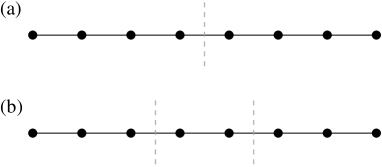
Figure 5: Division by the method of optimal modularity of a simple network consisting of eight vertices in a line. (a) The optimal division into just two parts separates the network symmetrically into two groups of four vertices each. (b) The optimal division into any number of parts divides the network into three groups as shown here.

Repeated subdivision is the approach we have taken to multi-community divisions in our own work, but it is not the only possible approach. In some respects a more satisfying approach would be to work directly from the expression (37) for the modularity of the complete network with a multi-community division. Unfortunately, maximizing (37) requires us to perform a vector partitioning into more than two groups, a problem about whose solution rather little is known. Some general observations are, however, worth making. First, we note that the community vectors $\mathbf{R}_{k}$ in the optimal solution of a vector partitioning problem always have directions more than $90^{\circ}$ apart. To demonstrate this, we note that the change in the contribution to Eq. (37) if we amalgamate two communities into one is

$$\bigl{|}\mathbf{R}_{1}+\mathbf{R}_{2}\bigr{|}^{2}-\bigl{(}\bigl{|}\mathbf{R}_{1}\bigr{|}^{2}+\bigl{|}\mathbf{R}_{2}\bigr{|}^{2}\bigr{)}=2\mathbf{R}_{1}\cdot\mathbf{R}_{2},$$ (52)

which is positive if the directions of $\mathbf{R}_{1}$ and $\mathbf{R}_{2}$ are less than $90^{\circ}$ apart. Thus we can always increase the modularity by amalgamating a pair of communities unless their vectors are more than $90^{\circ}$ apart.

But the maximum number of directions more than $90^{\circ}$ apart that can exist in a $p$-dimensional space is $p+1$, which means that $p+1$ is also the maximum number of communities we can find by optimizing a $p$-dimensional spectral approximation to the modularity. Thus if we use only a single eigenvector we will find at most two groups; if we use two we will find at most three groups, and so forth. So the choice of how many eigenvectors $p$ to work with is determined to some extent by the network: if the overall optimum modularity is for a division into $c$ groups, we will certainly fail to find that optimum if we use less than $c-1$ eigenvectors.

Second, we note that while true multi-way vector partitioning may present problems, simple heuristics that group the vertex vectors together can still produce good results. For instance, White and Smyth [55] have applied the standard technique of $k$-means clustering based on group centroids to a different but related optimization problem and have found good results. It is possible this approach would work for our problem also if applied to the centroids of the end-points of the vertex vectors. It is also possible that an intrinsically vector-based variant of $k$-means clustering could be created to tackle the vector partitioning problem directly, although we are not aware of such an algorithm in the current vector partitioning literature.

VII Negative eigenvalues and bipartite structure

It is clear from the developments of the previous sections that there is useful information about the structure of a network stored in the eigenvectors corresponding to the most positive eigenvalues of the modularity matrix. It is natural to ask whether there is also useful information in the eigenvectors corresponding to the negative eigenvalues and indeed it turns out that there is: the negative eigenvalues and their eigenvectors contain information about a nontrivial type of “anti-community structure” that is of substantial interest in some instances.

Consider again the case in which we divide our network into just two groups and look once more at Eq. (29), which gives the modularity in this case. Suppose now that instead of maximizing the terms involving the most positive eigenvalues, we maximize the terms involving the most negative ones. As we can easily see from the equation, this is equivalent to minimizing rather than maximizing the modularity.

What effect will this have on the divisions of the network that we find? Large negative values of the modularity correspond to divisions in which the number of edges within groups is smaller than expected on the basis of chance, and the number of edges between groups correspondingly bigger. Figure 6 shows a sketch of a network having this property. Such networks are said to be bipartite if there are no edges at all within groups, or approximately bipartite if there are a few within-group edges as in the figure. Bipartite or approximately bipartite graphs have attracted some attention in the recent literature. For instance, Kleinberg [72] has suggested that small bipartite subgraphs in the web graph may be a signature of so-called hub/authority structure within web communities, while Holme et al. [73] and Estrada and Rodríguez-Velázquez [74] have independently devised measures of bipartitivity and used them to analyze a variety of real-world networks.

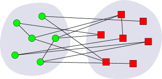
Figure 6: A small example of an approximately bipartite network. The network is composed of two groups of vertices and most edges run between vertices in different groups.

The arguments above suggest that we should be able to detect bipartite or approximately bipartite structure in networks by looking for divisions of the vertices that minimize modularity. In the simplest approximation, we can do this by focusing once more on just a single term in Eq. (29), that corresponding to the most negative eigenvalue $\beta_{n}$, and maximizing the coefficient of this eigenvalue by choosing $s_{i}=-1$ for vertices having a negative element in the corresponding eigenvector and $s_{i}=+1$ for the others. In other words, we can achieve an approximation to the minimum modularity division of the network by dividing vertices according to the signs of the elements in the eigenvector $\mathbf{u}_{n}$, and this division should correspond roughly to the most nearly bipartite division. We can also append a “refinement” step to the calculation, similar to that described in Section V.1, in which, starting from the division given by the eigenvector, we move single vertices between groups in an effort to minimize the modularity further.

As an example of this type of calculation, consider Fig. 7, which shows a network representing juxtapositions of words in a corpus of English text, in this case the novel David Copperfield by Charles Dickens. To construct this network, we have taken the 60 most commonly occurring nouns in the novel and the 60 most commonly occurring adjectives. (The limit on the number of words is imposed solely to permit a clear visualization; there is no reason in principle why the analysis could not be extended to a much larger network.) The vertices in the network represent words and an edge connects any two words that appear adjacent to one another at any point in the book. Eight of the words never appear adjacent to any of the others and are excluded from the network, leaving a total of 112 vertices.

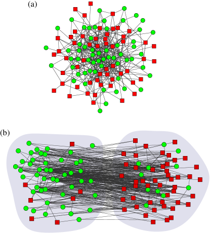
Figure 7: (a) The network of commonly occurring English adjectives (circles) and nouns (squares) described in the text. (b) The same network redrawn with the nodes grouped so as to minimize the modularity of the grouping. The network is now revealed to be approximately bipartite, with one group consisting almost entirely of adjectives and the other of nouns.

Typically adjectives occur next to nouns in English. It is possible for adjectives to occur next to other adjectives (“the big green bus”) or for nouns to occur next to other nouns (“the big tour bus”), but these juxtapositions are less common. Thus we would expect our network to be approximately bipartite in the sense described above: edges should run primarily between vertices representing different types of words, with fewer edges between vertices of the same type. One would be hard pressed to tell this from Fig. 7a, however: the standard layout algorithm used to draw the network completely fails to reveal the structure present. Figure 7b shows what happens when we divide the vertices by minimizing the modularity using the method described above—a first division according to the elements of the eigenvector with the most negative eigenvalue, followed by a refinement stage to reduce the modularity still further. It is now clear that the network is in fact nearly bipartite, and the two groups found by the algorithm correspond closely to the known groups of adjectives and nouns, as indicated by the shapes of the vertices. 83% of the words are classified correctly by this simple calculation.

Divisions with large negative modularity are—like those with large positive modularity—not limited to having only two groups. If we are interested purely in minimizing the modularity we can in principle use as many groups as we like to achieve that goal. A division with $k$ groups is called $k$-partite if edges run only between groups and approximately $k$-partite if there are a few within-group edges. One might imagine that one could find $k$-partite structure in a network just by looking for divisions that minimize the number of within-group edges, but brief reflection persuades us that the optimum solution to this search problem is always to put each vertex in a group on its own, which automatically means that all edges lie between groups and none within groups. As with the ordinary community structure problem, the way to avoid this trivial solution is to concentrate not on the total number of edges within groups but on the difference between this number and the expected number of such edges. Thus, once again, we are led naturally to the consideration of modularity as a measure of the best way to divide a network.

One way to minimize modularity over divisions into an arbitrary number of groups is to proceed by analogy with our earlier calculations of community structure and repeatedly divide the network in two using the single-eigenvector method above. Just as before, Eq. (50) gives the additional change $\Delta Q$ in the modularity upon subdivision of a group in a network, and the division process ends when the algorithm fails to find any subdivision with $\Delta Q<0$. Alternatively, one can derive the analog of Eq. (37) and thereby map the minimization of the modularity onto a vector partitioning problem. The appropriate definition of the vertex vectors turns out to be

$$\bigl{[}\mathbf{r}_{i}\bigr{]}_{j}=\sqrt{\alpha-\beta_{n+1-j}}\,U_{i,n+1-j},$$ (53)

where $\alpha$ is a constant chosen sufficiently large as to make $\alpha-\beta_{j}\geq 0$ for all terms in the sum that we keep. Then the modularity is given by

$$Q=n\alpha-\sum_{k=1}^{c}|\mathbf{R}_{k}|^{2},$$ (54)

with the community vectors $\mathbf{R}_{k}$ defined according to Eq. (38).

VIII Other uses of the modularity matrix

One of the striking properties of the Laplacian matrix is that, as described in Section II, it arises repeatedly in various different areas of graph theory. It is natural to ask whether the modularity matrix also crops up in other areas. In this section we describe briefly two other situations in which the modularity matrix appears, although neither has been viewed in terms of this matrix in the past, as far as we are aware.

VIII.1 Network correlations

For our first example, suppose we have a quantity $x_{i}$ defined on the vertices $i=1\ldots n$ of a network, such as degrees of vertices, ages of people in a social network, numbers of hits on web pages, and so forth. And let $\mathbf{x}$ be the $n$-component vector whose elements are the $x_{i}$. Then consider the quantity

$$r={1\over 2m}\mathbf{x}^{T}\mathbf{B}\mathbf{x},$$ (55)

where here we will take the same definition (23) for our null model that we have been using throughout. Observing that $\sum_{ij}A_{ij}=\sum_{i}k_{i}=2m$, we can rewrite $r$ as

$$r = {1\over 2m}\sum_{ij}\biggl{[}A_{ij}-{k_{i}k_{j}\over 2m}\biggr{]}x_{i}x_{j}$$ (56)

$$= {\sum_{ij}A_{ij}x_{i}x_{j}\over\sum_{ij}A_{ij}}-\Biggl{[}{\sum_{ij}A_{ij}x_{i}\over\sum_{ij}A_{ij}}\Biggr{]}^{2}.$$

Note that the ratios appearing in the second line are simply averages over all edges in the network, and hence $r$ has the form $\langle x_{i}x_{j}\rangle-\langle x_{i}\rangle\langle x_{j}\rangle$ of a correlation function measuring the correlation of the values $x_{i}$ over all pairs of vertices joined by an edge in the network.

Correlation functions of exactly this type have been considered previously as measures of so-called “assortative mixing,” the tendency for adjacent vertices in networks to have similar properties [67, 53]. For example, if the quantity $x_{i}$ is just the degree $k_{i}$ of a vertex, then $r$ is the covariance of the degrees of adjacent vertices, which takes positive values if vertices tend to have similar degrees to their neighbors, high-degree vertices linking to other high-degree vertices and low to low, and negative values if high-degree links to low.

Equation (55) is not just a curiosity, but provides some insight concerning assortativity. If we expand $\mathbf{x}$ in terms of the eigenvectors $\mathbf{u}_{i}$ of the modularity matrix, as we did for the modularity itself in Eq. (29), we get

$$r={1\over 2m}\sum_{i}c_{i}^{2}\beta_{i},$$ (57)

where $\beta_{i}$ is again the $i$th largest eigenvalue of $\mathbf{B}$ and $c_{i}=\mathbf{u}_{i}^{T}\mathbf{x}$. Thus $r$ will have a large positive value if $\mathbf{x}$ has a large component in the direction of one or more of the most positive eigenvectors of the modularity matrix, and similarly for large negative values. Now we recall that the leading eigenvectors of the modularity matrix also define the communities in the network and we see that there is a close relation between assortativity and community structure: networks will be assortative according to some property $x$ if the values of that property divide along the same lines as the communities in the network. Thus, for instance, a network will be assortative by degree if the degrees of the vertices are partitioned such that the high-degree vertices fall in one community and the low-degree vertices in another.

This lends additional force to the discussion given in the introduction, where we mentioned that different communities in networks are often found to have different average properties such as degree. In fact, as we now see, this is probably the case for any property that displays significant assortative mixing, which includes an enormous variety of quantities measured in networks of all types. Thus, it is not merely an observation that different communities have different average properties—it is an expected behavior in a network that has both community structure and assortativity.

VIII.2 Community centrality

For our second example of other uses of the modularity matrix, we consider centrality measures, one of the abiding interests of the network analysis community for many decades. In Section IV.1 we argued that the magnitudes of the elements of the leading eigenvector of the modularity matrix give a measure of the “strength” with which vertices belong to their assigned communities. Thus these magnitudes define a kind of centrality index that quantifies how central vertices are in communities. Focusing on just a single eigenvector of the modularity matrix, however, is limiting. As we have seen, all the eigenvectors contain useful information about community structure. It is useful to ask what the appropriate measure is of strength of community membership when the information in all eigenvectors is taken into account. Given Eq. (37), the obvious candidate seems to be the projection of the vertex vector $\mathbf{r}_{i}$ onto the community vector $\mathbf{R}_{k}$ of the community to which vertex $i$ belongs. Unfortunately, this projection depends on the arbitrary parameter $\alpha$, which we introduced in Eq. (35) to get around problems caused by the negative eigenvalues of the modularity matrix. This in turn threatens to introduce arbitrariness into our centrality measure, which we would prefer to avoid. So for the purposes of defining a centrality index we propose a slightly different formulation of the modularity, which is less appropriate for the optimization calculations that are the main topic of this paper, but more satisfactory for present purposes, as we will see.

Suppose that there are $p$ positive eigenvalues of the modularity matrix and $q$ negative ones. We define two new sets of vertex vectors $\{\mathbf{x}_{i}\}$ and $\{\mathbf{y}_{i}\}$, of dimension $p$ and $q$, thus:

$$\bigl{[}\mathbf{x}_{i}\bigr{]}_{j} = \sqrt{\beta_{j}}\,U_{ij},$$ (58)

$$\bigl{[}\mathbf{y}_{i}\bigr{]}_{j} = \sqrt{-\beta_{n+1-j}}\,U_{i,n+1-j}.$$ (59)

(Note that $p+q<n$ since there is always at least one eigenvalue with value zero.) In terms of these vectors the modularity, Eq. (33), can be written as

$$Q = \sum_{k=1}^{c}\sum_{j=1}^{p}\biggl{[}\sum_{i=1}^{n}\sqrt{\beta_{j}}\,U_{ij}S_{ik}\biggr{]}^{2}$$ (60)

$${}-\sum_{k=1}^{c}\sum_{j=1}^{q}\biggl{[}\sum_{i=1}^{n}\sqrt{-\beta_{n+1-j}}\,U_{i,n+1-j}S_{ik}\biggr{]}^{2}$$

$$= \sum_{k=1}^{c}\sum_{j=1}^{p}\biggl{[}\sum_{i\in G_{k}}\bigl{[}\mathbf{x}_{i}\bigr{]}_{j}\biggr{]}^{2}-\sum_{k=1}^{c}\sum_{j=1}^{q}\biggl{[}\sum_{i\in G_{k}}\bigl{[}\mathbf{y}_{i}\bigr{]}_{j}\biggr{]}^{2}$$

$$= \sum_{k=1}^{c}|\mathbf{X}_{k}|^{2}-\sum_{k=1}^{c}|\mathbf{Y}_{k}|^{2},$$

where $G_{k}$ is once again the set of vertices in community $k$ and the community vectors $\mathbf{X}_{k}$ and $\mathbf{Y}_{k}$ are defined by

$$\mathbf{X}_{k}=\sum_{i\in G_{k}}\mathbf{x}_{i},\qquad\mathbf{Y}_{k}=\sum_{i\in G_{k}}\mathbf{y}_{i}.$$ (61)

This reformulation avoids the use of the arbitrary constant $\alpha$, thereby making the vertex vectors dependent only on the network structure and not on the way in which we choose to represent it.

Equation (60) separates out the positive and negative contributions to the modularity, the positive contributions coming from vertices that have large corresponding elements in the eigenvectors with positive eigenvalues, and conversely for the negative contributions. The two contributions correspond respectively to the traditional community structure of Sections III and IV, and to the bipartite or $k$-partite structure discussed in Section VII. It is important to notice that while obviously the overall modularity can only be either positive or negative, it is entirely possible for individual vertices to simultaneously make both large positive and large negative contributions to that modularity. Upon reflection, this is clearly reasonable: there is no reason why a single vertex cannot have more connections than expected within its own community and more connections than expected to other communities. In a sense, Eq. (60) may be a more fundamental representation of the modularity than Eq. (37) because it makes this separation transparent, even if it is in practice less suitable as a basis for modularity optimization.

We can now define precisely the quantity that plays the role previously played by the elements of the leading eigenvector in the single-eigenvector approximation: it is the projection of $\mathbf{x}_{i}$ onto the relevant community vector $\mathbf{X}_{k}$, as we can see by writing the magnitude $|\mathbf{X}_{k}|$ in Eq. (60) as

$$|\mathbf{X}_{k}|={\mathbf{X}_{k}^{T}\mathbf{X}_{k}^{\vphantom{T}}\over|\mathbf{X}_{k}|}={\mathbf{X}_{k}^{T}\over|\mathbf{X}_{k}|}\sum_{i\in G_{k}}\mathbf{x}_{i}=\sum_{i\in G_{k}}\hat{\mathbf{X}}_{k}^{T}\mathbf{x}_{i},$$ (62)

where $\hat{\mathbf{X}}_{k}$ is the unit vector in the direction of $\mathbf{X}_{k}$. Thus each vertex vector makes a contribution to $|\mathbf{X}_{k}|$ equal to its projection onto $\mathbf{X}_{k}$. In the approximation where we ignore all but the leading eigenvector, this projection reduces to the (magnitude of) the appropriate element of that eigenvector, as in Section IV.1.

The projection specifies how central vertex $i$ is in its own community in the traditional sense of having many connections within that community. If this quantity is large then we will lose a large positive contribution to the modularity if we move the vertex to another community, which is to say that the vertex is a strong member of its current community.

But there is also a second measure for each vertex, the projection of $\mathbf{y}_{i}$ onto $\mathbf{Y}_{k}$. This projection corresponds to a more unusual sort of centrality which is high if vertex $i$ has many connections to others outside its community. This “outsider” centrality measure could also be useful in certain circumstances to identify individuals with strong external connections.

These two projections, however, do not take precisely the form that we expect of a centrality measure because they are functions not only of the vertex itself (via $\mathbf{x}_{i}$ or $\mathbf{y}_{i}$) but also of the community in which it is placed (via $\mathbf{X}_{k}$ or $\mathbf{Y}_{k}$). Instead, therefore, let us consider the projection in the form $|\mathbf{x}_{i}|\cos\theta_{ik}$, where $\theta_{ik}$ is the angle between $\mathbf{x}_{i}$ and $\mathbf{X}_{k}$. The two parts of this expression are both of interest. The first, the magnitude $|\mathbf{x}_{i}|$, measures how large a positive contribution vertex $i$ can potentially make to the modularity. The vertex only actually makes a contribution this large if the vertex vector is aligned with the community vector, i.e., if the vertex is, in a sense, “in the middle” of the community to which it belongs. Even a vertex for which $|\mathbf{x}_{i}|$ is large may in practice make a small positive contribution to the modularity if $\mathbf{x}_{i}$ is almost perpendicular to $\mathbf{X}_{k}$, i.e., if the vertex is “on the edge” of the community.

The second part of the projection, the $\cos\theta_{ik}$, is a measure precisely of the vertex’s position in the middle or on the edge of its community. In the parlance of social network analysis, the vertex is either in the core of its community ($\cos\theta_{ik}$ near 1) or in the periphery ($\cos\theta_{ik}$ nearer 0). The cosine is a property both of the vertex and of the community.

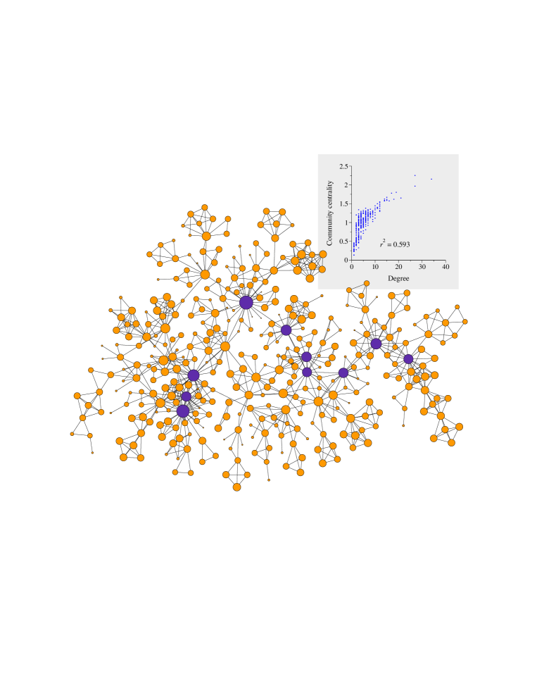
Figure 8: A network of coauthorships between 379 scientists whose research centers on the properties of networks of one kind or another. Vertex diameters indicate the community centrality and the ten vertices with highest centralities are highlighted. For those readers curious about the identities of the vertices, an annotated version of this figure, names and all, can be found at http://www.umich.edu/~mejn/centrality. Inset: a scatter plot of community centrality against vertex degrees. Like most centrality measures, this one is correlated with degree, though only moderately strongly.

Let us focus here on the vector magnitudes and define two centrality measures for vertices in a network equal to the magnitudes of the vertex vectors $\mathbf{x}_{i}$ and $\mathbf{y}_{i}$. (If we prefer, we could use $|\mathbf{x}_{i}|^{2}$ instead, which is slightly easier to calculate. If, as is sometimes the case with centrality measures, we only care about relative rankings of vertices, then the two are equivalent.) These centralities are now properties of the vertices alone and are independent of the way the network is divided into communities. We notice, however, that $|\mathbf{x}_{i}|$ and $|\mathbf{y}_{i}|$ are not independent since

$$|\mathbf{x}_{i}|^{2}-|\mathbf{y}_{i}|^{2} = \sum_{j=1}^{p}\bigl{(}\sqrt{\beta_{j}}\,U_{ij}\bigr{)}^{2}$$ (63)

$${}-\sum_{j=1}^{q}\bigl{(}\sqrt{-\beta_{n+1-j}}\,U_{i,{n+1-j}}\bigr{)}^{2}$$

$$= \sum_{j=1}^{n}U_{ij}\beta_{j}U_{ji}^{T}=B_{ii}.$$

Almost all networks considered in the literature are simple graphs, meaning, among other things, that they have no self-edges (edges that connect vertices to themselves) and hence $A_{ii}=0$ for all $i$. If the expected number of self-edges $P_{ii}$ is also zero (as seems sensible), then $B_{ii}=0$ and we have $|\mathbf{x}_{i}|=|\mathbf{y}_{i}|$ for all $i$. Thus there is actually only one centrality for simple graphs, not two.

In fact, the choice (23) for $P_{ij}$ that we and other authors have mostly used does allow self-edges (and is in this sense slightly unrealistic—see [56]), but $P_{ii}=k_{i}^{2}/2m$ is typically small for most vertices if $m$ is large (and indeed vanishes as $m\to\infty$ if degrees are bounded), and hence it is still true to a good approximation that $|\mathbf{x}_{i}|\simeq|\mathbf{y}_{i}|$ and there is only one centrality.

In other words, we come to the nontrivial conclusion that the vertices with the greatest capacity for making positive contributions to the modularity also have the greatest capacity for making negative contributions. The fundamental meaning of this centrality measure is thus that there are certain vertices that, as a consequence of their situation within the network, have the power to make substantial contributions, either positive or negative, to the overall modularity of the network. For this reason, we call this centrality measure community centrality. We define it to be equal to the vector magnitude $|\mathbf{x}_{i}|$.

An alternative way to view the community centrality is to consider how a vertex $i$ is situated among the other vertices in its immediate vicinity—its neighborhood in the network. If we were to artificially construct a community from the vertices of this neighborhood, then that community would presumably have a community vector $\mathbf{X}_{k}$ with direction close to $\mathbf{x}_{i}$, and hence the magnitude $|\mathbf{x}_{i}|$ would be a good measure of the actual strength with which vertex $i$ belongs the community. Thus vertices with high community centrality are ones that play a central role in their local neighborhood, regardless of where the official community boundaries may lie. Conversely, even when considered as the “center of its world” in this way, vertex $i$ can never play a central role in its neighborhood in this sense if $|\mathbf{x}_{i}|$ is small.

As an example, consider Fig. 8, which shows results for community centrality for a network of coauthorships between scientists, scientists in this case who are themselves publishing on the topic of networks. The network is similar to the one presented in Ref. [18] but is based on more recent data, including publications up until early 2006. The network has a total of 1589 scientists in it, from a broad variety of fields, but only the 379 falling in the largest connected component are shown in the figure. The diameters of the vertices in the figure are proportional to their community centrality (actually to $|\mathbf{x}_{i}|^{2}$—see above), and the ten vertices having the highest centralities are highlighted. A couple of remarks are worth making about the results. Without naming specific names, we observe that all of the highlighted authors are group leaders or senior researchers of groups working in this area. Thus community centrality appears to live up to its name in this admittedly anecdotal example: it highlights those vertices that are central in their local communities. Second, while the centrality is correlated with degree ($r^{2}=0.59$—see the inset figure), the two are not perfectly correlated and in particular some vertices have quite high centrality while having relatively low degree. This emphasizes the point that high centrality is an indicator of individuals who have more connections than expected within their neighborhood (and hence potentially make a large contribution to the modularity), rather than simply having a lot of connections.

IX Conclusions

In this paper, we have studied the problem of detecting community structure in networks. There is already a substantial body of theory supporting the view that community structure can be accurately quantified using the benefit function known as modularity and hence that communities can be detected by searching possible divisions of a network for ones that possess high modularity. Here we have demonstrated that the modularity can be succinctly expressed in terms of the eigenvalues and eigenvectors of a matrix we call the modularity matrix, which is a characteristic property of the network and is itself independent of any division of the network into communities. Using this expression we have derived a series of further results including several new and competitive algorithms for identifying communities, a method for detecting bipartite or $k$-partite structure in networks, and a new community centrality measure that identifies vertices that play a central role in the communities to which they belong.

We have demonstrated a variety of applications of our methods to real-world networks representing social, technological, and information networks. These, however, are intended only as illustrations of the potential of these methods. We hope that readers will feel encouraged to apply these or similar methods to other networks of scientific interest and we look forward to seeing the results.

- [1] M. E. J. Newman, The structure and function of complex networks. SIAM Review 45, 167–256 (2003).
- [2] S. Boccaletti, V. Latora, Y. Moreno, M. Chavez, and D.-U. Hwang, Complex networks: Structure and dynamics. Physics Reports 424, 175–308 (2006).
- [3] S. N. Dorogovtsev and J. F. F. Mendes, Evolution of Networks: From Biological Nets to the Internet and WWW. Oxford University Press, Oxford (2003).
- [4] M. E. J. Newman, A.-L. Barabási, and D. J. Watts, The Structure and Dynamics of Networks. Princeton University Press, Princeton (2006).
- [5] M. Girvan and M. E. J. Newman, Community structure in social and biological networks. Proc. Natl. Acad. Sci. USA 99, 7821–7826 (2002).
- [6] M. E. J. Newman, Detecting community structure in networks. Eur. Phys. J. B 38, 321–330 (2004).
- [7] P. Holme, M. Huss, and H. Jeong, Subnetwork hierarchies of biochemical pathways. Bioinformatics 19, 532–538 (2003).
- [8] R. Guimerà and L. A. N. Amaral, Functional cartography of complex metabolic networks. Nature 433, 895–900 (2005).
- [9] G. Palla, I. Derényi, I. Farkas, and T. Vicsek, Uncovering the overlapping community structure of complex networks in nature and society. Nature 435, 814–818 (2005).
- [10] G. W. Flake, S. R. Lawrence, C. L. Giles, and F. M. Coetzee, Self-organization and identification of Web communities. IEEE Computer 35, 66–71 (2002).
- [11] M. Huss and P. Holme, Currency and commodity metabolites: Their identification and relation to the modularity of metabolic networks. Preprint q-bio/0603038 (2006).
- [12] G. P. Garnett, J. P. Hughes, R. M. Anderson, B. P. Stoner, S. O. Aral, W. L. Whittington, H. H. Handsfield, and K. K. Holmes, Sexual mixing patterns of patients attending sexually transmitted diseases clinics. Sexually Transmitted Diseases 23, 248–257 (1996).
- [13] S. O. Aral, J. P. Hughes, B. Stoner, W. Whittington, H. H. Handsfield, R. M. Anderson, and K. K. Holmes, Sexual mixing patterns in the spread of gonococcal and chlamydial infections. American Journal of Public Health 89, 825–833 (1999).
- [14] S. Gupta, R. M. Anderson, and R. M. May, Networks of sexual contacts: Implications for the pattern of spread of HIV. AIDS 3, 807–817 (1989).
- [15] M. Granovetter, The strength of weak ties. Am. J. Sociol. 78, 1360–1380 (1973).
- [16] R. S. Burt, Positions in networks. Social Forces 55, 93–122 (1976).
- [17] L. C. Freeman, A set of measures of centrality based upon betweenness. Sociometry 40, 35–41 (1977).
- [18] M. E. J. Newman and M. Girvan, Finding and evaluating community structure in networks. Phys. Rev. E 69, 026113 (2004).
- [19] P. Pollner, G. Palla, and T. Vicsek, Preferential attachment of communities: The same principle, but a higher level. Europhys. Lett. 73, 478–484 (2006).
- [20] H. Zhou, Distance, dissimilarity index, and network community structure. Phys. Rev. E 67, 061901 (2003).
- [21] A. E. Krause, K. A. Frank, D. M. Mason, R. E. Ulanowicz, and W. W. Taylor, Compartments revealed in food-web structure. Nature 426, 282–285 (2003).
- [22] F. Wu and B. A. Huberman, Finding communities in linear time: A physics approach. Eur. Phys. J. B 38, 331–338 (2004).
- [23] F. Radicchi, C. Castellano, F. Cecconi, V. Loreto, and D. Parisi, Defining and identifying communities in networks. Proc. Natl. Acad. Sci. USA 101, 2658–2663 (2004).
- [24] M. E. J. Newman, Fast algorithm for detecting community structure in networks. Phys. Rev. E 69, 066133 (2004).
- [25] A. Capocci, V. D. P. Servedio, G. Caldarelli, and F. Colaiori, Detecting communities in large networks. In S. Leonardi (ed.), Proceedings of the 3rd Workshop on Algorithms and Models for the Web Graph, number 3243 in Lecture Notes in Computer Science, Springer, Berlin (2004).
- [26] S. Fortunato, V. Latora, and M. Marchiori, A method to find community structures based on information centrality. Phys. Rev. E 70, 056104 (2004).
- [27] J. Reichardt and S. Bornholdt, Detecting fuzzy community structures in complex networks with a Potts model. Phys. Rev. Lett. 93, 218701 (2004).
- [28] L. Donetti and M. A. Muñoz, Detecting network communities: A new systematic and efficient algorithm. J. Stat. Mech. p. P10012 (2004).
- [29] H. Zhou and R. Lipowsky, Network brownian motion: A new method to measure vertex-vertex proximity and to identify communities and subcommunities. In Lecture Notes in Computer Science, volume 3038, pp. 1062–1069, Springer, New York (2004).
- [30] A. Clauset, Finding local community structure in networks. Phys. Rev. E 72, 026132 (2005).
- [31] P. Pons and M. Latapy, Computing communities in large networks using random walks. In Proceedings of the 20th International Symposium on Computer and Information Sciences, volume 3733 of Lecture Notes in Computer Science, pp. 284–293, Springer, New York (2005).
- [32] M. E. J. Newman, Modularity and community structure in networks. Preprint physics/0602124 (2006).
- [33] L. Danon, A. Diaz-Guilera, and A. Arenas, Effect of size heterogeneity on community identification in complex networks. Preprint physics/0601144 (2006).
- [34] J. Reichardt and S. Bornholdt, Statistical mechanics of community detection. Preprint cond-mat/0603718 (2006).
- [35] M. B. Hastings, Community detection as an inference problem. Preprint cond-mat/0604429 (2006).
- [36] L. Danon, J. Duch, A. Diaz-Guilera, and A. Arenas, Comparing community structure identification. J. Stat. Mech. p. P09008 (2005).
- [37] M. Gustafsson, A. Lombardi, and M. Hornquist, Comparison and validation of community structures in complex networks. Preprint physics/0601057 (2006).
- [38] A. Clauset, M. E. J. Newman, and C. Moore, Finding community structure in very large networks. Phys. Rev. E 70, 066111 (2004).
- [39] R. Guimerà, M. Sales-Pardo, and L. A. N. Amaral, Modularity from fluctuations in random graphs and complex networks. Phys. Rev. E 70, 025101 (2004).
- [40] J. Duch and A. Arenas, Community detection in complex networks using extremal optimization. Phys. Rev. E 72, 027104 (2005).
- [41] M. Fiedler, Algebraic connectivity of graphs. Czech. Math. J. 23, 298–305 (1973).
- [42] A. Pothen, H. Simon, and K.-P. Liou, Partitioning sparse matrices with eigenvectors of graphs. SIAM J. Matrix Anal. Appl. 11, 430–452 (1990).
- [43] P.-O. Fjällström, Algorithms for graph partitioning: A survey. Linköping Electronic Articles in Computer and Information Science 3(10) (1998).
- [44] O. Goldschmidt and D. S. Hochbaum, Polynomial algorithm for the -cut problem. In Proceedings of the 29th Annual IEEE Symposium on the Foundations of Computer Science, pp. 444–451, Institute of Electrical and Electronics Engineers, New York (1988).
- [45] F. R. K. Chung, Spectral Graph Theory. Number 92 in CBMS Regional Conference Series in Mathematics, American Mathematical Society, Providence, RI (1997).
- [46] B. Bollobás, Modern Graph Theory. Springer, New York (1998).
- [47] M. Barahona and L. M. Pecora, Synchronization in small-world systems. Phys. Rev. Lett. 89, 054101 (2002).
- [48] T. Nishikawa, A. E. Motter, Y.-C. Lai, and F. C. Hoppensteadt, Heterogeneity in oscillator networks: Are smaller worlds easier to synchronize? Phys. Rev. Lett. 91, 014101 (2003).
- [49] M. Bern, D. Eppstein, and J. Gilbert, Provably good mesh generation. In Proceedings of the 31st Annual IEEE Symposium on the Foundations of Computer Science, pp. 231–241, Institute of Electrical and Electronics Engineers, New York (1990).
- [50] Y.-C. Wei and C.-K. Cheng, Toward efficient hierarchical designs by ratio cut partitioning. In Proceedings of the IEEE International Conference on Computer Aided Design, pp. 298–301, Institute of Electrical and Electronics Engineers, New York (1989).
- [51] L. Hagen and A. B. Kahng, New spectral methods for ratio cut partitioning and clustering. IEEE Transations on Computer-Aided Design 11, 1074–1085 (1992).
- [52] P. K. Chan, M. D. F. Schlag, and J. Y. Zien, Spectral -way ratio-cut partitioning and clustering. In Proceedings of the 30th International Conference on Design Automation, pp. 749–754, Association of Computing Machinery, New York (1993).
- [53] M. E. J. Newman, Mixing patterns in networks. Phys. Rev. E 67, 026126 (2003).
- [54] M. E. J. Newman, Analysis of weighted networks. Phys. Rev. E 70, 056131 (2004).
- [55] S. White and P. Smyth, A spectral clustering approach to finding communities in graphs. In H. Kargupta, J. Srivastava, C. Kamath, and A. Goodman (eds.), Proceedings of the 5th SIAM International Conference on Data Mining, Society for Industrial and Applied Mathematics, Philadelphia (2005).
- [56] C. P. Massen and J. P. K. Doye, Identifying “communities” within energy landscapes. Phys. Rev. E 71, 046101 (2005).
- [57] S. H. Strogatz, Exploring complex networks. Nature 410, 268–276 (2001).
- [58] S. N. Dorogovtsev and J. F. F. Mendes, Evolution of networks. Advances in Physics 51, 1079–1187 (2002).
- [59] D. J. Watts and S. H. Strogatz, Collective dynamics of ‘small-world’ networks. Nature 393, 440–442 (1998).
- [60] A.-L. Barabási and R. Albert, Emergence of scaling in random networks. Science 286, 509–512 (1999).
- [61] L. A. N. Amaral, A. Scala, M. Barthélémy, and H. E. Stanley, Classes of small-world networks. Proc. Natl. Acad. Sci. USA 97, 11149–11152 (2000).
- [62] F. Chung and L. Lu, Connected components in random graphs with given degree sequences. Annals of Combinatorics 6, 125–145 (2002).
- [63] T. Łuczak, Sparse random graphs with a given degree sequence. In A. M. Frieze and T. Łuczak (eds.), Proceedings of the Symposium on Random Graphs, Poznań 1989, pp. 165–182, John Wiley, New York (1992).
- [64] M. Molloy and B. Reed, A critical point for random graphs with a given degree sequence. Random Structures and Algorithms 6, 161–179 (1995).
- [65] M. E. J. Newman, S. H. Strogatz, and D. J. Watts, Random graphs with arbitrary degree distributions and their applications. Phys. Rev. E 64, 026118 (2001).
- [66] R. Pastor-Satorras, A. Vázquez, and A. Vespignani, Dynamical and correlation properties of the Internet. Phys. Rev. Lett. 87, 258701 (2001).
- [67] M. E. J. Newman, Assortative mixing in networks. Phys. Rev. Lett. 89, 208701 (2002).
- [68] D. Lusseau, K. Schneider, O. J. Boisseau, P. Haase, E. Slooten, and S. M. Dawson, The bottlenose dolphin community of Doubtful Sound features a large proportion of long-lasting associations. Can geographic isolation explain this unique trait? Behavioral Ecology and Sociobiology 54, 396–405 (2003).
- [69] C. J. Alpert and S.-Z. Yao, Spectral partitioning: The more eigenvectors, the better. In B. T. Preas, P. G. Karger, B. S. Nobandegani, and M. Pedram (eds.), Proceedings of the 32nd International Conference on Design Automation, pp. 195–200, Association of Computing Machinery, New York, NY (1995).
- [70] C. D. Meyer, Matrix Analysis and Applied Linear Algebra. Society for Industrial and Applied Mathematics, Philadelphia (2000).
- [71] B. W. Kernighan and S. Lin, An efficient heuristic procedure for partitioning graphs. Bell System Technical Journal 49, 291–307 (1970).
- [72] J. M. Kleinberg, Authoritative sources in a hyperlinked environment. J. ACM 46, 604–632 (1999).
- [73] P. Holme, F. Liljeros, C. R. Edling, and B. J. Kim, Network bipartivity. Phys. Rev. E 68, 056107 (2003).
- [74] E. Estrada and J. A. Rodríguez-Velázquez, Spectral measures of bipartivity in complex networks. Phys. Rev. E 72, 046105 (2005).