Space Charges Can Significantly Affect the Dynamics of Accelerator Maps

Abstract

Space charge effects can be very important for the dynamics of intense particle beams, as they repeatedly pass through nonlinear focusing elements, aiming to maximize the beam’s luminosity properties in the storage rings of a high energy accelerator. In the case of hadron beams, whose charge distribution can be considered as “frozen” within a cylindrical core of small radius compared to the beam’s dynamical aperture, analytical formulas have been recently derived BenTurc for the contribution of space charges within first order Hamiltonian perturbation theory. These formulas involve distribution functions which, in general, do not lead to expressions that can be evaluated in closed form. In this paper, we apply this theory to an example of a charge distribution, whose effect on the dynamics can be derived explicitly and in closed form, both in the case of 2–dimensional as well as 4–dimensional mapping models of hadron beams. We find that, even for very small values of the “perveance” (strength of the space charge effect) the long term stability of the dynamics changes considerably. In the flat beam case, the outer invariant “tori” surrounding the origin disappear, decreasing the size of the beam’s dynamical aperture, while beyond a certain threshold the beam is almost entirely lost. Analogous results in mapping models of beams with 2-dimensional cross section demonstrate that in that case also, even for weak tune depressions, orbital diffusion is enhanced and many particles whose motion was bounded now escape to infinity, indicating that space charges can impose significant limitations on the beam’s luminosity.

I Introduction

One of the fundamental problems concerning the dynamics of particle beams in the storage rings of high energy accelerators is the determination of the beam’s dynamical aperture, i.e. the maximal domain containing the particles closest to their ideal circular path and for the longest possible time. For example, “flat” hadron beams (experiencing largely horizontal betatron oscillations) can be described by 2–dimensional (2D) area–preserving maps, where the existence of invariant curves around the ideal stable path at the origin, guarantees the stability of the beam’s dynamics for infinitely long times BTTS94 ; GT96 . The reason for this is that the chaotic motion between these invariant curves is always bounded and the particles never escape to infinity. Other important phenomena that arise in this context is the presence of a major resonance in the form of a chain of islands through which the beam may be collected, or the existence of an outer invariant curve surrounding these islands, which serves as a boundary of the motion and thus allows an estimate of the beam’s dynamical aperture.

On the other hand, hadron beams with a 2 - dimensional cross section require the use of $4$–dimensional (4D) symplectic mappings for the study of their dynamics BT91 ; BK94 ; VBK96 ; VIB97 ; BS05 . In fact, if longitudinal (or synchrotron) oscillations also need to be included the mappings become 6–dimensional. In such cases, the problems of particle loss are severe, as chaotic regions around different resonances are connected, providing a network of paths through which particles can move away from the origin, and eventually escape from the beam after sufficiently long times.

In this Letter, we add to these issues the presence of space charges within a core radius $r_{c}$, which is small compared to the beam’s dynamical aperture. In other words, we will assume that our proton (or antiproton) beam is intense enough so that the effect of a charge distribution concentrated within this core radius cannot be neglected. Furthermore, we will consider this distribution as cylindrically symmetric and “frozen” (i.e. time independent, so that it may be self consistent with the linear lattice) and study the dynamics of a hadron beam as it passes repeatedly through nonlinear magnetic focusing elements of the FODO cell type. This system has been studied extensively in the absence of space charge effects in BTTS94 ; GT96 ; BT91 ; BK94 ; VBK96 ; VIB97 ; BS05 and the question we raise now is whether its dynamics can be seriously affected if space charges are also taken into consideration.

Space charge presents a fundamental limitation to high intensity circular accelerators. Its effects are especially important in the latest designs of high-intensity proton rings, which require beam losses much smaller than presently achieved in existing facilities. It is therefore necessary to estimate the major space charge effects which could lead to emittance growth and associated beam loss Fedotov . The interplay between nonlinear effects, typical of single-particle dynamics, and space charge, typical of multi-particle dynamics induced by the Coulomb interaction, represents a difficult challenge. To understand better these phenomena, an intense experimental campaign was launched at the CERN Proton Synchrotron Franchetti_2003 . It is very important, therefore, to develop analytical techniques which could be utilized in order to study and localize the associated web of resonances (see e.g. PAC2001 ) to obtain an analytical estimation of the dynamic aperture, as suggested e.g. in Benedetti .

In a recent paper, Benedetti and Turchetti BenTurc used first order canonical perturbation theory to obtain analytical expressions for the jump in the position and momenta due to the multipolar kicks in such maps, showing that the space charges effectively modulate the tune at every passage of the particle through a nonlinear element of the lattice. In particular, they derived the new position and momentum coordinates after the $n$th passage through a FODO cell in the thin lens approximation, as the iterates of the 2D map

$$\left(\begin{array}[]{c}X_{n+1}\\ P_{n+1}\end{array}\right)=\left(\begin{array}[]{cc}\cos\Omega(J)&-\sin\Omega(J)\\ \sin\Omega(J)&\ \cos\Omega(J)\\ \end{array}\right)\times\left(\begin{array}[]{c}X_{n}\\ P_{n}+X_{n}^{k-1}\\ \end{array}\right),\ \ n=0,1,2,...,$$ (1)

where

$$J=\frac{P_{n}^{2}+X_{n}^{2}}{2},$$ (2)

for $k=3$, i.e. in the case of sextupole nonlinearities and

$$\Omega(J)=\omega+\frac{\omega_{0}^{2}-\omega^{2}}{2\omega}\left(1-\frac{R_{c}^{2}}{J}\frac{1}{2\pi}\int_{0}^{2\pi}g_{1}\left(\frac{2J\cos^{2}\theta}{R_{c}^{2}}\right)d\theta\right).$$ (3)

The variables $P$, $X$ and the parameters entering in the above expressions are related to the corresponding ones of the original Hamiltonian

$$H=\frac{p^{2}}{2}+\omega_{0}^{2}\frac{x^{2}}{2}-\frac{x^{3}}{3}\sum_{l=1,2,..}\delta(s-l)-\frac{\xi}{2}g_{2}\left(\frac{x^{2}}{r_{c}^{2}}\right),$$ (4)

by the formulas

$$P=p/\omega^{2}\ ,\ X=x/\omega\ ,\ \ R_{c}=r_{c}\omega^{-3/2}\ ,\ \ \omega^{2}=\omega_{0}^{2}-\frac{\xi}{r_{c}^{2}},$$ (5)

where $\omega$ is the depressed phase advance at the center of the charge distribution, $p=dx/ds$, $s$ is the coordinate along the ideal circular orbit, $g_{2}(t)$ is given by

$$g_{2}(t)=\int_{0}^{t}u^{-1}g_{1}(u)du\ ,\ g_{1}(t)=\int_{0}^{t}g(u)du\ ,\ g\left(\frac{r^{2}}{r_{c}^{2}}\right)=\pi r_{c}^{2}\rho(r)$$ (6)

$\rho(r)$ satisfies $\int_{0}^{\infty}\pi\rho(r)dr^{2}=1$, $\pi r_{c}^{2}\rho(0)=1$ and $Q\rho(r)$ represents the radial charge density. Note that if $m$, $q$, and $v_{0}$ denote the mass, charge and velocity of our non-relativistic particles, the “perveance” parameter $\xi=2qQ/mv_{0}^{2}$ determines the tune depression in (5), which must be small for the above analysis to be valid BenTurc .

The stage is now set for the investigation of space charge effects on the dynamics. However, the space advances $\Omega(J)$ needed in (1) at every iteration depend on integrals of the distribution function $g(u)$ that may not be available analytically. To overcome this difficulty, we choose in section II a particular form of $g(u)$ for which these integrals can be explicitly carried out not only for 2D maps of the “flat” beam case, but also for 4D maps describing vertical as well as horizontal deflections of the beam’s particles.

Thus, in section III we perform numerical experiments to examine the influence of space charges on the dynamics and find indeed that even for small perveance values the long term stability of the beam is significantly affected. In particular, as $\xi$ grows (or the tune depression $\omega/\omega_{0}$ decreases from 1), perturbations of 2D as well as 4D maps show that the outer invariant “surfaces” surrounding the ideal circular path at the origin disappear and the beam’s dynamical aperture is seriously limited. Only the major unperturbed stable resonances survive, with their “boundaries” clearly diminished by the presence of new resonances due to space charge effects. In our 2D mapping model, a threshold value of $\xi$ (or $\omega/\omega_{0}$) was found, beyond which the beam is practically destroyed. The paper ends by describing our concluding remarks and work in progress in section IV.

Space charge effects on beam stability became a relevant topic during the years when construction of medium-low energy high currents accelerators, such as SNS and the design of the FAIR rings at GSI were started Jeon ; PAC2001 ; Franchetti_2005 (see also many articles in the SNS Accelerator Physics Proceedings of the last few years). The role of collective effects and resonances has attracted considerable attention, since they can cause significant beam quality deterioration and losses Hofmann . Another relevant issue is the coupling with the longitudinal motion which modulates the transverse tune and induces losses by resonance crossing as shown by recent experiments Franchetti_2003 .

High intensity rings, where the bunches can circulate over one million turns, require a careful analysis of the long term stability of the beam. Since the commonly used codes require large CPU times and exhibit an emittance growth due to numerical noise, they are not suited for long term dynamic aperture studies and the use of faster methods is necessary Franchetti_2005 . The method proposed in BenTurc allows us to introduce space charge effects in one single evaluation of the map, when a thin sextupole or octupole is present, just as one does in the absence of space charge, and is thus especially well suited for dynamical aperture calculations.

II Exact Results for a Specific Charge Distribution

II.1 The One - dimensional Beam

Let us choose for our space charge distribution function in the 1–dimensional case the form

$$g\left(\frac{X^{2}}{R_{c}^{2}}\right)=\frac{1}{(X^{2}/R_{c}^{2}+1)^{2}}\,\,.$$ (7)

The generalization to 2 dimensions is evident by replacing $X^{2}$ by $X^{2}+Y^{2}$ in (7). Observe that this function satisfies the requirements that $g(0)=1$, $g_{1}(t)\propto t$ as $t\rightarrow 0$ and $g_{1}(t)\rightarrow 1$ as $t\rightarrow 0$, (using (6)), as expected from the theory BenTurc .

Evaluating now by elementary manipulations the integral in (3), using (7) and (6), we find that it is given by the closed form expression

$$\int_{0}^{2\pi}g_{1}\left(\frac{2J\cos^{2}\theta}{R_{c}^{2}}\right)d\theta=2\pi-\frac{2\pi}{(\frac{2J}{R_{c}^{2}}+1)^{1/2}}\,\,.$$ (8)

Thus, the phase advance at every iteration becomes

$$\Omega(J)=\omega+\frac{\omega_{0}^{2}-\omega^{2}}{2\omega}\left(1-\frac{R_{c}^{2}}{J}+\frac{R_{c}^{2}}{J(\frac{2J}{R_{c}^{2}}+1)^{1/2}}\right),$$ (9)

where $J$ is given by (2). Note that, in the limit $J\rightarrow 0$, eq. (9) implies that $\Omega\rightarrow\omega$ as expected. In fact, expanding the square root in that limit we find

$$\Omega(J)=\omega+\frac{\omega_{0}^{2}-\omega^{2}}{2\omega}\left(\frac{3}{2}\frac{J}{R_{c}^{2}}-\frac{5}{2}\frac{J^{2}}{R_{c}^{4}}+...\right),$$ (10)

from which we can estimate the deviation of $\Omega$ from the depressed tune $\omega$ near the origin. In section III below we pick an $\omega_{0}$ such that for $\xi=0$ we have a major resonance and a relatively large dynamical aperture in the $X_{n},P_{n}$ plane, select $r_{c}$ small compared with this aperture and vary $\xi$ to study the space charge effect on the dynamics.

II.2 The Two - dimensional Beam

Let us now observe that in two space dimensions the original Hamiltonian of the system, (4), becomes

$$H=\frac{p_{1}^{2}}{2}+\omega_{01}^{2}\frac{x^{2}}{2}+\frac{p_{2}^{2}}{2}+\omega_{02}^{2}\frac{y^{2}}{2}+\left(-\frac{x^{3}}{3}+xy^{2}\right)\sum_{l=1,2,..}\delta(s-l)-\frac{\xi}{2}g_{2}\left(\frac{x^{2}+y^{2}}{r_{c}^{2}}\right),$$ (11)

where sextupole nonlinearities involve, of course, both $x$ and $y$ variables. Since there are now two tune depressions

$$\omega_{1}=\left(\omega_{01}^{2}-\frac{\xi}{r_{c}^{2}}\right)^{1/2}\ \ ,\ \ \omega_{2}=\left(\omega_{02}^{2}-\frac{\xi}{r_{c}^{2}}\right)^{1/2},$$ (12)

after transforming to new variables $X=x\omega_{1}^{1/2}$, $P_{1}=p_{1}\omega_{1}^{-1/2}$ and $Y=y\omega_{2}^{1/2}$, $P_{2}=p_{2}\omega_{2}^{-1/2}$ defined by

$$X=(2J_{1})^{1/2}\cos\theta_{1}\ ,\ P_{1}=-(2J_{1})^{1/2}\sin\theta_{1}\ ,\ Y=(2J_{2})^{1/2}\cos\theta_{2}\ ,\ P_{2}=-(2J_{2})^{1/2}\sin\theta_{2},$$ (13)

differentiating the Hamiltonian with respect to $J_{1}$ and $J_{2}$ and integrating over $\theta_{1}$ and $\theta_{2}$, we find the two tune depressions

$$\Omega_{1}=\omega_{1}+\frac{\omega_{01}^{2}-\omega_{1}^{2}}{2\omega_{1}}\left(1-\frac{1}{(2\pi)^{2}}\int_{0}^{2\pi}\int_{0}^{2\pi}\frac{2\cos^{2}\theta_{1}}{A+1}d\theta_{1}d\theta_{2}\right)$$ (14)

and $\Omega_{2}$, with 1 replaced by 2 in (14), while A is defined by

$$A=\frac{2J_{1}\cos^{2}\theta_{1}}{r_{1}^{2}}+\frac{2J_{2}\cos^{2}\theta_{2}}{r_{2}^{2}}\ ,\$$ (15)

where $r_{1}=r_{c}\omega_{1}^{1/2}$, $r_{2}=r_{c}\omega_{2}^{1/2}$.

Observe that we have used for the $g_{1}$ function under the integral sign (see (3)), the expression $g_{1}(A)=A/(1+A)$, derived from our simple choice of the distribution function (7) using (6).

The above $\Omega_{1}$ and $\Omega_{2}$ are to be used in the iterations of the 4D mapping:

$$\left(\begin{array}[]{c}X(n+1)\\ P_{1}(n+1)\\ Y(n+1)\\ P_{2}(n+1)\end{array}\right) = \left(\begin{array}[]{cccc}\cos\Omega_{1}&-\sin\Omega_{1}&0&0\\ \sin\Omega_{1}&\cos\Omega_{1}&0&0\\ 0&0&\cos\Omega_{2}&-\sin\Omega_{2}\\ 0&0&\sin\Omega_{2}&\cos\Omega_{2}\end{array}\right)$$ (24)

$$\times \left(\begin{array}[]{c}X(n)\\ P_{1}(n)+X^{2}(n)-Y^{2}(n)\\ Y(n)\\ P_{2}(n)-2X(n)Y(n)\end{array}\right),$$ (29)

whose dynamics has already been studied extensively in BT91 ; BK94 ; VBK96 ; VIB97 ; BS05 in the absence of space charge effects, i.e for $\omega_{1}=\omega_{01}$ and $\omega_{2}=\omega_{02}$. In these papers, it was observed that for the tune values $q_{x}=0.61903$, and $q_{y}=0.4152$, in

$$\omega_{01}=2\pi q_{x},\,\,\omega_{02}=2\pi q_{y},$$ (30)

a large dynamical aperture is achieved, with interesting chains of resonant “tori” surrounding the origin. In section III we will study what happens to these structures when $\xi>0$ (i.e $\omega_{1}<\omega_{01}$, $\omega_{2}<\omega_{02}$) and space charge effects are taken into account. Before doing this, however, it is necessary to describe how the integrals in (14) are to be evaluated: Let us first perform the integration over $\theta_{2}$, writing

$$K_{1}=\int_{0}^{2\pi}\int_{0}^{2\pi}\frac{2\cos^{2}\theta_{1}}{A+1}d\theta_{1}d\theta_{2}=2\int_{0}^{2\pi}d\theta_{1}\cos^{2}\theta_{1}I(\theta_{1}),$$ (31)

where

$$I(\theta_{1})=\int_{0}^{2\pi}\frac{d\theta_{2}}{2A_{1}\cos^{2}\theta_{2}+B_{1}}\ ,\ A_{1}=\frac{J_{2}}{r_{2}^{2}}\ ,\ B_{1}=1+\frac{2J_{1}\cos^{2}\theta_{1}}{r_{1}^{2}}\,\,.$$ (32)

The integral (32) can be evaluated as before with elementary functions to yield

$$I(\theta_{1})=\frac{2\pi}{[B_{1}(B_{1}+2A_{1})]^{1/2}}=2\pi\left[\left(1+\frac{2J_{1}\cos^{2}\theta_{1}}{r_{1}^{2}}\right)\left(1+\frac{2J_{1}\cos^{2}\theta_{1}}{r_{1}^{2}}+\frac{2J_{2}}{r_{2}^{2}}\right)\right]^{-1/2}\,\,.$$ (33)

Inserting now expression (33) into the integral (31), changing integration variable to $\phi=2\theta_{1}$, we easily arrive, after some simple manipulations, to the expression

$$K_{1}=\frac{2\pi r_{1}^{2}}{J_{1}}\int_{0}^{2\pi}d\phi\frac{cos\phi+1}{\left[(cos\phi+C_{1})(cos\phi+D_{1})\right)]^{1/2}}\,\,,$$ (34)

where

$$C_{1}=1+\frac{r_{1}^{2}}{J_{1}}\ ,\ D_{1}=1+\frac{r_{1}^{2}}{J_{1}}\left(1+\frac{2J_{2}}{r_{2}^{2}}\right).$$ (35)

We finally make the substitution $u=\tan(\phi/2)$ and rewrite the above integral in the form

$$K_{1}=\frac{16\pi r_{1}^{2}}{J_{1}}\int_{0}^{\infty}\frac{du}{(u^{2}+1)\left\{\left[(C_{1}-1)u^{2}+1+C_{1}\right]\left[(D_{1}-1)u^{2}+1+D_{1}\right]\right\}^{1/2}}\,\,.$$ (36)

This is clearly not an elementary integral. Notice, however, that all terms in the denominator of (36) are positive and as $u\rightarrow\infty$ the integrand vanishes as $u^{-4}$. It is, therefore, expected to converge very rapidly and may be computed, at every iteration of the map, using standard routines. For practical purposes, however, in section III below, we prefer to compute instead its equivalent form (34). Of course, as explained above, a similar integral, $K_{2}$, also needs to be computed (with $1\rightarrow 2$ in (31), (34) and (35)), whence $\Omega_{1}$ and $\Omega_{2}$ are found and the next iteration of the 4D map (29) can be evaluated.

III Numerical Results

Let us now turn to some practical applications of the above theory to specific problems concerning the stability of hadron beams passing through FODO cell magnetic focusing elements and experiencing sextupole nonlinearities, as described in BTTS94 ; GT96 ; BT91 . First, we shall consider the flat beam case (1), for the specific tune value $q_{x}=0.21$ corresponding to frequency $\omega_{0}=2\pi q_{x}=1.32$, exhibiting, in the absence of space charge perturbations, the phase space picture shown in Figure 1(a) below. As we see in this figure, the region of bounded particle motion extends to a radius of about 0.54 units from the origin. There are also 5 islands of a major resonance surrounded by invariant curves (or 1D “tori”), whose outermost boundary delimits the so - called dynamical aperture of the beam. Outside that domain there are chains of smaller islands (representing higher order resonances) and chaotic regions through which particles eventually escape to infinity. This escape occurs, of course, at different speeds due to the well - known phenomenon of “stickiness”, depending on how close the orbits are to the invariant curves surrounding the islands.

Let us now consider a space charge distribution of the form (7) with a “frozen core” of radius $r_{c}=0.1$, which is small compared with the radius of the beam’s dynamical aperture. Our purpose is to vary the value of the preveance $\xi>0$, cf. (4), starting from $\xi=0$, to estimate the effects of space charge on the dynamics.

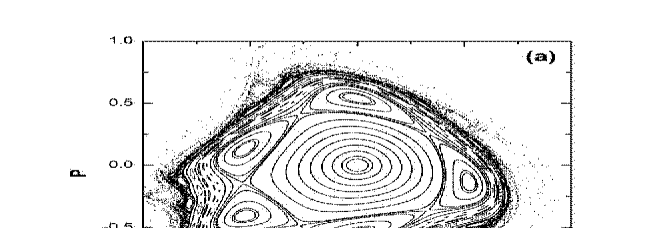
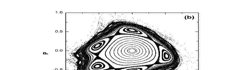
Figure 1: (a) The phase space picture of a flat beam, resulting from the iterations of the map (1), with tune $q_{x}=0.21$ and frequency $\omega_{0}=1.32$, in the absence of space charges. (b) The same picture with $\xi=0.001$ (or $\omega/\omega_{0}\simeq 0.9426$) in the Hamiltonian (4). Notice the dissolution of the outer invariant curves and the disappearance of many of the smaller islands of (a) away from the origin, leading to a significant decrease of the beam’s dynamical aperture. Each initial condition is followed for $N=10^{4}$ iterations.

Setting $\xi=0.001$ ($\omega/\omega_{0}\simeq 0.97$), for example, which is quite small compared with $r_{c}^{2}=0.01$, we observe in Figure 1(b) that the picture has significantly changed. In particular, the 3-dimensional character of the dynamics (due to the variation of the space advance $\Omega(J)$) has turned the invariant curves into “surfaces” and has led to the dissolution of the outer ones surrounding the five major islands. Furthermore, most of the chains of smaller islands of Figure 1(a) have disappeared due to the new resonances caused by the presence of space charges. To see how all this affects the dynamical aperture of the beam as a function of the tune depression $\omega/\omega_{0}$ we now perform the following experiment:

Forming a grid of initial conditions of step size $\Delta x=\Delta p=0.01$ within a square $[-1,1]\times[-1,1]$ about the origin ($X_{n}=P_{n}=0$), we use (1) to iterate for different $\xi>0$ (or $\omega/\omega_{0}<1$) all points falling within circular rings of width $\Delta r=0.01$ for $N=10^{5}$ and $N=10^{6}$ iterations and plot in Figure 2 the last $r=(X_{n}^{2}+P_{n}^{2})^{1/2}=r_{esc}$ value, at which at least one orbit was found to escape from the next outer ring. The results demonstrate that already at $\xi=0.001$ ($\omega/\omega_{0}\simeq 0.97$) our estimate of the dynamical aperture $r_{esc}$ has fallen from $0.54$ to about $0.43$. In fact, it remains close to that value (rising somewhat to about $0.5$) until $\xi\simeq.006$ ($\omega/\omega_{0}\simeq 0.81$), where it experiences a sudden drop to $r_{esc}\simeq 0.03$, and the beam is effectively destroyed. Of course, once one orbit escapes most of them quickly follow within the next one or two circular rings. Note also that increasing the number of iterations from $N=10^{5}$ to $N=10^{6}$ does not appreciably change the results, until the sudden drop occurs.

Figure 2: Plot of dynamical aperture “radius” $r_{esc}$ estimates of the flat beam case, resulting from the iterations of the map (1), with frequency $\omega_{0}=1.32$, in the presence of space charges, i.e for increasing values of $\xi$ in (4). Note the quick decrease of the aperture value by about $20$ percent, which remains nearly the same until $\xi\simeq 0.006$ ($\omega/\omega_{0}\simeq 0.81$), when a sudden drop occurs, probably due to the appearance of a major new resonance.

This dramatic change at $\omega/\omega_{0}\simeq 0.81$ is most probably due to the presence of a major new resonance caused by the space charge perturbation. It may be an important effect, however, since it occurs at a $\xi$ value which is still smaller than the $r_{c}^{2}=0.01$ radius of the charge core. Of course, long before this happens, already at $\xi\simeq 0.0002$ (or $\omega/\omega_{0}\simeq 0.994$), the effective aperture of the beam has been significantly reduced by about 20 percent from its value at $\xi=0$.

Finally, let us turn to the case of the 4D map (29), describing the more realistic case of a beam whose particles experience horizontal as well as vertical displacements from the ideal path, see (11). For comparison purposes, we choose the same parameter values as in our earlier papers BK94 ; VBK96 ; VIB97 ; BS05 , i.e horizontal and vertical tunes $q_{x}=0.61903$, $q_{y}=0.4152$ respectively, yielding the unperturbed frequencies (30) used in the mapping equations. In Figure 3(a), we iterate many initial conditions $X(0),P_{1}(0),Y(0),P_{2}(0)$ around the origin and plot on a $X(n),P_{1}(n)$ projection a picture of the dynamics, for $|Y(n)|\leq 0.04$, in the absence of space charges, i.e. with $\omega_{i}=\omega_{0i}$, $i=1,2$.

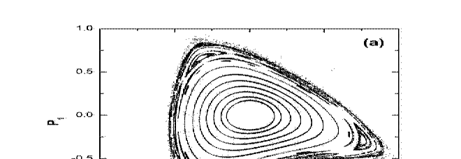
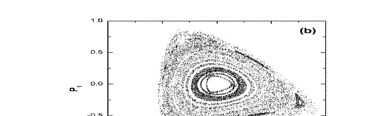
Figure 3: (a) An $X,P_{1}$ projection of a beam with $x$ and $y$ deflections, resulting from the iterations of the map (29), with tunes $q_{x}=0.61903,q_{y}=0.4152$, in the absence of space charges. Note the presence of a large region of invariant 2D “tori” about the origin and the 6 “islands” of a stable resonance, shown here in a cut of the 4D space, with $|Y(n)|\leq 0.04$. (b) The same picture with $\xi=0.0002$ in Hamiltonian (11) (or $\omega_{1}/\omega_{01}\simeq 0.9993,\omega_{2}/\omega_{02}\simeq 0.9985$). Each initial condition is followed for $N=10^{4}$ iterations. Notice the dissolution of outer invariant curves surrounding the origin and the disappearance of the chain of islands of (a), leading to a significant decrease of the beam’s dynamical aperture.

Note the region of invariant tori and a chain of 6 “islands” corresponding to a stable resonance. Strictly speaking, the motion between these tori need not be bounded as 2D surfaces do not separate 4D space and Arno’ld diffusion phenomena Licht-Lieb could in principle carry orbits far away from the origin. However, as has been explicitly shown for this model in BK94 ; VBK96 ; VIB97 , such phenomena are extremely slow and hence a domain with radius of the order of 0.5 can be effectively considered as the dynamical aperture of the beam. Repeating this experiment in the presence of space charges, i.e. with $\xi=0.0002$ (or $\omega_{1}/\omega_{01}\simeq 0.9993,\omega_{2}/\omega_{02}\simeq 0.9985$) in (11), we observe in Figure 3(b) that the outer invariant curves (together with the islands) have been destroyed and the dynamical aperture of the beam has been significantly reduced.

Studying this reduction as a function of $\xi$, we proceed to choose initial conditions from a grid of step size 0.05, extending from -0.65 to 0.65 in all 4 directions about the origin, represented by $X(0),P_{1}(0),Y(0),P_{2}(0)$. Iterating the resulting orbits from points within spherical shells of width $\Delta r=0.01$, we plot in Figure 4, for each $\xi$, the $r_{esc}$ value of the inner radius of the shell from which at least one orbit escapes to infinity. Our results demonstrate that the beam’s dynamical aperture steadily decreases as $\xi$ grows. At $\xi=0.006$ (or $\omega_{1}/\omega_{01}\simeq 0.98,\omega_{2}/\omega_{02}\simeq 0.955$) its radius has fallen by more than 50 percent from its original value, while at higher perveance values the approximation $\xi<<r_{c}^{2}$ no longer applies. In fact, it is worth noting that the size of the dynamical aperture falls drastically even for small values of $\xi$, as our calculations with $N=10^{5}$ iterations show. For example even at $\xi=0.0002$ (or $\omega_{1}/\omega_{01}\simeq 0.9993,\omega_{2}/\omega_{02}\simeq 0.9985$) our estimate of the dynamical aperture has dropped from 0.54 to 0.37.

Figure 4: Plot of dynamical aperture estimates $r_{esc}$ of a beam with 2-dimensional cross-section, resulting from $N=10^{4}$ and $N=10^{5}$ iterations of the 4D map (29), with tunes $q_{x}=0.61903,q_{y}=0.4152$ for increasing values of $\xi$ in (11).

IV Conclusions

High intensity effects have long been studied in connection with the so called beam-beam interaction and were a relevant topic in the design of many hadron colliders like ISABELLE and the SSC (see articles in Beam-Beam ; Month_1986 ; Month_1987 ). However, the effects of high currents on the beam stability have become especially crucial only in recent times, when the design and construction of medium energy high current accelerators has started.

We have reported in this Letter our results on the possible importance of space charge effects to the global stability of intense hadron beams, experiencing the sextupole nonlinearities of an array magnetic focusing elements, through which the particles pass $N=10^{5-6}$ times in a typical “medium term” experiment of intense beam dynamics. We have used a recently developed analytical approach BenTurc to model the space charges by a “frozen core” distribution, valid to first order in canonical perturbation theory. By proposing a simple example of such a distribution, which leads to explicit and convenient formulas, we have been able to carry out detailed numerical investigations on perturbations of 2D and 4D mapping models, describing the dynamics of flat (horizontal) and elliptic beams (with horizontal and vertical displacements) respectively.

These charge distributions are in effect periodic modulations of the tunes (and space advance frequencies) of the motion and are therefore expected to introduce new resonances, raising the phase space dimensionality of the dynamics. Thus, outer invariant tori of the unperturbed case start to disappear and “island” chains of higher order resonances far from the origin eventually drift away, leading to a significant decrease of the region of bounded betatron oscillations of the particles about their ideal path (i.e. the beam’s dynamical aperture, or luminosity).

In our experiments, we have been able to measure this reduction of the beam’s dynamical aperture, for several small values of the perveance parameter $\xi$, representing the strength of the space charge distribution. We found that, within the range of validity of our approximations, the domain of bounded orbits decreases by a significant percentage and hence space charge effects should be taken into consideration as they can be important for the long term survival of the beam. In the flat beam case, we observed a near total loss of the beam at some $\xi$ value, which is most likely caused by the onset of a major new resonance introduced by the space charge modulations. On the other hand, in the more general case of a beam with 2- dimensional cross section modelled by a 4- dimensional map, we also discovered a sudden drop in the dynamical aperture, occurring already at very small tune depressions.

We, therefore, believe that space charges are important enough to merit further investigation in mapping models of intense proton beams BS06 . The occurrence of new low order resonances poses, of course, a major threat to the dynamics, if the perveance parameter is big enough. However, even at small values of this parameter, weak (Arnol’d) diffusion effects and the slow drift of high order resonances, may significantly alter the long term picture of the motion, after a sufficiently great number of iterations. It would also be useful to compare the one turn map with the full integration of the space charge effect over one beam revolution to appreciate the validity limits of our approximation. Indeed, since the high computation efficiency of the one turn map is a key issue of this approach, an estimate of the errors in some reference cases would contribute additional useful information in realistic applications.

V Acknowledgments

We are particularly grateful to the two referees for their very valuable comments which helped significantly in improving the exposition of our results. T. Bountis acknowledges many interesting discussions on the topics of this paper with Professor G. Turchetti, Dr. H. Mais, Dr. I. Hoffmann and Dr. C. Benedetti at a very interesting Accelerator Workshop in Senigallia, in September 2005. He and Ch. Skokos are thankful to the European Social Fund (ESF), Operational Program for Educational and Vocational Training II (EPEAEK II) and particularly the Programs HERAKLEITOS, and PYTHAGORAS II, for partial support of their research in physical applications of Nonlinear Dynamics.

VI References

Benedetti C. and Turchetti G. 2005, An Analytic Map for Space Charge in a Nonlinear Lattice, Phys. Lett. A 340, 461.

Bazzani A., Todesco E., Turchetti G., Servizi G. 1994, A Normal Form Approach to the Theory of Nonlinear Betatronic Motion, CERN, Yellow Reports 94 - 02.

Giovanozzi M. and Todesco E. 1996, Part. Accel. 54, 203.

Bountis T C and Tompaidis S 1991, Future Problems in Nonlinear Particle Accelerators, eds G. Turchetti and W. Scandale (Singapore: World Scientific), 112.

Bountis T and Kollmann M 1994, Physica D 71, 122.

Vrahatis M N, Bountis T C and Kollmann M 1996 Int. J. Bifur. & Chaos 6(8), 1425.

Vrahatis M N, Isliker H and Bountis T C 1997 Int. J. Bifur. & Chaos 7(12), 2707.

Bountis T C and Skokos Ch 2006, Application of the SALI Chaos Detection Method to Accelerator Mappings, preprint, physics/0512115, to appear in Nucl. Instr. and Meth. Sect. A

Fedotov A V, Holmes J A and Gluckstern R L 2001, Instabilities of High-Order Beam Modes Driven by Space-Charge Coupling Resonances, Physical Review ST, Accel. Beams 4, 084202.

Franchetti G, Hofmann I, Giovannozzi M, Martini M, Metral E, 2003, Study of Space Charge Driven Beam Halo and Loss Observed at the CERN Proton Synchrotron, Phys. Rev. ST Accel. Beams 6, 124201.

Fedotov A V, Malitsky N, Papaphilippou Y, Wei J and Holmes J 2001, Excitation of Resonances due to Space Charge and Magnet Errors in the SNS Ring, Particle Accelerator Conference 2001, Proceedings, Ed. P. Lucas, S. Webber (IEEE Operations Center).

Benedetti C, Rambaldi S and Turchetti G 2005, Collisional Effects and Dynamic Aperture in High Intensity Storage Rings, Nucl. Instr. and Meth. A 544, 465-471.

Franchetti G, Hofmann I, Orzhekhovskaya A, Spiller P, 2005, Intensity and Bunch-Shape Dependent Beam Loss Simulation for the SIS100, Particle Accelerator Conference 2005 Proceedings, Knoxville, Tennessee, USA, ed. C. Horak, Joint Accelerator Conferences Website, 3807.

Jeon D, Danilov V V, Galambos J D, Holmes J A, and Olsen D K 1999, SNS Accumulator Ring Collimator Optimization with Beam Dynamics, Nuclear Instruments and Methods in Physics Research A 435, p. 308.

Hofmann I, Franchetti G, Boine Frankenhaim O, Qiang and Ryne R D 2003, Space Charge Resonances in Two and Three Dimensional Anisotropic Beams Phys. Rev. Special Topics 6, 024202.

Lichtenberg A. and Lieberman M. 1988, Regular and Chaotic Motion, Springer Verlag, 2nd ed.

1980, Conference on the Beam - Beam Interaction, ed. M. Month, J. Herrera, A.I.P. Conf. Proc. 57.

1986, Nonlinear Dynamics Aspects of Particle Accelerators, J.M. Jowett, M. Month and S. Turner, eds., Springer Lecture Notes in Physics 247.

1987, Physics of Particle Accelerators, eds M. Month, M. Dienes, A.I.P. Conf. Proc. 153 v. 1.

Bountis T C and Skokos Ch 2006, Orbital Diffusion in Space Charge Modulated Models of Accelerator Dynamics, in preparation.