Field-induced phases of an orientable charged particle
in a dilute background of point charges.

Abstract

We study a dynamical model of a rod-like particle surrounded by a cloud of smaller particles of the same charge and we show that, in the presence of a low-frequency alternating electric field, the rod displays the same type of anomalous orientation (perpendicular to the field) that was recently observed in laboratory colloids. This indicates that the anomalous orientation is due to the collective dynamics of the colloidal particles, and does not require electro-osmotic effects. We also confirm the experimental observation that for higher field frequencies the standard orientation (parallel to the field) prevails. In the simulations, these changes are abrupt enough to resemble a phase transition.

An important feature of many colloidal particles is that they are electrically charged, due to surface effects involving their interaction with the solvent or with an electrolyte saville ; hunter . The long-range nature of electrostatic interactions generates interesting collective or “electrokinetic” effects that resemble in many ways the complex phenomena that are familiar in plasma physics. In particular, colloidal dynamics can be very sensitive to applied external electric fields. For example, it is known kramer ; cates that at high concentrations rodlike colloids display field-induced anomalous (negative) optical birefringence. This implies that the rods align perpendicular to the external field, whereas at lower densities they assume the more intuitive alignment parallel to it. This phenomenon of anomalous orientation has been the object of some theoretical studies cates ; blair ; melissa , but remains basically unexplained. Its importance has been recently underscored by some new experimental work cecco , which studied how dilute suspensions of charged rod-like colloids (“primary particles,” or PP) respond to a low external electric field in the presence of smaller spherical charged particles (“secondary particles,” or SP). Once again, the field-induced orientation of the rod-like colloids was investigated by measuring the optical birefringence of the solution and extracting the Kerr constant as a function of the frequency of the field. The key result was that, when the SP are present, even in dilute solutions the PP align perpendicular to the field as long as the forcing frequency is lower that a certain threshold. This is a surprising result, especially because this “anomalous” orientation seems to be universal cecco in mixtures of this type, suggesting that there is a general physical mechanism in need of theoretical explanation.

Here we make the case that this phenomenon does reflect a basic and universal dynamical effect, by showing how the anomalous orientation arises already in a very simple two-dimensional model, in which a single one-dimensional rod with charges at both ends interacts with a cloud of point charges. All the charges in question are taken to have the same sign; the whole system is driven by an alternating electric field and is placed in a box with periodic boundary conditions. Obviously, such a simplified model cannot be expected to yield quantitatively accurate predictions of the behavior of laboratory colloids. On the other hand, it is precisely the simplicity of the model that makes it significant that we obtain the anomalous orientation that has been observed experimentally cecco . This suggests that the effect under consideration is quite fundamental and independent of the detailed structure of the colloids. In fact, the sophisticated electro-osmotic phenomena cecco2 that take place around real colloids are completely absent from our model. Hence, these effects are shown not to play an essential role in changing the orientation, since the collective dynamics alone of the rod and the particles are able to do it. Our simulations suggest the following scenario: due to the relative motion induced by the field, when the bar is not perpendicular to the field the charges at its two ends compress and decompress asymmetrically the cloud of SP. Such asymmetry in the density of the SP generates a collective torque that tends to push the bar toward the perpendicular alignment until the symmetry is restored. This mechanism, however, is effective only if the frequency of the field is low enough, because if the bar oscillates too quickly the SP cannot organize collectively in a torque-producing configuration, and the system enters a regime in which the bar adopts the more familiar orientation along the field. Interestingly, the transition from the ”anomalous” to the ”regular” orientation is quite abrupt, so much so that it is reminiscent of a first-order phase transition. The orientation is fairly independent of the polarizability of the bar and the amplitude of the field. However, the aspect ratio of the container appears to be important.

I Dynamical Model

We introduce a two-dimensional molecular-dynamics-type model of a colloidal suspension containing a rod-like colloid and multiple (identical) point particles. The Hamiltonian for this simplified model is

$$H({\boldsymbol{{X}}},{\boldsymbol{{P}}},\theta,p_{\theta},{\boldsymbol{{x}}}_{1},\dots,{\boldsymbol{{x}}}_{N},{\boldsymbol{{p}}}_{1},\dots,{\boldsymbol{{p}}}_{N})=$$

$$\frac{\left|{\boldsymbol{{P}}}\right|^{2}}{2M}+\frac{p_{\theta}^{2}}{2ML^{2}}+\sum_{i=1}^{n}\frac{|{\boldsymbol{{p}}}_{i}|^{2}}{2m}+$$

$$\frac{1}{2}\sum_{i=1}^{n}\sum_{j\neq i}\frac{q^{2}}{|{\boldsymbol{{x}}}_{i}-{\boldsymbol{{x}}}_{j}|}\,+\sum_{k=1}^{2}\sum_{i=1}^{n}\frac{q\,Q_{k}}{|{\boldsymbol{{x}}}_{i}-{\boldsymbol{{R}}}_{k}|}\,+$$

$$\left[\sum_{i=1}^{n}q{\boldsymbol{{x}}}_{i}+\sum_{k=1}^{2}Q_{k}{\boldsymbol{{R}}}_{k}\right]\cdot\boldsymbol{{j}}\,F\cos{\Omega t}$$ (1)

where $({\boldsymbol{{X}}},{\boldsymbol{{P}}})$ are the canonical coordinates of the center of mass of the bar, $({\boldsymbol{{x}}}_{i},{\boldsymbol{{p}}}_{i})$ are the coordinates of the $i$-th secondary particle for $i=1,\dots,n$ and $\theta$ is the angle between the bar and the $x$-axis; ${\boldsymbol{{R}}}_{1}\equiv{\boldsymbol{{X}}}+L\boldsymbol{\nu}$ and ${\boldsymbol{{R}}}_{2}\equiv{\boldsymbol{{X}}}-L\boldsymbol{\nu}$ with $\boldsymbol{\nu}\equiv(\cos{\theta},\sin{\theta})$ are the positions of the ends of the bar, which has length $2L$; $\boldsymbol{{j}}$ is the unit vector in the direction of the external field. The mass and charge of each SP are $m$ and $q$; the bar carries two masses $M/2$ and two charges $Q_{1}$, $Q_{2}$ concentrated at each end. $F$, $\Omega$ are the amplitude and frequency of the forcing field.

We introduce dimensionless variables by measuring space, time, masses and charges in units of $L$, $\Omega^{-1}$, $m$ and $q$, respectively. The equations of motion become

$$\ddot{\boldsymbol{{X}}} = -\frac{\alpha}{N}\sum_{k=1}^{2}\sum_{i=1}^{n}\left[\tilde{Q}_{k}\frac{{\boldsymbol{{x}}}_{i}-{\boldsymbol{{R}}}_{k}}{|{\boldsymbol{{x}}}_{i}-{\boldsymbol{{R}}}_{k}|^{3}}\right]-\frac{f}{N}\sum_{k=1}^{2}\tilde{Q}_{k}\,\cos t\,\boldsymbol{{j}}$$

$$\ddot{\boldsymbol{{x}}}_{i} = \alpha\!\sum_{j\neq i}\frac{{\boldsymbol{{x}}}_{i}-{\boldsymbol{{x}}}_{j}}{|{\boldsymbol{{x}}}_{i}-{\boldsymbol{{x}}}_{j}|^{3}}+\alpha\!\sum_{k=1}^{2}\tilde{Q}_{k}\frac{{\boldsymbol{{x}}}_{i}-{\boldsymbol{{R}}}_{k}}{|{\boldsymbol{{x}}}_{i}-{\boldsymbol{{R}}}_{k}|^{3}}-f\cos t\,\boldsymbol{{j}}$$

$$\ddot{\theta} = \frac{\alpha}{N}\sum_{k=1}^{2}\sum_{i=1}^{n}\left[(-1)^{k}\tilde{Q}_{k}\frac{{\boldsymbol{{x}}}_{i}-{\boldsymbol{{X}}}}{|{\boldsymbol{{x}}}_{i}-{\boldsymbol{{R}}}_{k}|^{3}}\cdot\frac{d\boldsymbol{\nu}}{d\theta}\right]$$ (2)

$$- \frac{f}{N}(\tilde{Q}_{1}-\tilde{Q}_{2})\,\cos t\,\cos\theta$$

where $\tilde{Q}_{i}\equiv Q_{i}/q$, $N=M/m$ and

$$\alpha\equiv\frac{q^{2}}{m\Omega^{2}L^{3}}\qquad f\equiv\frac{qF}{m\Omega^{2}L}.$$ (3)

Clearly, $\alpha$ is the ratio squared of the period of oscillation of the field divided by the time scale over which the electrostatic repulsion between two SP’s is able to move them across the length of the bar. Hence, $\alpha$ measures the coupling between secondary particles. As for $f$, it is the ratio squared of the period of oscillation of the field divided by the time scale over which the field itself moves a SP across the length of the bar; thus $f$ is a dimensionless measure of the field strength. Without loss of generality, we choose $m=q=L=1$, so that $\alpha=\Omega^{-2}$, $f=F\Omega^{-2}$.

One can add some simple enhancements to this model that make it somewhat more realistic. First of all, we will take into account the effects of polarization by replacing the fixed charges $\tilde{Q}_{k}$, $k=1,2$, in Eqs. (2) with the functions

$$\tilde{Q}_{k}(\theta,t)=Q\,\big{[}1+(-1)^{k}\epsilon(\theta)F\cos t\big{]}$$ (4)

where $0\leq\epsilon(\theta)\leq 1$ is an angle-dependent polarizability coefficient. Also, we will add to the right-hand sides of Eqs. (2) three Langevin terms $-\gamma_{1}\dot{\boldsymbol{{X}}}$, $-\gamma_{2}\dot{\boldsymbol{{x}}}_{i}$ and $-\gamma_{3}\dot{\theta}$ in order to have a crude model of the frictional effects of the solvent. One could also simulate the screening effect of an electrolyte by replacing the Coulomb potential with a Yukawa potential $\phi(r)=e^{-\kappa r}/r$ where $\kappa$ is the inverse Debye length saville . Here, however, we will consider exclusively the Coulomb case $\kappa=0$ (no electrolyte), modified only by a short-range cut-off for both physical reasons and numerical convenience.

In practice, the life-span of numerical solutions to Eqs. (2) is seriously limited by the fact that the SP’s impart a slow (for $N\gg 1$) net drift to the center of mass of the bar. When the bar hits the box’s wall, calculations with periodic boundary conditions get disrupted because the bar gets “broken,” and one endpoint moved to the opposite side of the box. Reflecting boundary conditions, on the other hand, interfere heavily with the rotation of the bar and make it hard to observe the influence of the SP’s and of the external field. For the sake of simplicity, it is convenient to assume that the motion of ${\boldsymbol{{X}}}$ is determined only by the field and not by the SP’s; this allows us to focus on the crucial coupling between the rotational degree of freedom of the bar and the secondary particles. If we drop the first term on the right-hand side in the equation for ${\boldsymbol{{X}}}(t)$, we can choose the solution

$${\boldsymbol{{X}}}(t)=\left(X_{0},Y_{0}+\frac{2Qf}{N}\cos t\right)$$ (5)

where $(X_{0},Y_{0})$ is the center of the box, substitute it into the other equations in (2) and solve them numerically.

II Numerical simulations

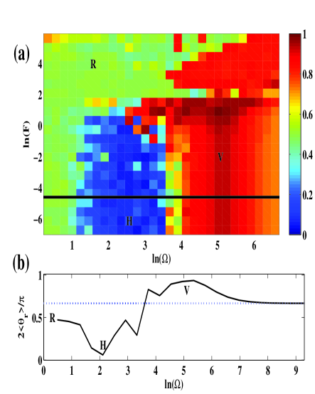
Figure 1: (a) Angular deviation of the bar from horizontal (measured by the reference angle $\theta_{r}$ in units of $\pi/2$, and time-averaged over the final ten cycles) shown as a function of external field parameters (amplitude $F$ and frequency $\Omega$). (b) Same deviation plotted as a function of $\Omega$ with fixed $F=0.01$. The dotted line marks the orientation of the bar at $t=0$.

The equations we just introduced were solved numerically for $n=50$ SP’s in a box with periodic boundary conditions. Typical parameters that roughly reflect the physical charge and mass ratios are obtained by choosing $Q=N=10$. Since our numerical experiments show that the preferred orientation of the bar is not very sensitive to changes in either the frictional effects or the polarizability of the bar itself, we also fix $\gamma_{1}=\gamma_{2}=\gamma_{3}=0.05$ and set $\epsilon(\theta)\equiv 0.2$ (neglecting the angular dependence of the polarizability). Thus, we are left with the two parameters $\alpha$ and $f$ – or, equivalently, $\Omega$ and $F$.

The overall dependence of the bar’s orientation on $\Omega$ and $F$ is shown in Fig. (1a). We characterize the orientation via the reference angle $\theta_{r}$ (the angle $\theta$ mapped onto the first quadrant), which is intuitively more transparent than he usual $P_{2}(\theta)$ Legendre polynomial; $\big{<}\theta_{r}\big{>}$ denotes the average of $\theta_{r}$ over time. In Fig. (1), the color red marks the points in the $\Omega$-$F$ plane where the bar aligns along the direction of the field ($\,\big{<}\theta_{r}\big{>}=\pi/2$, $P_{2}=-0.5\,$), whereas blue indicates the parameter values that lead to anomalous orientation orthogonal to the field ($\,\big{<}\theta_{r}\big{>}=0$, $P_{2}=1\,$). The green points indicate that the time-averaged deviation from the horizontal position is $\pi/4$ ($P_{2}=0.25$), which is the same value that one would get if the orientation of the bar were just a uniformly distributed random variable. Interestingly, the parameter plane is divided in three well-defined regions, with fairly sharp boundaries, where each one of these three behaviors (regular, anomalous and random orientation) is prevalent. For $\ln{F}\lesssim 0$ the choice of orientation is essentially independent of $F$ and depends only on $\Omega$. At higher frequencies the bar aligns with the external field, but if $\ln{\Omega}\lesssim 4$ the preferred orientation changes to orthogonal to the field. At even lower frequencies, however, the external field is not able to orient the bar at all and the angle appears to change randomly. Note that increasing the frequency further ($\ln{\Omega}\gtrsim 6$) results in the bar moving away from a clear vertical orientation (orange region). Dynamically speaking, this is the high-frequency regime where the field polarity changes too rapidly and the bar is minimally affected by both the field and the SP’s. In this regime, as clearly seen from Fig. (1b), the bar remains fixed at the initial orientation. Finally, for $\ln{F}\gtrsim 1$ only the “regular”and ”random” cases arise. We also tested that in the absence of any SP one gets only the vertical orientation (red), as expected.

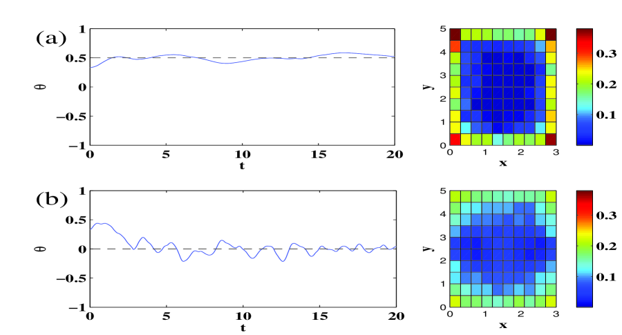
Figure 2: Contrast cases of (a) normal, $F=0.35,\Omega=7.5$ and (b) anomalous, $F=2.72,\Omega=33$, orientation. In each case, the dynamics of the orientation over twenty cycles of the field as well as the density distribution of the secondary (small) particles averaged over a cycle are shown. Note the distinct difference in distributions in the two situations. The dotted lines are intended to guide the eye in terms of final orientation and the angle is measured in units of $\pi$.

In order to gain some insight into the particle dynamics associated with the regular and the anomalous orientation, in Fig. (2) we consider two representative cases and show the time-evolution of $\theta$ (in units of $\pi$) over $20$ cycles of the field. In each case, the parameters considered lie deep in the respective phases in $F$-$\Omega$ space and the dynamics quickly settle the bar into the appropriate alignment. The difference in the distribution of the SP in the two cases is striking. In the regular (vertical orientation) case the particles are essentially confined to the regions along the perimeter of the cell, and especially in the corners. This is in contrast to the anomalous case where the particles inhabit a much larger fraction of the box and are only excluded from two narrow regions immediately surrounding the (large) charges on the bar. Thus, in the high-frequency case the rapid motion of the bar has a cavitating effect, which leads the SP to generate a very flat-bottomed effective potential well; hence, the orientation of the bar is principally determined by the external field as if in a vacuum. By contrast, in the low-frequency case the cloud of SP fills a larger space, contracting and expanding in synchrony with the bar’s oscillations. As a result, the vertical gradient in the cloud’s density produces a net torque on the bar, and the energetically favored configuration is the one in which the PP is kept horizontal by the SP’s effective potential, which prevails on the external potential in orienting of the rod. The fact that the SP are clustered closer to the bar for anomalous orientation provides insight into the relative energetics of the two configurations. The decreased mean spacing between each of the SP and the bar means that this configuration is a more energetic and, in a dynamical sense, unstable one. Finally, in the random phase neither the external field nor the pressure of the cloud is dominant. It is possible that this regime is governed by single SP proximity events rather than collective behavior.

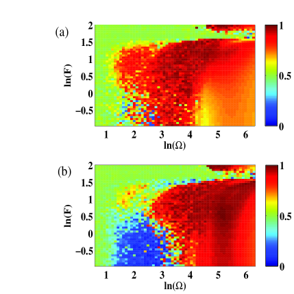
Figure 3: Contrasting cases of (a) rectangular and (b) square aspect ratio. $R$, $V$, and $H$ denote the random, vertical and horizontal phases respectively.

The simulations shown so far have been for a rectangular ($3:5$) box, so one wonders how the phase diagram in $F$-$\Omega$ changes when the aspect ratio is square ($4:4$). As seen from Fig. (3), the anomalous phase vanishes, while the phase boundaries are still visible. This suggests that the distribution of SP no longer generates adequate screening for the anomalous orientation to be attained. The question of why the rectangular case should be reflective of what happens in the experiments is obviously beyond the scope of our simplified single-bar model. We speculate that, in laboratory systems, the interactions among multiple PP in solution favor a mutual alignment of the bars in a lattice structure with spacing consistent with a rectangular cell. We further speculate that such a putative statistical bias towards ”staggering” of the bars may depend only weakly on the concentration of the PP; in fact, the experiments cecco show that PP concentration does not affect the anomalous orientation significantly. These conjectures will be the object of future investigations. Finally, as suggested earlier, the sharp boundaries between the orientation regions in $F$-$\Omega$ space suggest a three-phase diagram akin to what has been seen, for example, in disordered spin systems spinref . There are two distinct ordered phases, corresponding to the normal and anomalous orientation of the rod-like colloid, and a disordered or “glassy” phase corresponding to random orientation. Our dynamical model makes clear the competing influences (frustration) inherent in the system, and this analogy may prove useful in explaining features like re-entrancy visible in the phase diagrams.

References

- (1) W.B. Russell, D.A. Saville and W.R. Schowalter, Colloidal dispersions (Cambridge University Press, Cambridge 1989).
- (2) R.J. Hunter, Foundations of colloid science, (Clarendon Press, Oxford 1987).
- (3) H. Kramer, M. Deggelman, C. Graf, M. Hagenbuchle, C. Johner and R. Weber, Macromolecules 25, 4325 (1992).
- (4) M. E. Cates, J. Phys. II 2, 1109 (1992).
- (5) M. J. Blair and G. N. Patey, J. Chem Phys. 111, 3278 (1999).
- (6) M. Rotunno, T. Bellini, Y. Lansac, and M.A. Glaser, J. Chem Phys. 121, 5541 (2004).
- (7) F. Mantegazza, M. Caggioni, M.L. Jimenez and T. Bellini, Nature Physics 1, 103 (2005).
- (8) T. Bellini, F. Mantegazza, V. Degiorgio, R. Avallone and D.A. Saville, Phys. Rev. Lett. 82, 5160 (1999).
- (9) D. Chowdhury, Spin glasses and other frustrated systems, (Princeton University Press, Princeton 1986).