Abstract

The dynamic evolution at zero temperature of a uniform Ising ferromagnet on a square lattice is followed by Monte Carlo computer simulations. The system always eventually reaches a final, absorbing state, which sometimes coincides with a ground state (all spins parallel), and sometimes does not (parallel stripes of spins $up$ and $down$). We initiate here the numerical study of “Chaotic Time Dependence” (CTD) by seeing how much information about the final state is predictable from the randomly generated quenched initial state. CTD was originally proposed to explain how nonequilibrium spin glasses could manifest equilibrium pure state structure, but in simpler systems such as homogeneous ferromagnets it is closely related to long-term predictability and our results suggest that CTD might indeed occur in the infinite volume limit.

1 Introduction

We consider the Ising model on an $L\times L$ square lattice with periodic boundary conditions. Each site carries a spin either $up$ or $down$, i.e. $S_{ij}=\pm 1$, $i,j=1$, 2 $\dots$ $L$. A pair of neighboring sites has unit energy if the two spin orientations are antiparallel; parallel spins have no energy. The total energy thus ranges from $E=0$ to $2L^{2}$, with the lowest possible energy $E=0$ corresponding to either of the two ground states with all spins either up or down.

A randomly chosen state of this system is stored into the computer memory, and the following dynamic rule is applied to it. A site is chosen at random, and its spin is a candidate to be flipped. If the energy decreases as a result of this flip, then we perform it. Energy increases are not accepted: the chosen spin keeps its current state. If the energy would be unchanged, then the flip is performed with probability 1/2. This procedure is then repeated for another randomly chosen site, and so on.

Physically, this problem corresponds to a sudden quenching from infinite to zero temperature. It was previously studied by measuring the ordinary magnetization, for instance in references [1, 2, 3, 4, 5]. Here we consider it from a completely different point of view: our interest is to study the influence of the starting state on a configuration at a later time $t$.

For each starting state, we perform $D$ independent runs, each corresponding to a different realization of the dynamics (i.e., a different, and also randomly chosen, chronological order of spins selected to be flipped along with a different coin toss for each zero-energy flip encountered). Each step in the time $t$ corresponds to $L^{2}$ flip attempts, i.e. a whole-lattice sweep, on average. The local quantity

$$<S_{ij}>\,\,=\,\,{1\over D}\,\,\sum_{d=1}^{D}\,\,S_{ij}$$ (1)

is calculated at each site $ij\,$, for $t=0$, 1, 2 $\dots$. Furthermore, for each $t$, the global averages

$$Q(t)\,\,=\,\,{1\over L^{2}}\,\,\sum_{ij}\,\,<S_{ij}>$$ (2)

and

$$R(t)\,\,=\,\,{1\over L^{2}}\,\,\sum_{ij}\,\,<S_{ij}>^{2}$$ (3)

are determined, where the sums run over all $L^{2}$ sites.

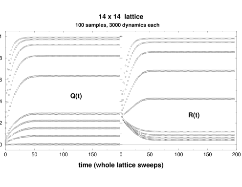
Figure 1: Time functions $Q(t)$ and $R(t)$, Eqs. (2) and (3), averaged over 100 different initial states. Each curve corresponds to a different starting magnetization $m$: exactly $0$ (bottom curves in both sides), $0.01$, $0.02$, $0.03$, $0.04$, $0.10$, $0.15$, $0.20$, $0.25$ and $0.30$ (from bottom to top). At the beginning, $Q(t=0)=m$ and $R(t=0)=1$ in all cases. The error bars lie mostly within the symbols, except for some cases. Note that only for the symmetric case $m=0$ one gets $Q(t)=0$ within the error bars (left). On the other hand, $R(t)$ does not vanish even for this same symmetric case (right). Other lattice sizes, both smaller and larger than $L=14$, follow the same behavior.

In some sense, our approach is the opposite of the process called “damage spreading”, where two slightly different initial states are followed exactly by the same dynamic rule, including the same sequence of spins to be flipped and any other internal or external contingency. Here, we are interested in the effect on the final state of different contingencies occurring during the time evolution, i.e., different chronological orders of the spins to be flipped and different coin tosses for deciding zero-energy flips. Starting from the same initial configuration, equations (1), (2) and (3) compare $D$ parallel, independent evolutions of the same initial state.

Figure 1 shows the time dependences of the global averages for $S=100$ samples, and $D=3000$ different dynamics each. Each sample corresponds to a new starting configuration which is randomly chosen within a fixed value for the magnetization at $t=0$:

$$m\,\,=\,\,{1\over L^{2}}\,\,\sum_{ij}\,\,S_{ij}\,\,\,\,\,\,\,\,{\rm for}\,\,\,\,t=0\,\,\,\,.$$ (4)

In order to prepare the starting state, we choose exactly $(1+m)L^{2}/2$ sites with spins $up$, the remainder $(1-m)L^{2}/2$ sites with spins $down$. Our program stores one spin per bit along a 32-bit computer word, corresponding to 32 different starting states processed at once. For that, we profit from the fast bitwise operations, using techniques described in [6]. As a check, we performed also the same simulations starting from completely random configurations, instead of classifying them according to the magnetization. The results (not shown) are similar to those obtained from $m=0$, but with much larger fluctuations.

One important feature exhibited in Figure 1 is that any small non-zero starting magnetization is enough to break the symmetry: for large enough times, the system saturates on a non-vanishing value for $Q(t)$, always larger than the starting magnetization itself. This is true even for larger lattices (not shown), for which one can better approach the limit $m\to 0$.

As we discuss more fully in the next section when we introduce the notion of “Chaotic Time Dependence” [7], a basic issue we wish to explore concerns the whole set of $D$ distinct dynamical histories starting from the same initial state. In principle, this could be studied by considering $Q(t)$, as $t\to\infty$, without any averaging over $S$ samples (since such averaging would give a quantity essentially the same as the average magnetization) by seeing whether $Q(\infty)$ was nonzero for a nonnegligible fraction of starting states. If somehow all these $D$ distinct histories diverge from each other, how much do they keep in common due to their common starting point? This is the question we are interested in. For initial magnetizations $m\neq 0$, the left part of Figure 1 provides a clear answer. For $m=0$, instead, we look at the quantity $R(t\to\infty)$ which we can average over $S$ samples and ask whether it stays nonzero as system size increases.

Based on the observation that any non-zero starting magnetization is enough to break the $up/down$ symmetry, we conclude that the most interesting case is the initially symmetric situation, i.e. $m=0$ exactly. Thus, hereafter we will treat only this case, fixing attention on the behavior of $R(t)$.

The text is divided into two more sections: first the description of our simulations and the presentation of the results, then our conclusions.

2 Description and Results

A first important observation concerns the absorbing state, i.e. the final distribution of all spins from which no more changes are possible. Before the system reaches this situation, we call it alive, after, it is dead. These terms apply to the whole lattice, not to each spin: the system is dead when no energy decrease or tie can be achieved by flipping any of its spins. As noted earlier, there are only two possible ground states each with energy $E=0$, with all spins either up or down. Both states are clearly absorbing. Our simultations found that in roughly 2/3 of the realizations the system becomes eventually dead in one of these two ground states: we label these realizations with the symbol GS. However, within the remainder 1/3 of the realizations, the system becomes trapped into other absorbing states with $E>0$. The common example is a striped configuration, with alternating stripes of up and down spins, whose widths are larger than one layer. Clearly, this situation does not allow any further change, and the system becomes dead as soon as it is reached: we label these cases with the symbol ST. All of these findings are in agreement with earlier studies [3, 5]. Figure 2 shows two typical countings of GS versus ST situations. Note that the approximate balance 2/3 against 1/3 does not depend on the lattice size: striped configurations always appear, independently of the lattice size.

Figure 2: Statistics of GS realizations, i.e. those for which the absorbing state is a ground state (see first paragraph, Sect. 2). From $D$ (in this case 60) dynamics starting from the same initial state, we record the fraction of GS realizations obtained. The whole procedure is repeated $S$ (in this case 320) times, from which the histogram is constructed.

We discard ST situations, keeping only GS in our statistics. Striped configurations appear as a consequence of the finite lattice size. In an infinite lattice, domains of up or down neighboring spins grow forever; there is zero probability (with respect to either initial configuration or dynamical realization) of the system evolving towards a ‘striped’, or domain wall, state as $t\to\infty$ [9]. This means that any finite region eventually consists of only a single domain (equivalently, after some fixed finite time its spin configuration is GS). Therefore, if our simulations are to provide insights into the infinite lattice situation, it is proper to consider only GS realizations. All other possibilities are consequences of finite size and are thus discarded.

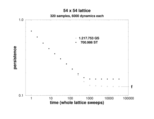
Figure 3: The fraction of never flipped spins (persistence) decays with time as $p\propto t^{-\theta}$. Curves with averages over only GS or only ST realizations are shown. The critical exponent we obtained from GS statistics is $\theta\approx 0.24$ (the same also for other values of $L$ and $D$), in good agreement with earlier studies [10]. Also, the final saturated fraction $f$ scales with the lattice size as $f\propto L^{-\beta}$, with $\beta\approx 0.47$ extracted from our data for $L=10$, 14, 22, 30, 38 and 54.

There is also a ‘practical’ reason for discarding runs terminating in a striped configuration: they are boundary-condition-dependent. Of course, when starting a run, one is not able to predict whether it will evolve into a GS or ST configuration, since the outcome can a priori depend on the dynamical realization. We therefore run each dynamical realization twice. First, we note simply whether for that particular dynamics the system reaches a GS or a ST configuration. By doing this we can perform separate statistics for GS and ST outcomes. As an example, we analyze a quantity defined by Derrida [10]: the fraction of ‘never flipped’ spins as a function of time. This quantity is called persistence, and was shown to display critical behavior, i.e.,

$$p\,\,\propto\,\,t^{-\theta}\,\,\,\,\,\,\,\,,$$ (5)

decaying as a power-law whose critical exponent $\theta$ obeys some universality properties [10]. It is shown in Figure 3. Indeed, the plot obtained from only GS realizations saturates later than the corresponding ST plot, for the same finite lattice size, allowing a better determination of the critical behavior, a practical advantage.

As a byproduct, we also find the further finite-size-scaling relation

$$f(L)\,\,\propto\,\,L^{-\beta}\,\,\,\,\,\,\,\,{\rm with}\,\,\,\,\beta\approx 0.47\,\,\,\,\,\,\,\,,$$ (6)

for the asymptotic saturated persistence $f$, which does not depend on the number $D$ of dynamics.

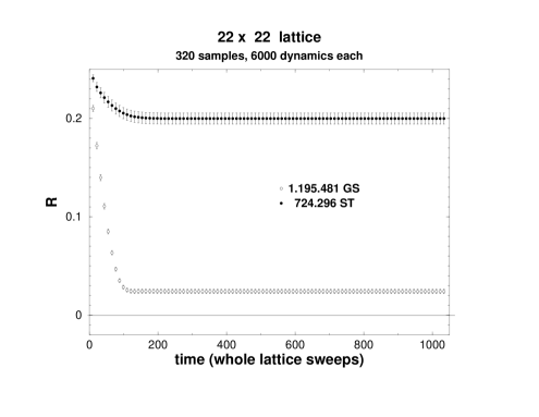
Figure 4: Quantity $R$ as a function of time, averaged over GS (bottom) and ST (top) situations, separately.

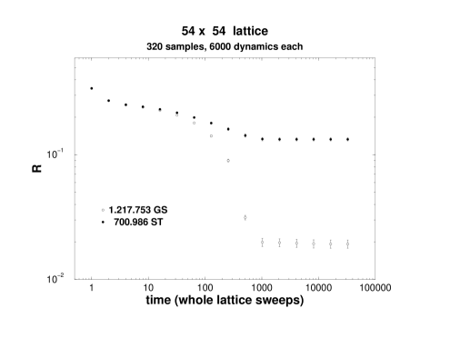
Figure 5: The same as Figure 4, for a larger lattice and using a logarithmic scale.

Figure 4 shows another example, now for the quantity $R$ (cf. Eq. (3)). It saturates in a much smaller value for GS than for ST. This is true also for other lattice sizes, both smaller and larger than $L=22$. Note also the smaller fluctuations (error bars) obtained for GS. Figure 5 shows the same behavior, for a larger lattice, now in logarithmic scale.

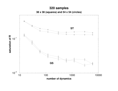
Figure 6: Large-time asymptotic values, $R(t\to\infty)$, as a function of the number $D$ of dynamical runs, for $L=38$ (squares) and $54$ (circles).

Contrary to persistence, the asymptotic value $R(t\to\infty)$ does depend on the number $D$ of dynamics. Figure 6 illustrates the distinct behaviors of $R(t\to\infty)$, for GS and ST realizations, as the number $D$ of dynamical runs increases. For GS the function $R(t)$ is considerably smaller for large enough times.

Let us denote by $R_{L}^{GS}$ the $D\to\infty$, $t\to\infty$ value of $R(t)$, restricted to GS realizations (but otherwise averaged over all initial states). This quantity provides a measure of the information about the final state already contained in a typical, randomly chosen, initial state. It cannot vanish for a fixed finite size $L$ because there are some GS realizations that definitely determine the final state, independent of dynamical realization. Figure 6 does not show significant size dependence of $R(t)$ at large $t$, and hence suggests the possibility that $R_{L}^{GS}$ may not tend to zero as $L\to\infty$. This in turn suggests that the phenomenon of “Chaotic Time Dependence” (CTD) [7] might be occurring.

CTD concerns the large-time predictability of an infinite system based on the randomly generated initial state and not dependent on the realization of the dynamics. CTD means that $<S_{11}>$ at time $t$, averaged over all the dynamics, in the limit $L\to\infty$, does not tend to zero as $t\to\infty$ (and thus forever oscillates between positive and negative values) for typical randomly generated initial states. We note that in principle, CTD could occur even without the nonvanishing of $R_{L\to\infty}^{GS}$ since CTD does not involve any restriction of initial states (to GS) or any averaging over initial states (or equivalently over sites in the lattice). On the other hand, it seems clear that CTD should occur if indeed $R_{L\to\infty}^{GS}\neq 0$.

Figure 7: Number of still alive realizations as a function of time. The inset indicates an exponential asymptotic decay for GS, after a sudden drop at $t_{\rm o}\approx 1000$.

Figure 7 shows the number of still alive realizations as a function of time, again within separated statistics for GS and ST. One observes that some GS realizations are already dead when the first death among ST occurs. Then, within a narrow time interval, all  ST die. On the other hand, after a sudden but not extinguishing drop around $t_{\rm o}\approx 1000$, GS realizations die within a slower rate: some of them survive much more time. The inset shows this last regime for GS, with linear horizontal scale, indicating an exponential decay. The characteristic time when the sudden drop occurs ($t_{\rm o}\approx 1000$ in Figure 7) depends on the lattice size $L$, but not on the number $D$ of dynamics: the larger the lattice size, the later the system enters into the final exponential decay for GS realizations (inset of Figure 7). This regime corresponds to a big sea of $up$ spins with some shrinking islands of neighboring $down$ spins, or vice-versa. It begins at $t_{\rm o}$, when the spontaneous symmetry breaking finally occurs and one of the two possible spin orientations up or down has a majority for the first time: from $t_{\rm o}$ on, this majority fraction increases exponentially fast. An interesting observation is the coincidence of the beginning of this regime with the sudden death of all ST realizations, reinforcing once more our interpretation of ST as mere finite size artifacts: the further exponential decay is aborted for ST realizations, because the minority islands (narrowest stripes) are artificially made stable by the boundary conditions.

Figure 8: Time of first death as function of the lattice size, equation (7).

The characteristic time $t_{\rm o}(L)$ measures the average lifetime for this evolving system. In order to identify its behavior, in the thermodynamic limit $L\to\infty$, we measured for each $L=10$, 14, 22, 30, 38 and 54 the time when the first death occurs among all GS realizations, adopting $S=320$ samples with $D=6000$ dynamics each. The result is a power-law

$$t_{\rm o}(L)\,\,\propto\,\,L^{\alpha}\,\,\,\,\,\,\,\,,$$ (7)

with $\alpha\approx 2$, figure 8. A simple reasoning shows the compatibility of this behavior with that corresponding to persistence, as in Figure 3. At $t=1$ (one complete lattice sweep) the average fraction of non-flipped spins is a constant (numerically 0.708; note also the abrupt drop from $R(0)=1$ to $R(1)\approx 0.25$ in Figure 1), while at the characteristic time $t_{\rm o}$ the final value $f$ is reached (Figure 3). Thus, from equation (5) we can express the corresponding exponent as

$$\theta\,\,=\,\,{\ln({\rm const})-\ln(f)\over\ln(t_{\rm o})-\ln(1)}\,\,\,\,\,\,\,\,{\rm or}\,\,\,\,\,\,\,\,t_{\rm o}\,\,\propto\,\,f^{-1/\theta}\,\,\,\,\,\,\,\,.$$ (8)

Finally, from equation (6) we get

$$t_{\rm o}(L)\,\,\propto\,\,L^{\beta/\theta}\,\,\,\,\,\,\,\,.$$ (9)

By comparing equation (7) with (9), we get the scaling relation

$$\alpha\,\,=\,\,\beta/\theta\,\,\,\,\,\,\,\,,$$ (10)

in agreement with our numerical values $\theta=0.238\pm 0.002$, $\beta=0.466\pm 0.002$ and $\alpha=1.96\pm 0.06$.

An interesting interpretation for the exponent $\alpha=2$ follows. One particular cluster of neighboring parallel spins grows like a diffusive random walk, thus with diameter proportional to $t^{1/2}$. This cluster eventually covers the entire lattice, i.e. $L\propto t_{\rm o}^{1/2}$. Indeed, by following the growth process of the largest cluster just before covering the entire lattice, one observes a typical diffusive process.

3 Conclusions

We have studied the dynamical evolution of $2D$ Ising ferromagnets to explore the extent to which information contained in the randomly generated initial state determines large-time behavior. We did this by comparing different realizations of the dynamical evolution, all starting from the same initial state, i.e., by monitoring the correlations between possible alternative different histories, as functions of time.

Among other findings, we detected two different regimes during the time evolution towards the ground state, by counting how many realizations have already reached it as time goes by. We dicovered the size dependence of the characteristic relaxation time, $t_{\rm o}\propto L^{\beta/\theta}$, where $\theta$ is the Derrida exponent and $\beta$ measures the size scaling of the saturated persistence $f$ (cf. Eq. (6) and Figure 3).

Our most intriguing finding is the suggestion from Figure 6 that the predictability measure $R_{L}^{GS}$ may not vanish in the limit $L\to\infty$ so that even in the infinite volume limit there may be predictability of information about the arbitrarily large time behavior of the system contained in a randomly generated initial state. This will be pursued in a future paper.

Aknowledgements: This work is partially supported by Brazilian agencies FAPERJ and CNPq (process PRONEX-CNPq-FAPERJ/171.168-2003), and by the U.S. National Science Foundation under Grants DMS-01-02587 (CMN) and DMS-01-02541 (DLS). We thank the referees for several useful comments.

References

- [1] C.M. Newman and D.L. Stein, Phys. Rev. Lett. 82, 3944 (1999).
- [2] M.J. de Oliveira and A. Petri, Phil. Mag. B82, 617 (2002).
- [3] V. Spirin, P.L. Krapivsky and S. Redner, Phys. Rev. E65, 016119 (2002).
- [4] M.J. de Oliveira, A. Petri and T. Tom , Europhys. Lett. 65, 20 (2004)
- [5] P. Sundaramurthy and D.L. Stein, J. Phys. A38, 349 (2005).
- [6] P.M.C. de Oliveira, Computing Boolean Statistical Models, World Scientific, New York/London/Singapore (1991).
- [7] C.M. Newman and D.L. Stein, J. Stat. Phys. 94, 709 (1999).
- [8] D. Stauffer, Braz. J. Phys. 30, 787 (2000).
- [9] S. Nanda, C.M. Newman and D.L. Stein, in On Dobrushin’s Way (from Probability Theory to Statistical Physics), R. Minlos, S. Shlosman and Y. Suhov, eds., Amer. Math. Soc. Transl. (2) 198 (2000), pp. 183-194 .
- [10] B. Derrida, A.J. Bray and C. Godreche, J. Phys. A27, 357 (1994); B. Derrida, V. Hakim and V. Pasquier, Phys. Rev. Lett. 75, 751 (1995); B. Derrida, P.M.C. de Oliveira and D. Stauffer, Physica A224, 604 (1996).