Geographical networks evolving with an optimal policy

Abstract

In this article, we propose a growing network model based on an optimal policy involving both topological and geographical measures. In this model, at each time step, a new node, having randomly assigned coordinates in a $1\times 1$ square, is added and connected to a previously existing node $i$, which minimizes the quantity $r_{i}^{2}/k_{i}^{\alpha}$, where $r_{i}$ is the geographical distance, $k_{i}$ the degree, and $\alpha$ a free parameter. The degree distribution obeys a power-law form when $\alpha=1$, and an exponential form when $\alpha=0$. When $\alpha$ is in the interval $(0,1)$, the network exhibits a stretched exponential distribution. We prove that the average topological distance increases in a logarithmic scale of the network size, indicating the existence of the small-world property. Furthermore, we obtain the geographical edge-length distribution, the total geographical length of all edges, and the average geographical distance of the whole network. Interestingly, we found that the total edge-length will sharply increase when $\alpha$ exceeds the critical value $\alpha_{c}=1$, and the average geographical distance has an upper bound independent of the network size. All the results are obtained analytically with some reasonable approximations, which are well verified by simulations.

I Introduction

Since the seminal works on the small-world phenomenon by Watts and Strogatz Watts1998 and the scale-free property by Barabási and Albert Barabasi1999 , the studies of complex networks have attracted a lot of interests within the physical community Albert2002 ; Dorogovtsev2002 ; Newman2003 ; Boccaletti2006 . Most of the previous works focus on the topological properties (i.e. non-geographical properties) of the networks. In this sense, every edge is of length 1, and the topological distance between two nodes is simply defined as the number of edges along the shortest path connecting them. To ignore the geographical effects is reasonable for some networked systems (e.g. food webs Garlaschelli2003 , citation networks Borner2004 , metabolic networks Jeong2000 ), where the Euclidean coordinates of nodes and the lengths of edges have no physical meanings. Yet, many real-life networks, such as transportation networks Sen2003 ; Guimera2005 , the Internet Faloutsos1999 ; Pastor2001 , and power grids Crucitti2004 ; Albert2004 , have well-defined node-positions and edge-lengths. In addition to the topologically preferential attachment introduced by Barabási and Albert Barabasi1999 , some recent works have demonstrated that the spatially preferential attachment mechanism also plays a major role in determining the network evolution Yook2001 ; Barthelemy2003 ; MannaSen .

Very recently, some authors have investigated the spatial structures of the so-called optimal networks Gastner2006 ; Barthelemy2006 . An optimal network has a given size and an optimal linking pattern, and is obtained by a certain global optimization algorithm (e.g. simulated annealing) with an objective function involving both geographical and topological measures. Their works provide some guidelines in network design. However, the majority of real networks are not fixed, but grow continuously. Therefore, to study growing networks with an optimal policy is not only of theoretical interest, but also of practical significance. In this paper, we propose a growing network model, in which, at each time step, one node is added and connected to some existing nodes according to an optimal policy. The degree distribution, edge-length distribution, and topological as well as geographical distances are analytically obtained subject to some reasonable approximations, which are well verified by simulations.

II Model

Consider a square of size $1\times 1$ with open boundary condition, that is, a open set $(0,1)\times(0,1)$ in Euclidean space $\mathbb{R}^{2}$, where “$\times$” signifies the Cartesian product. This model starts with $m$ fully connected nodes inside the square, all with randomly assigned coordinates. Since there exists $m$ nodes initially, the discrete time steps in the evolution are counted as $t=m+1,m+2,\cdots$. Then, at the $t$th time step ($t>m$), a new node with randomly assigned coordinates is added to the network. Rank each previously existing node according to the following measure:

$$\omega_{i}=|\overrightarrow{r_{i}}-\overrightarrow{r_{t}}|^{2}/k_{i}^{\alpha}(t),\texttt{ }i=1,2,\cdots,t-1,$$ (1)

and the node having the smallest $\omega$ is arranged on the top. Here, each node is labelled by its entering time, $\overrightarrow{r_{t}}$ represents the position of the $t$th node, $k_{i}(t)$ is the degree of the $i$th node at time $t$, and $\alpha\geq 0$ is a free parameter. The newly added node will connect to $m$ existing nodes that have the smallest $\omega$ (i.e. on the top of the queue). All the simulations and analyses shown in this paper are restricted to the specific case $m=1$, since the analytical approach is only valid for the tree structure with $m=1$. However, we have checked that all the results will not change qualitatively if $m$ is not too large compared with the network size.

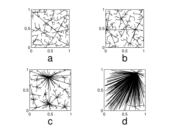
Figure 1: Some network examples for different values of $\alpha$: (a) $\alpha=0$, (b) $\alpha=0.5$, (c) $\alpha=1$, (d) $\alpha=2$. All the four networks are of size $N=300$ and $m=1$.

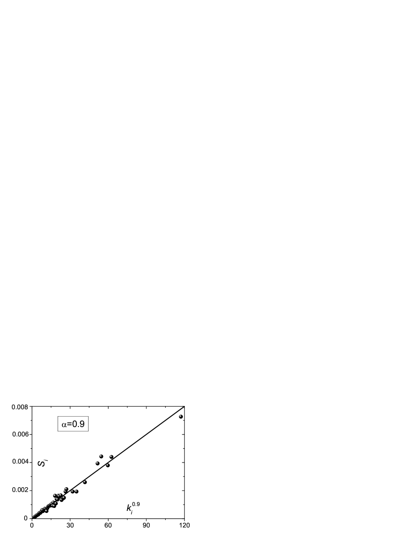
Figure 2: Numerical simulation about the relation between $S_{i}$ and $k_{i}$. The solid line represents the assumption $S_{i}\propto k_{i}^{\alpha}$. In this simulation, we first generate a network of size $N=10000$ by using the present optimal growing policy. To detect $S_{i}$, some test nodes with randomly assigned coordinates are used, and for each test node, following Eq. (1), the existing nodes with minimal $\omega$ is awarded one point. The test node will be removed from the network after testing. The area $S_{i}$ for the $i$th node is approximately estimated as the ratio of the score node $i$ has eventually got after all the testings to the total number of test nodes. The simulation shown here is obtained from 30000 test nodes, and the parameter $\alpha=0.9$ is fixed.

In real geographical networks, short edges are always dominant since constructing long edges will cost more Waxman1988 . On the other hand, connecting to the high-degree nodes will make the average topological distance from the new node to all the previous nodes shorter. These two ingredients are described by the numerator and denominator of Eq. (1), respectively. In addition, the weights of these two ingredients are usually not equal. For example, the airline travellers worry more about the number of sequential connections Guimera2005 , the railway travellers and car drivers consider more about geographical distances Sen2003 , and the bus riders often simultaneously think of both factors Zhang2006 . In the present model, if $\alpha=0$, only the geographical ingredient is taken into account. At another extreme, if $\alpha\rightarrow\infty$, the geographical effect vanishes.

Fig. 1 shows some examples for different values of $\alpha$. When only the geographical ingredient is considered ($\alpha=0$), most edges are very short and the degree distribution is very narrow. In the case of $\alpha=0.5$, the average geographical length of edges becomes longer, and the degree distribution becomes broader. When $\alpha=1$, the scale-free structure emerges and a few hub nodes govern the whole network evolution. As $\alpha$ becomes very large, the network becomes star-like.

III Degree Distribution

At the $t$th time step, there are $t-1$ pre-existing nodes. The square can be divided into $t-1$ regions such that if a new node is fallen inside the $i$th region $S_{i},\texttt{ }i\in\{1,2,\cdots,t-1\}$, the quantity $|\overrightarrow{r_{i}}-\overrightarrow{r_{t}}|^{2}/k_{i}^{\alpha}(t)$ is minimized, thus the new node will attach an edge to the $i$th node. Since the coordinate of the new node is randomly selected inside the square, the probability of connecting with the $i$th node is equal to the area of $S_{i}$. If the positions of nodes are uniformly distributed, statistically, the area of $S_{i}$ is approximately proportional to $k_{i}^{\alpha}(t)$ with a time factor $h(t)$ as $S_{i}\sim h(t)k_{i}^{\alpha}(t)$. Fig. 2 shows the typical simulation results, which strongly support the valid of this assumption. Accordingly, by using the mean-field theory Barabasi1999 , an analytic solution of degree distribution can be obtained. However, when $\alpha>1$, most edges are connected to one single node (see Fig. 1d), so analytic solution is unavailable. Here, we only consider the case of $1\geq\alpha\geq 0$. Assume

$$\sum_{i=1}^{t}k_{i}^{\alpha}(t)\approx At,$$ (2)

where $A$ is a constant that can be determined self-consistently. Using the continuum approximation in time variable $t$, the evolving of node $i$’s degree reads

$${dk_{i}(t)\over dt}=\frac{S_{i}}{\sum^{t}_{i}S_{i}}={k_{i}^{\alpha}\over At},$$ (3)

with the initial condition $k_{i}(i)=1$. The solution is

$$k_{i}(t)=F(t/i),$$ (4)

where

$$F(x)=\left(1+{1-\alpha\over A}\ln(x)\right)^{1/(1-\alpha)}.$$ (5)

Accordingly, the degree distribution can be obtained as

$$P(k)=\frac{1}{t}\sum^{t}_{i=1}\delta(k_{i}(t)-k)={A\over k^{\alpha}e^{{A(k^{1-\alpha}-1)\over 1-\alpha}}}.$$ (6)

The constant $A=\int_{0}^{1}duF^{\alpha}(1/u)$ is determined by the condition $\int kP(k)dk=\langle k\rangle=2$, where $\langle k\rangle=2m=2$ signifies the average degree. The above solution is similar to the one obtained by using the approach of rate equation proposed by Krapivsky et al. krapivsky2000 . In addition, one should note that if $\alpha=1$, the mean-field theory yields a solution $P(k)\sim k^{-3}$, which is comparable to the exact analytic solution $P(k)=4/(k(k+1)(k+2))$.

Clearly, the degree distribution obeys a power-law form at $\alpha=1$, and an exponential form at $\alpha=0$. When $\alpha$ is in the interval $(0,1)$, the networks display the so-called stretched exponential distribution Laherrere1998 : For small $\alpha$, the distribution is close to an exponential one, while for large $\alpha$, it is close to a power law. This result is in accordance with the situation of transportation networks. If only the geographical ingredient is taken into account (e.g. road networks Gastner2006 ), then the degree distribution is very narrow. On the contrary, if the topological ingredient plays a major role (e.g. airport networks Guimera2005 ), then the scale-free property emerges. When both the two ingredients are not neglectable (e.g. bus networks Zhang2006 ), the degree distribution is intervenient between power-law and exponential ones.

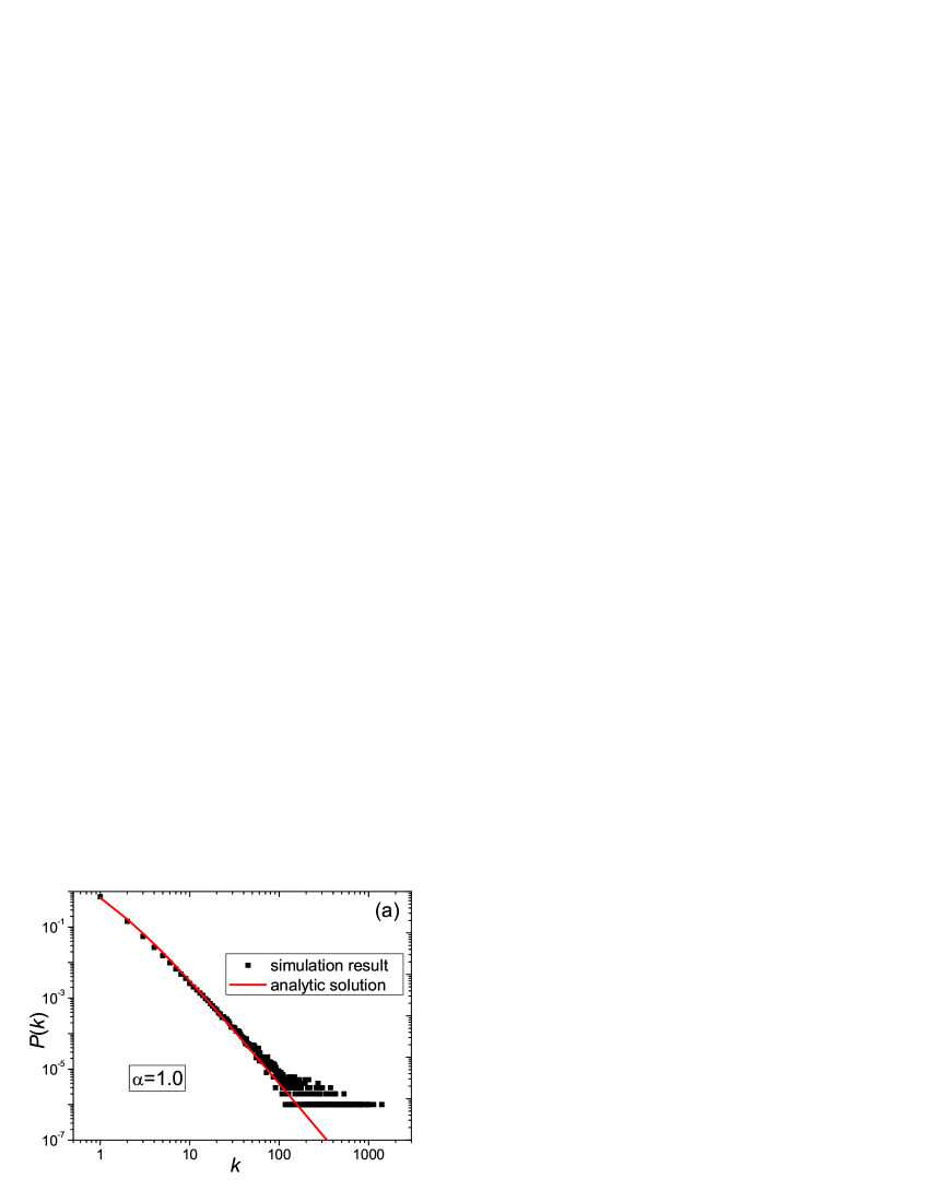
Figure 3: (Color online) The degree distributions for the cases of $\alpha=1$ (a) and $\alpha=0.5$ (b). The black squares and red curves represent simulated and analytic results, respectively. All the data are averaged over $100$ independent runs, with network size $N=10000$ (i.e. $t=10000$) fixed.

Fig. 3 shows the simulation results for $\alpha=1$ and $\alpha=0.5$. The degree distribution follows a power-law form when $\alpha=1$, which well agrees with the analytic solution. In the case of $\alpha=0.5$, the degree distribution is more exponential. However, it is remarkably broader than that of the Erdös-Rényi model Erdos1960 . Note that, the positions of all the nodes are not completely uniformly distributed, which will affect the degree distribution. This effect becomes more prominent when the geographical ingredient plays a more important role (i.e. smaller $\alpha$). Therefore, although the simulation result for $\alpha=0.5$ is in accordance with the analysis qualitatively, the quantitative deviation can be clearly observed.

IV Topological Distance

Denote by $l(i)$ the topological distance between the $i$th node and the first node. By using mathematical induction, we can prove that there exists a positive constant $M$, such that $l(t)<M\texttt{ln}(t)$. This proposition can be easily transferred to prove the inequality $l(t+1)<M\texttt{ln}(t+1)$ under the condition $l(i)<M\texttt{ln}(i)$ for $1\leq i\leq t$. Indeed, since the network has a tree structure, $l(i)$ does not depend on time $t$. Under the framework of the mean field theory, the iteration equation for $l(t)$ reads

$$l(t+1)={\sum_{1\leq i\leq t}k^{\alpha}_{i}(t)l(i)\over At}+1,$$ (7)

with the initial condition $l(1)=0$. Eq. (7) can be understood as follows: At the $(t+1)$th time step, the $(t+1)$th node has probability $k_{i}^{\alpha}(t)/At$ to connect with the $i$th node. Since the average topological distance between the $i$th node and the first node is $l(i)$, the topological distance of the $(t+1)$th node to the first one is $l(i)+1$ if it is connected with the $i$th node. According to the induction assumption,

$$l(t+1)<{M\sum_{1\leq i\leq t}k^{\alpha}_{i}(t)\texttt{ln}(i)\over At}+1.$$ (8)

Note that, statistically, $k_{i}(t)>k_{j}(t)$ if $i<j$, therefore

$$\sum_{1\leq i\leq t}k^{\alpha}_{i}(t)\texttt{ln}(i)<\sum_{1\leq i\leq t}\langle k^{\alpha}(t)\rangle\texttt{ln}(i)=\sum_{1\leq i\leq t}A\texttt{ln}(i),$$ (9)

where $\langle\cdot\rangle$ denotes the average over all the nodes. Substituting inequality (9) into (8), we have

$$l(t+1)<\frac{M}{t}\sum_{1\leq i\leq t}\texttt{ln}(i)+1.$$ (10)

Rewriting the sum in continuous form, we obtain

$$l(t+1)<\frac{M}{t}\int_{1}^{t}\texttt{ln}(x)\texttt{d}x+1<M\texttt{ln}(t+1).$$ (11)

According to the mathematical induction principle, we have proved that the topological distance between the $i$th node and the first node, denoted by $l(i)$, could not exceed the order $O(\texttt{ln}(i))$. For arbitrary nodes $i$ and $j$, clearly, the topological distance between them could not exceed the sum $l(i)+l(j)$, thus the average topological distance $\langle d\rangle$ of the whole network could not exceed the order $O(\texttt{ln}(i))$ either. This topological characteristic is referred to as the small-world effect in network science Watts1998 , and has been observed in a majority of real networks. Actually, one is able to prove that the order of $l(t)$ in the large $t$ limit is equal to $\texttt{ln}(t)$ (see Appendix A for details).

Furthermore, the iteration equation

$$l(t+1)={\sum_{i=1}^{t}f(i)l(i)\over\sum_{i=1}^{t}f(i)}+a(t),$$ (12)

for general functions $f(i)$ and $a(i)$, has the following solution:

$$l(t+1)=l(1)+a(t)+\sum_{j=1}^{t-1}{f(j+1)a(j)\over\sum_{i=1}^{j+1}f(i)}.$$ (13)

For the two special cases of $\alpha=0$ ($a(i)=1$, $f(i)=1$) and $\alpha=1$ ($a(i)=1$, $f(i)=1/\sqrt{i}$), the solutions are simply $l(t)=\texttt{ln}(t)$ and $l(t)=\frac{1}{2}\texttt{ln}(t)$, respectively.

In Fig. 4, we report the simulation results about the average distance $\langle d\rangle$ vs network size $t$. In each case, the data points can be well fitted by a straight line in the semi-log plot, indicating the growth tendency $\langle d\rangle\sim\texttt{ln}(t)$, which agrees well with the analytical solution.

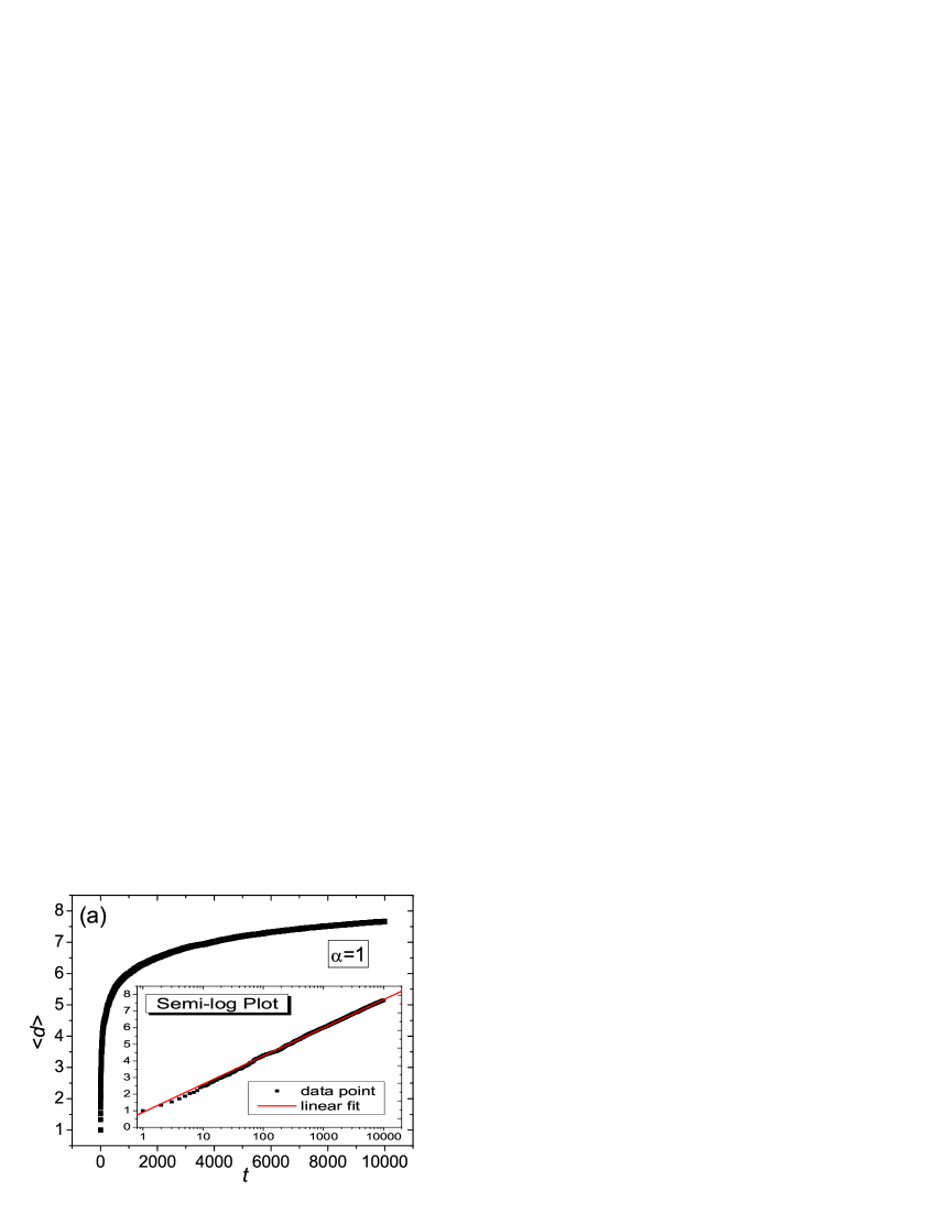
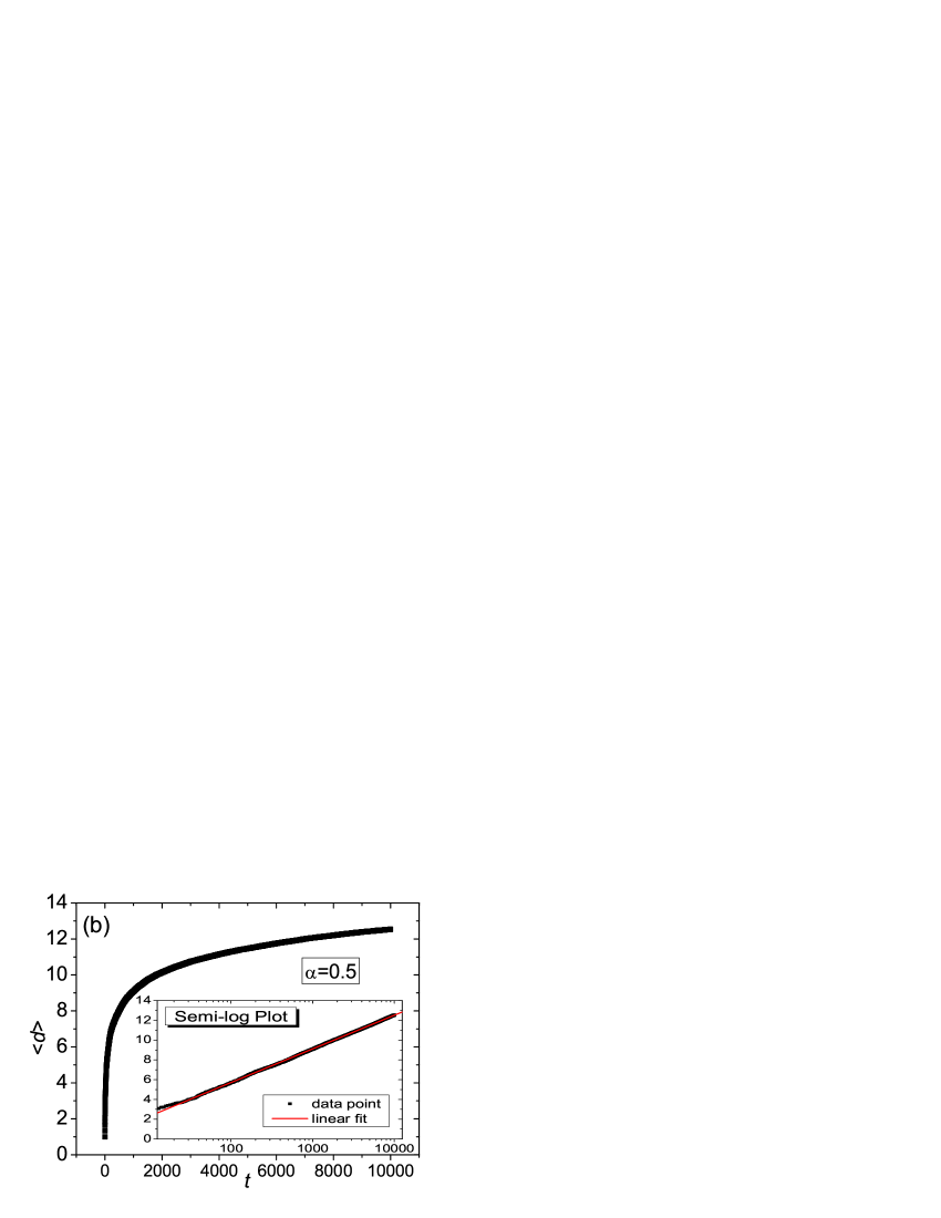
Figure 4: (Color online) The average distance vs network size for the cases of $\alpha=1$ (a) and $\alpha=0.5$ (b). As shown in each inset, the data points can be well fitted by a straight line in the semi-log plot, indicating the growth of the average distance approximately obeys the form $\langle d\rangle\sim\texttt{ln}(t)$. All the data are averaged over $5$ independent runs, where the maximal network size is $N=10000$ (i.e. $t=10000$).

V Edge Length Distribution

Denote by $e_{ij}$ the edge between nodes $i$ and $j$, and the geographical length of edge $e_{ij}$ is $r_{ij}=|\overrightarrow{r_{i}}-\overrightarrow{r_{j}}|$. When the $(N+1)$th node is added to the network, the geographical length of its attached edge approximately obeys the distribution

$$Q(r)=2\pi r\sum_{i=1}^{N}e^{-\pi{r^{2}\over k_{i}^{\alpha}}\sum_{j}k_{j}^{\alpha}},$$ (14)

where $r\ll 1$ in the large $N$ limit. The derivation of this formula is described as follows. The probability of the edge length being between $r$ and $r+dr$ is given by the summation $\sum_{i}Q_{i}dr$, where $Q_{i}dr$ is the probability that $r_{i,N+1}$ falls between $r$ and $r+dr$, and the node $i$ minimizes the quantity $|\overrightarrow{r_{N+1}}-\overrightarrow{r_{i}}|^{2}/k_{i}^{\alpha}$ among all the $N$ previously existing nodes. This probability is approximately given by

$$Q_{i} \approx 2\pi r\prod_{j}\left(1-{\pi r^{2}k_{j}^{\alpha}\over k_{i}^{\alpha}}\right)$$

$$\approx 2\pi re^{-\pi{r^{2}\over k_{i}^{\alpha}}\sum_{j}k_{j}^{\alpha}}.$$

Straightforwardly, the geographical length distribution of the newly added edge at the $t$th time step (the $t$th edge for short) is obtained as

$$P(t,r) = 2\pi r\sum_{i}e^{-\pi{r^{2}\over k^{\alpha}_{i}(t)}\sum_{j}k^{\alpha}_{j}(t)}$$ (16)

$$\approx 2\pi rt\int_{1/t}^{1}due^{-\pi Atr^{2}/F^{\alpha}(1/u)}$$

$$\approx 2\pi rt\int_{0}^{1}due^{-\pi Atr^{2}/F^{\alpha}(1/u)}.$$

The lower boundary in the integral is replaced by 0 in the last step, which is valid only when $\alpha<1$. The cumulative length distribution of the edges at time step $T$ is given by

$$P(r) = \frac{1}{T}\int_{1}^{T}P(t,r)dt$$ (17)

$$= {2\over\pi r^{3}A^{2}T}\int_{0}^{1}duF^{2\alpha}\bigg{[}e^{-\pi Ar^{2}/F^{\alpha}}\left(1+{\pi Ar^{2}\over F^{\alpha}}\right)$$

$$-e^{-\pi ATr^{2}/F^{\alpha}}\left(1+{\pi ATr^{2}\over F^{\alpha}}\right)\bigg{]},$$

where the argument of function $F$ is $1/u$. For $1/\sqrt{T}\ll r\ll 1$, the approximate formula for $P(r)$ reads

$$P(r)\approx{2\over\pi r^{3}A^{2}T}\int_{0}^{1}duF^{2\alpha}\left({1\over u}\right)$$ (18)

and, when $r\ll 1/\sqrt{T}$,

$$P(r)\approx\pi rT.$$ (19)

If $\alpha=1$, the last step in Eq. (16) is invalid but the analytic form for $P(t,r)$ can be directly obtained as

$$P(t,r)=2\pi rt\int_{1/t}^{1}due^{-2\pi tr^{2}\sqrt{u}}$$

$$={1\over\pi r^{3}t}[(1+2\pi r^{2}\sqrt{t})e^{-2\pi r^{2}\sqrt{t}}-(1+2\pi r^{2}t)e^{-2\pi r^{2}t}]$$ (20)

Therefore, when $1/T^{1/4}\ll r\ll 1$, $P(r)$ is approximately given by

$$P(r)\approx{1\over\pi r^{3}T}\ln{C\over 2\pi r^{2}},$$ (21)

where $C$ is a numerical constant, and when $r\ll 1/\sqrt{T}$, $P(r)$ has the same form as that of Eq. (19).

Fig. 5 plots the cumulative edge-length distributions. From this figure, one can see a good agreement between the theoretical and the numerical results. Furthermore, one can calculate the expected value of the $t$th edge’s geographical length, as

$$\overline{r}(t)={\int_{0}^{1}rP(t,r)dr\over\int_{0}^{1}P(t,r)dr}={1\over 2\sqrt{At}}{\int_{0}^{1}duF^{3\alpha/2}(1/u)\over\int_{0}^{1}duF^{\alpha}(1/u)},$$ (22)

which is valid only for sufficiently large $t$ and $\alpha<1$. According to Eq. (22), $\overline{r}(t)$ decreases as $1/\sqrt{t}$ as $t$ increases, which is consistent with the intuition since all the $t$ nodes are embedded into a 2-dimensional Euclidean space. It may also be interesting to calculate the total length $R(t)$ of all the edges at the time step $t$, as

$$R(t)=\sum^{t}_{i=1}\overline{r}(i)\approx\int_{1}^{t}dt^{\prime}\overline{r}(t^{\prime})=\sqrt{{t\over A}}{\int_{0}^{1}duF^{3\alpha/2}(1/u)\over\int_{0}^{1}duF^{\alpha}(1/u)}.$$ (23)

$R(t)$ is proportional to $\sqrt{t}$ for $1>\alpha>0$. When $\alpha>1$, a finite fraction of nodes will be connected with a single hub node and therefore we expect that $R(t)\sim t$ in this case. Therefore, in the large $t$ limit, $R(t)$ will increase quite abruptly when the parameter $\alpha$ exceeds 1. This tendency is indeed observed in our numerical simulations, as shown in Fig. 6.

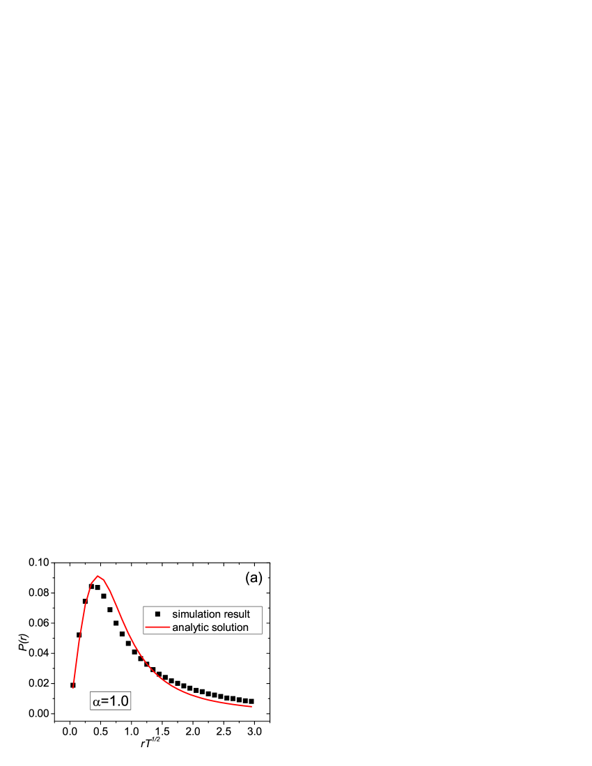
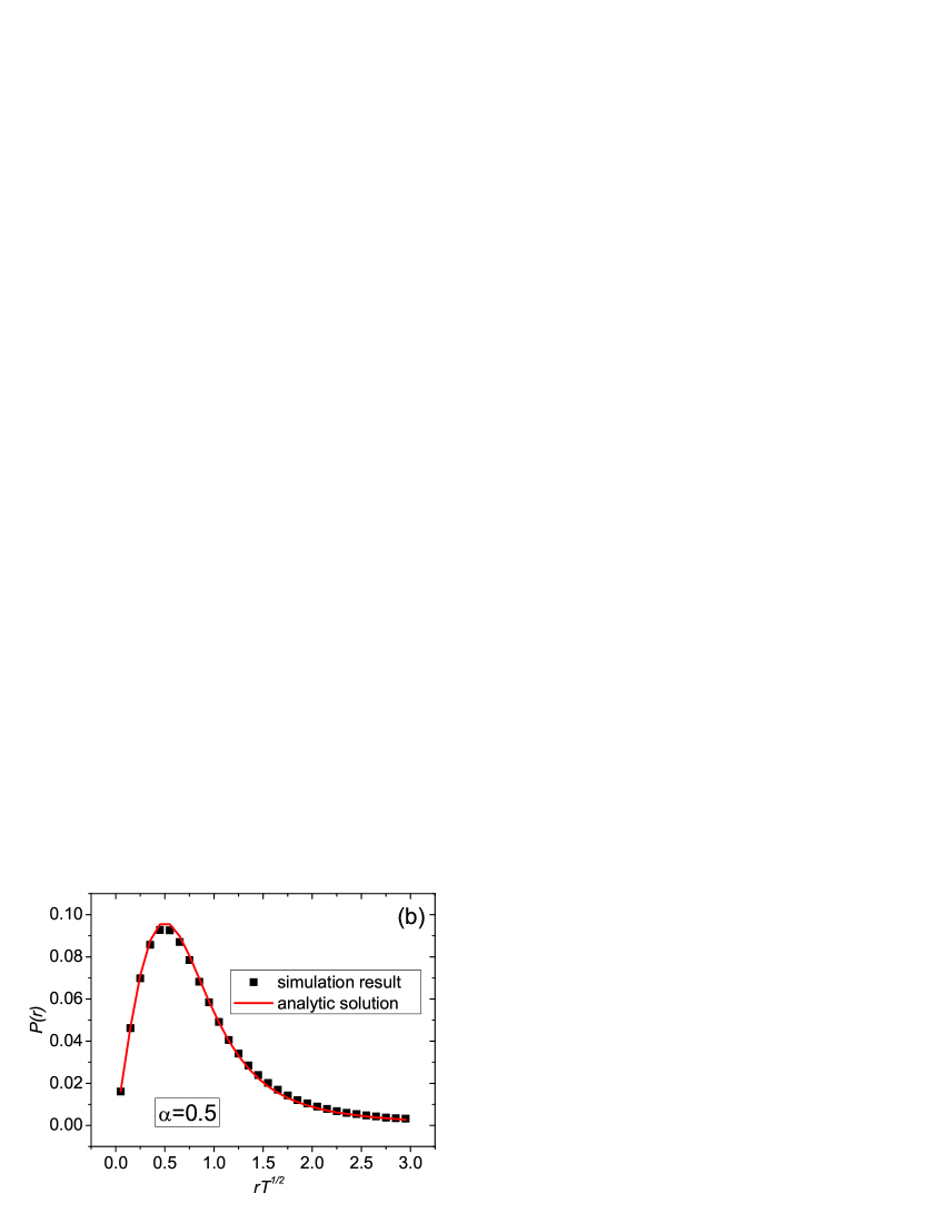
Figure 5: (Color online) The edge length distributions for the cases of $\alpha=1$ (a) and $\alpha=0.5$ (b). The black squares and red curves represent simulation and analytic results, respectively. All the data are averaged over $100$ independent runs, with network size $N=10000$ (i.e. $T=10000$) fixed.

VI Geographical Distance

For an arbitrary path $i_{0}\rightarrow i_{1}\rightarrow\cdots\rightarrow i_{n}$ from node $i_{0}$ to $i_{n}$, the corresponding geographical length is $\sum_{u=0}^{n-1}r_{i_{u}i_{u+1}}$, where $r_{ij}$ denotes the length of edge $e_{ij}$. Accordingly, the geographical distance between two nodes is defined as the minimal geographical length of all the paths connecting them. Now, we calculate the geographical distance $s(i)$ between the $i$th node and the first node. Since our network is a tree graph, $s(i)$ does not depend on time. By using the mean field theory, we have

$$s(t+1)={\sum_{i\leq t}k^{\alpha}_{i}(t)s(i)\over At}+\overline{r}(t+1),$$ (24)

or

$$s(t+1)={1\over A}\int_{1/t}^{1}duF^{\alpha}\left({1\over u}\right)s(ut)+{W\over\sqrt{t+1}},$$ (25)

where, according to Eq. (22),

$$W={1\over 2\sqrt{A}}{\int_{0}^{1}duF^{3\alpha/2}(1/u)\over\int_{0}^{1}duF^{\alpha}(1/u)}.$$ (26)

It is not difficult to see that $s(t)$ has an upper bound as $t$ approaches infinity. One can use the trial solution $s(t)=B-C/t^{\beta}$ to test this conclusion:

$$B-C/(t+1)^{\beta}=B-CE/(At^{\beta})+W/\sqrt{t+1},$$ (27)

where

$$E=\int_{1/t}^{1}duF^{\alpha}(1/u)(1/u^{\beta}).$$ (28)

From Eq. (27), one obtains that $\beta=1/2$.

Similar to the solution of Eq. (13), $s(t)\to 1$ as $t\to\infty$ for $\alpha=0$ and $s(t)\to 1/\sqrt{2}$ as $t\to\infty$ for $\alpha=1$. However, it only reveals some qualitative property, and the exact numbers are not meaningful. This is because the value of $s(t)$ is obtained by the average over infinite configurations for infinite $t$, while in one evolving process $s(t)$ is mainly determined by the randomly assigned coordinates of the $t$th node.

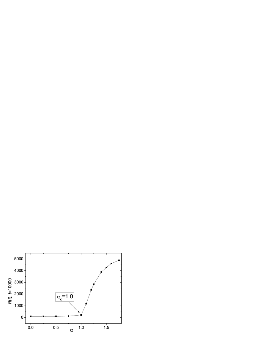
Figure 6: The total edge length $R(t)$ vs parameter $\alpha$ with $t=10000$ fixed. $R(t)$ sharply increases when $\alpha$ exceeds the critical value $\alpha_{c}=1$, which well agrees with the theoretical prediction.

VII Conclusion and Discussion

In many real-life transportation networks, the geographical effect can not be ignored. Some scientists proposed certain global optimal algorithms to account for the geographical effect on the structure of a static network Gastner2006 ; Barthelemy2006 . On the other hand, many real networks grow continuously. Therefore, we proposed a growing network model based on an optimal policy involving both topological and geographical measures. We found that the degree distribution will be broader when the topological ingredient plays a more important role (i.e. larger $\alpha$), and when $\alpha$ exceeds a critical value $\alpha_{c}=1$, a finite fraction of nodes will be connected with a single hub node and the geographical effect will become insignificant. This critical point can also be observed when detecting the total geographical edge-length $R(t)$ in the large $t$ limit. We obtained some analytical solutions for degree distribution, edge-length distribution, and topological as well as geographical distances, based on reasonable approximations, which are well verified by simulations.

Table 1: Empirical degree distributions for geographical transportation networks.

Data-Class	Data-Set	Degree Distribution
Power Grid	Southern California Amaral2000	Exponential
	Whole US Albert2004	$p(k)\sim e^{-0.5k}$
	Italian Crucitti2004	$p(k)\sim e^{-0.55k}$
Subway	Boston Latora2002	Narrow: $k_{\texttt{max}}<10$
	Seoul Chang2006	Narrow: $k_{\texttt{max}}<10$
	Tokyo Chang2006	Narrow: $k_{\texttt{max}}<10$
Railway	Indian Sen2003	$p(k)\sim e^{-0.085k}$
	Switzerland Kurant2006	Exponential
	Central Europe Kurant2006	Exponential
Bus & Tramway	Kraków Sienkiewicz2005	Narrow: $k_{\texttt{max}}=11$
	Warsaw Sienkiewicz2005	Narrow: $k_{\texttt{max}}=13$
	Szczecin Sienkiewicz2005	Narrow: $k_{\texttt{max}}=18$
	Białystok Sienkiewicz2005	Narrow: $k_{\texttt{max}}=19$
Airport	World-Wide Guimera2005	$p(k)\sim k^{-2.0}$
	Chinese Liu2006	$p(k)\sim k^{-2.05}$
	Indian Bagler2004	$p(k)\sim k^{-2.2}$

Although the present model is based on some ideal assumptions, it can, at least qualitatively, reproduce some key properties of the real transportation networks. In Table 1, we list some empirical degree distributions of transportation networks. Clearly, when building a new airport, we tend to firstly open some flights connected with previously central airports which are often of very large degrees. Even though the central airports may be far from the new one, to open a direct flight is relatively convenient since one doesn’t need to build a physical link. Therefore, the geographical effect is very small in the architecture of airport networks, which corresponds to the case of larger $\alpha$ that leads to an approximately power-law degree distribution. For other four cases shown in Table 1, a physical link, which costs much, is necessary if one wants to connect two nodes, thus the geographical effect plays a more important role, which corresponds to the case of smaller $\alpha$ that leads to a relatively narrow distribution.

A specific measure of geographical network is its edge-length distribution. A very recent empirical study Gastner2006 shows that the edge-length distribution of the highly heterogenous networks (e.g. airport networks, corresponding to the present model with larger $\alpha$) displays a single-peak function with the maximal edge-length about five times longer than the peaked value (see Fig. 1c of Ref. Gastner2006 ), while in the extreme homogenous networks (e.g. railway networks, corresponding to the present model with $\alpha\rightarrow 0$), only the very short edge can exist (see Fig. 1a of Ref. Gastner2006 ). These empirical results agree well with the theoretical predictions of the present model. Firstly, when $\alpha$ is obviously larger than zero, the edge-length distribution is single-peaked with its maximal edge-length about six times longer than the peak value (see Fig. 5). And, when $\alpha$ is close to zero, Eq. (17) degenerates to the form

$$P(r)=\frac{2}{\pi r^{3}A^{2}N},$$ (29)

where $N$ denotes the network size. Clearly, in the large $N$ limit, except a very few initially generated edges, only the edge of very small length $r$ can exist.

The analytical approach is only valid for the tree structure with $m=1$. However, we have checked that all the results will not change qualitatively if $m$ is not too large compared with the network size. Some analytical methods proposed here are simple but useful, and may be applied to some other related problems about the statistical properties of complex networks. For example, a similar (but much simpler) approach, taken in section 4, can also be used to estimate the average topological distance for some other geographical networks Zhou2005 ; ZhangZZ2006 .

Finally, it is worthwhile to emphasize that, the geographical effects should also be taken into account when investigating the efficiency (e.g. the traffic throughput Yan2006 ) of transportation networks. Very recently, some authors started to consider the geographical effects on dynamical processes, such as epidemic spreading Xu2006 and cascading Huang2006 , over scale-free networks. We hope the present work can further enlighten the readers on this interesting subject.

Appendix A The solution of $l(t)$

Substituting Eq. (4) into Eq. (7), one obtains that

$$l(t+1)={1\over A}\int_{1/t}^{1}duF^{\alpha}\left({1\over u}\right)l(ut)+1.$$ (30)

Then, define

$$B=A\left\{\int_{0}^{1}duF^{\alpha}(1/u)\ln(1/u)\right\}^{-1}.$$ (31)

We next prove that $l(t)\approx B\ln t$ in the large $t$ limit by using mathematical induction. Suppose for sufficiently large $t$, all $l(i)$ are less than $C\ln(i)$ for $i\leq t$ with $C$ being a constant greater than $B$. Then, from Eq. (A1), we have

$$l(t+1) \leq {C\over A}\int_{1/t}^{1}duF^{\alpha}\left({1\over u}\right)\ln(ut)+1$$ (32)

$$= -{C\over B}+1+M\ln(t)+O\left({1\over t}\right)$$

$$\leq C\ln(t+1)$$

Therefore, $l(i)\leq C\ln(i)$ for all $i$. Similarly, suppose for sufficiently large $t$, all $l(i)$ are greater than $Q\ln i$ for $i\leq t$ with $Q$ being a constant less than $B$. Then, from Eq. (A1), we have

$$l(t+1) \geq {Q\over A}\int_{1/t}^{1}duF^{\alpha}\left({1\over u}\right)\ln(ut)+1$$ (33)

$$= -{Q\over B}+1+M\ln(t)+O\left({1\over t}\right)$$

$$\geq Q\ln(t+1).$$

Therefore, $l(i)\geq Q\ln(i)$ for all $i$.

Combine both the upper bound (A3) and lower bound (A4), we obtain the order of $l(t)$ in the large $t$ limit, as $l(t)\approx B\ln(t)$.

References

- (1) D. J. Watts, and S. H. Strogatz, Nature 393, 440 (1998).
- (2) A. -L. Barabási, and R. Albert, Science 286, 509 (1999); A. -L. Barabási, R. Albert, and H. Jeong, Physica A 272, 173 (1999).
- (3) R. Albert, and A. -L. Barabási, Rev. Mod. Phys. 74, 47 (2002).
- (4) S. N. Dorogovtsev, and J. F. F. Mendes, Adv. Phys. 51, 1079 (2002).
- (5) M. E. J. Newman, SIAM Review 45, 167 (2003).
- (6) S. Boccaletti, V. Latora, Y. Moreno, M. Chavez, and D. -U. Hwang, Phys. Rep. 424, 175 (2006).
- (7) D. Garlaschelli, G. Caldarelli, and L. Pietronero, Nature 423, 165 (2003).
- (8) K. Börner, J. T. Maru, and R. L. Goldstone, Proc. Natl. Acad. Sci. U.S.A. 101, 5266 (2004).
- (9) H. Jeong, B. Tombor, R. Albert, Z. N. Oltvai, and A. -L. Barabási, Nature 407, 651 (2000).
- (10) P. Sen, S. Dasgupta, A. Chatterjee, P. A. Sreeram, G. Mukherjee, and S. S. Manna, Phys. Rev. E 67, 036106 (2003).
- (11) A. Brrrat, M. Barthélemy, R. Pastor-Satorras, and A. Vespignani, Proc. Natl. Acad. Sci. U.S.A. 101, 3747 (2004); R. Guimerà, S. Mossa, A. Turtschi, and L. A. N. Amaral, Proc. Natl. Acad. Sci. U.S.A. 102, 7794 (2005).
- (12) M. Faloutsos, P. Faloutsos, and C. Faloutsos, Comput. Commun. Rev. 29, 251 (1999).
- (13) R. Pastor-Satorras, A. Vázquez, and A. Vespignani, Phys. Rev. Lett. 87, 258701 (2001).
- (14) R. Crucitti, V. Latora, and M. Marchiori, Physica A 338, 92 (2004).
- (15) R. Albert, I. Albert, and G. L. Nakarado, Phys. Rev. E 69, 025103 (2004).
- (16) S. H. Yook, H. Jeong, and A. -L. Barabási, Proc. Natl. Acad. Sci. U.S.A. 99, 13382 (2001).
- (17) M. Barthélemy, Europhys. Lett. 63, 915 (2003); C. Herrmann, M. Barthélemy, and P. Provero, Phys. Rev. E 68, 026128 (2003).
- (18) S. S. Manna and P. Sen, Phys. Rev. E 66,066114 (2002); P. Sen, K. Banerjee, and T. Biswas, Phys. Rev. E 66, 037102 (2002); P. Sen and S. S. Manna, Phys.Rev. E 68, 026104 (2003); S. S. Manna, G. Mukherjee, and P. Sen, Phys. Rev. E 69, 017102 (2004); G. Mukberjee, and S. S. Manna, Phys. Rev. E 74, 036111 (2006).
- (19) M. T. Gastner, and M. E. J. Newman, Eur. Phys. J. B 49, 247 (2006).
- (20) M. Barthélemy, and A. Flammini, e-print arXiv: physics/0601203.
- (21) B. M. Waxman, IEEE J. Selected Areas Comm. 6, 1617 (1988).
- (22) P. -P. Zhang, K. Chen, Y. He, T. Zhou, B. -B. Su, Y. -D. Jin, H. Chang, Y. -P. Zhou, L. -C. Sun, B. -H. Wang, D. -R. He, Physica A 360, 599 (2006).
- (23) P.L. Krapivsky, S. Redner, and F. Leyvraz, Phys. Rev. Lett. 85, 4629 (2000); P.L. Krapivsky, and S. Redner, Phys. Rev. E 63, 066123 (2001).
- (24) J. Laherrere, and D. Sornette, Eur. Phys. J. B 2, 525 (1998).
- (25) P. Erdös, and A. Rényi, Publ. Math. Inst. Hung. Acad. Sci. 5, 17 (1960).
- (26) L. A. N. Amaral, A. Scala, M. Barthélemy, and H. E. Stanley, Proc. Natl. Acad. Sci. U.S.A. 97, 11149 (2000); S. H. Strogatz, Nature 410, 268 (2001).
- (27) L. A. Braunstein, S. V. Buldyrev, R. Cohen, S. Havlin, and H. E. Stanley, Phys. Rev. Lett. 91, 168701 (2003).
- (28) V. Latora, and M. Marchiori, Physica A 314, 109 (2002).
- (29) K. H. Chang, K. Kim, H. Oshima, and S. -M. Yoon, J. Korean Phys. Soc. 48, S143 (2006).
- (30) M. Kurant, and P. Thiran, Phys. Rev. Lett. 96, 138701 (2006); Phys. Rev. E 74, 036114 (2006).
- (31) J. Sienkiewicz, and J. A. Hołyst, Phys. Rev. E 72, 046127 (2005).
- (32) H. -K. Liu, and T. Zhou, Acta Physica Sinica (to be published).
- (33) G. Bagler, e-print cond-mat/0409773.
- (34) T. Zhou, G. Yan, and B. -H. Wang, Phys. Rev. E 71, 046141 (2005); Z. -M. Gu, T. Zhou, B. -H. Wang, G. Yan, C. -P. Zhu, and Z. -Q. Fu, Dyn. Contin. Discret. Impuls. Syst. Ser. B-Appl. Algorithms 13, 505 (2006).
- (35) Z. -Z. Zhang, L. -L. Rong, and F. Comellas, Physica A 364, 610 (2006); Z. -Z. Zhang, L. -L. Rong, and F. Comellas, J. Phys. A 39, 3253 (2006).
- (36) G. Yan, T. Zhou, B. Hu, Z. -Q. Fu, and B. -H. Wang, Phys. Rev. E 73, 046108 (2006); T. Zhou, G. Yan, B. -H. Wang, Z. -Q. Fu, B. Hu, C. -P. Zhu, and W. -X. Wang, Dyn. Contin. Discret. Impuls. Syst. Ser. B-Appl. Algorithms 13, 463 (2006).
- (37) X. -J. Xu, Z. -X. Wu, and G. Chen, e-print arXiv: physics/0604187; X. -J. Xu, W. -X. Wang, T. Zhou, and G. Chen, e-print arXiv: physics/0606256.
- (38) L. Huang, L. Yang, and K. Yang, Phys. Rev. E 73, 036102 (2006).