Abstract

In this paper, a spatially dispersive finite-difference time-domain (FDTD) method to model wire media is developed and validated. Sub-wavelength imaging properties of the finite wire medium slabs are examined. It is demonstrated that the slab with its thickness equal to an integer number of half-wavelengths is capable of transporting images with sub-wavelength resolution from one interface of the slab to another. It is also shown that the operation of such transmission devices is not sensitive to their transverse dimensions, which can be made even comparable to the wavelength. In this case, the edge diffractions are negligible and do not disturb the image formation.

OCIS codes: (120.6640) Superresolution, (110.2990) Image formation theory, (260.2030) Dispersion.

1 Introduction

The conventional imaging systems operate only with propagating harmonics emitted by a source, since the spatial harmonics carrying sub-wavelength information (evanescent waves) exhibit exponential decay in free space. This is why the resolution of common imaging systems is restricted by the diffraction limit: The details smaller than the wavelength can not be resolved. A realization of imaging with sub-wavelength resolution may enable breakthrough in creation of future imaging devices at microwave, sub-millimeter, terahertz, infrared and optical frequency ranges, and can lead to significant progress of emerging technologies. For example, the sub-wavelength imaging can be used in optical industry for enlargement of the capacity of optical drives (DVD), in antenna industry and in near field microscopy for improvement of near field scanners, in medicine for magnetic resonance imaging (MRI) and terahertz imaging, etc.

An idea to overcome the diffraction limit was first suggested by Sir John Pendry in his seminal paper [1]. It was proposed to use left-handed materials, isotropic media with both negative permittivity and permeability [2]. A planar slab of such a material provides an opportunity for imaging with sub-wavelength resolution due to the effects of negative refraction and amplification of evanescent waves. However, it is still problematic to manufacture left-handed media since it requires to artificially create negative permeability. Currently available designs of left-handed media (at both microwave and optical frequency ranges) are very lossy that restrict and even prevent their sub-wavelength imaging applications. There is an alternative approach for sub-wavelength imaging which does not involve either left-handed media or effects of negative refraction and amplification of evanescent waves. This new regime was recently suggested in the paper [3] where it was named canalization. The idea is that both propagating and evanescent harmonics of a source can be transformed into the propagating waves inside a slab of certain materials. Then, these propagating modes are capable of transporting sub-wavelength images from one interface of the slab to another. The source has to be placed very close to the front interface of the slab in order to avoid deterioration of the sub-wavelength details in the free space. A reflection from the slab can be minimized by appropriate choice of its thickness. If the slab is tuned for Fabry-Perot resonance then the reflection from its interface is negligibly small for all angles of incidence including complex ones. This allows to avoid harmful interactions between the source and the slab which can disturb the image. An appropriate material for operation in the canalization regime should have a flat isofrequency contour, or in other words it should support waves traveling in a certain direction with the fixed phase velocity for any transverse wave vector. The materials which fulfil this requirement are available at both microwave [3, 4, 5] and optical [6] frequency ranges. The most interesting opportunity was suggested in [5] where the wire medium, a regular array of parallel metallic wires [7] was used. Originally, it was expected that the transmission devices formed by the wire media would operate only at microwave frequencies where the most of the metals behave as ideal conductors. However, recently it has been proposed to use the same structures for sub-wavelength imaging at terahertz and infrared frequency bands where metals reveal their plasma-like properties [8].

In the present paper we study the performance of sub-wavelength imaging by transmission devices formed by the wire medium at microwave frequencies. The finite-sized planar slabs of wire medium excited by sub-wavelength sources are modeled using the finite-difference time-domain (FDTD) method. The wire medium is treated as a bulky material other than an actual periodic array of wires in [5].

2 Spatial dispersion in the wire medium

The wire medium is an artificial material formed by parallel perfect- conducting wires arranged into a rectangular lattice (see Fig. 1).

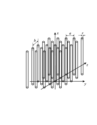
Fig. 1: The wire medium: a rectangular lattice of parallel ideally conducting thin wires.

This medium has been known as an artificial dielectric with plasma-like properties at microwave frequencies for a long time [9, 10, 11], but only recently it was shown that the wire medium has strong spatial dispersion [7]. In other words, the wire medium is a non-local material and in the spectral domain it can not be described using only frequency dependent permittivity tensor. The permittivity tensor of the wire medium depends also on the wave vector. In this paper we will use the following expression for the permittivity tensor derived in [7]:

$$\overline{\overline{\epsilon}}(\omega,{\bf q})=\varepsilon(\omega,q_{x}){\bf x}{\bf x}+{\bf y}{\bf y}+{\bf z}{\bf z},\qquad\varepsilon(\omega,q_{x})=1-\frac{k_{p}^{2}}{k^{2}-q_{x}^{2}},$$ (1)

where the $x$-axis is oriented along wires, $q_{x}$ is the $x$-component of the wave vector ${\bf q}$, $k=\omega/c$ is the wave number of the free space, $c$ is the speed of light, and $k_{p}$ is the wave number corresponding to the plasma frequency of the wire medium. The wave number $k_{p}$ depends on the lattice periods $a$ and $b$, and on the radius of wires $r$ [12]:

$$k_{p}^{2}=\frac{2\pi/(ab)}{\log\frac{\sqrt{ab}}{2\pi r}+F(a/b)},\qquad F(\xi)=-\frac{1}{2}\log\xi+\sum\limits_{n=1}^{+\infty}\left(\displaystyle\frac{\mbox{coth}(\pi n\xi)-1}{n}\right)+\frac{\pi}{6}\xi.$$ (2)

For the case of the square grid ($a=b$), $F(1)=0.5275$ and the expression (2) reduces to

$$k_{p}^{2}=\frac{2\pi/a^{2}}{\ln\frac{a}{2\pi r}+0.5275}.$$ (3)

The expression (1) for the permittivity tensor of the wire medium is valid if the wires are thin as compared to the lattice periods (when the polarization across the wires is negligibly small as compared to the longitudinal polarization) and if the lattice periods are much smaller than the wavelength (when the wire medium can be homogenized).

The wire medium supports three different types of modes, in contrast to the usual uniaxial dielectrics which only support two types of modes: ordinary and extraordinary:

• TE modes (ordinary modes, transverse electric field with respect to the wires), the waves which are polarized across the wires and do not induce any currents along the wires. In the thin wire approximation one can regard these as the modes which travel in the free space and do not interact with the wires.

• TM modes (extraordinary modes, transverse magnetic field with respect to the wires), the waves which correspond to nonzero currents in the wires and nonzero electric field along the wires. At the frequencies below the plasma frequency, these waves are evanescent.

• TEM modes (transmission-line modes, transverse electric and magnetic field with respect to the wires), the waves with nonzero currents in the wires, but with zero electric field along the wires. These modes travel with the speed of light along the wires ($q_{x}=\pm k$) and can have any wave vector in the transverse direction. Effectively, these waves correspond to the modes of a multi-conductor transmission line formed by the wires, and enable us to use wire medium for realization of the canalization regime.

The presence of TEM (transmission-line) mode provides an evidence of the strong spatial dispersion in the wire media. Usually, effects of the spatial dispersion can be observed in any periodical structure at the frequencies corresponding to the spatial resonances when the wavelength in the free space is comparable with the period of the structure, as in usual photonic and electromagnetic crystals, or when the wavelength in the crystal becomes comparable with the period of the structure due to the resonant behavior of inclusions, like in the case of resonant artificial dielectrics or photonic crystals made from self-resonant inclusions. The wire medium is a unique material where the spatial dispersion is observed at very low frequencies and without any resonant effects.

3 Spatially dispersive FDTD method for numerical modeling of the wire medium

The FDTD method for numerical solutions of Maxwell’s equations was first proposed by Yee in 1966 [13]. The method is based on an iterative process which allows to obtain the electromagnetic fields throughout the computational domain at a certain time step in terms of the fields at the previous time steps using a set of updating equations [14]. The typical discretization scheme involves forming a dual-electric-magnetic field grid with electric and magnetic cells spatially and temporally offset from each other. The main advantages of the FDTD method are its simplicity, effectiveness and accuracy as well as the capability of modeling frequency dispersive and anisotropic materials. The FDTD method has been widely used for modeling of various structures which include components formed by materials with complex electromagnetic properties: frequency dispersive and anisotropic dielectrics and magnetics, bi-anisotropic media, ferrites, nonlinear materials, left-handed media and photonic crystals, etc. The simulations of materials with complex inner geometries can be performed either by modeling actual structures or through the effective medium approach (if applicable). The second possibility allows to dramatically decrease complexity of calculations and save computational time.

In spite of the considerable number of complex electromagnetic media modeled using the FDTD method, still there is a certain incompleteness in consideration. Being focused on the frequency dispersion effects, researchers have practically ignored the spatial dispersion. According to our knowledge, so far no FDTD modeling of spatially dispersive materials has been done. Probably, the lack of attention to the spatial dispersion effects is caused by two following reasons. The first reason is that it is widely assumed that the spatial dispersion effects are usually quite weak and can be neglected. However, this is not true: there is a number of complex materials in which the spatial dispersion effects are strong and play dominant roles in determination of their electromagnetic properties. One example of such materials, the wire medium, is considered in this paper. The second possible reason why the spatial dispersion effects did not attract much attention of researchers is a complexity in description of the spatial dispersion effects. The analytical expressions which describe spatial dispersion for particular materials are generally not available in contrast to the numerous analytical models which describe the frequency dispersion effects. The wire medium is an exception form this rule. The spatial dispersion effects in this material can be described by simple analytical formula (1).

In the present paper, the wire medium is modeled as a frequency and spatially dispersive dielectric with permittivity tensor (1). Both frequency and spatial dispersion effects are taken into account in FDTD modeling using an auxiliary differential equation method. At the spectral ($\omega$-${\bf q}$) domain, the relation between the electric flux density ${\bf D}$ and the electric field intensity ${\bf E}$ in the wire medium is following:

$${\bf D}(\omega,{\bf q})=\varepsilon_{0}\overline{\overline{\varepsilon}}(\omega,{\bf q}){\bf E}(\omega,{\bf q}),$$ (4)

where $\varepsilon_{0}$ is permittivity of the free space and $\overline{\overline{\varepsilon}}(\omega,{\bf q})$ is given by (1). The substitution of (1) into (4) gives:

$$\left(k^{2}-q^{2}_{x}\right)D_{x}(\omega,{\bf q})+\left(q^{2}_{x}-k^{2}+k^{2}_{p}\right)\varepsilon_{0}E_{x}(\omega,{\bf q})=0,$$ (5)

$$D_{y}(\omega,{\bf q})=\varepsilon_{0}E_{y}(\omega,{\bf q}),~{}~{}~{}~{}D_{z}(\omega,{\bf q})=\varepsilon_{0}E_{z}(\omega,{\bf q}).$$ (6)

Applying inverse Fourier transformation to Eqs. (5) and (6) we obtain the constitutive relations in the time-space ($t$-${\bf r}$) domain in the following form:

$$\left(\frac{\partial^{2}}{\partial x^{2}}-\frac{1}{c^{2}}\frac{\partial^{2}}{\partial t^{2}}\right)D_{x}(t,{\bf r})+\left(\frac{1}{c^{2}}\frac{\partial^{2}}{\partial t^{2}}-\frac{\partial^{2}}{\partial x^{2}}+k^{2}_{p}\right)\varepsilon_{0}E_{x}(t,{\bf r})=0,$$ (7)

$$D_{y}(t,x)=\varepsilon_{0}E_{y}(t,{\bf r}),\qquad D_{z}(t,x)=\varepsilon_{0}E_{z}(t,{\bf r}).$$ (8)

The FDTD simulation domain is represented by an equally spaced three-dimensional grid with periods $\Delta_{x}$, $\Delta_{y}$ and $\Delta_{z}$ along $x$-, $y$- and $z$-directions, respectively. The time step is $\Delta_{t}$. For discretization of (7), we use the central finite difference operators in both time $\delta^{2}_{t}$ and space $\delta^{2}_{x}$, defined as in [15]:

$$\frac{\partial^{2}}{\partial t^{2}}\rightarrow\frac{\delta^{2}_{t}}{\Delta^{2}_{t}},\qquad\delta^{2}_{t}F|^{n}_{m_{x},m_{y},m_{z}} \equiv F|^{n+1}_{m_{x},m_{y},m_{z}}-2F|^{n}_{m_{x},m_{y},m_{z}}+F|^{n-1}_{m_{x},m_{y},m_{z}};$$

$$\frac{\partial^{2}}{\partial x^{2}}\rightarrow\frac{\delta^{2}_{x}}{\Delta^{2}_{x}},\qquad\delta^{2}_{x}F|^{n}_{m_{x},m_{y},m_{z}} \equiv F|^{n}_{m_{x}+1,m_{y},m_{z}}-2F|^{n}_{m_{x},m_{y},m_{z}}+F|^{n}_{m_{x}-1,m_{y},m_{z}};$$ (9)

where $F$ represents $D_{x}$ or $E_{x}$; $m_{x},m_{y},m_{z}$ are indices corresponding to a certain discretization point in the FDTD domain, and $n$ is a number of the time steps. The discretization of Eq. (8) leads to the standard updating equations. The discretized Eq. (7) reads

$$\left(\frac{\delta^{2}_{x}}{\Delta^{2}_{x}}-\frac{1}{c^{2}}\frac{\delta^{2}_{t}}{\Delta^{2}_{t}}\right)D_{x}+\left(\frac{1}{c^{2}}\frac{\delta^{2}_{t}}{\Delta^{2}_{t}}-\frac{\delta^{2}_{x}}{\Delta^{2}_{x}}+k^{2}_{p}\right)\varepsilon_{0}E_{x}=0,$$ (10)

and it can be rewritten in the open form as:

$$\!\biggl{(}\frac{D_{x}|^{n}_{m_{x}+1,m_{y},m_{z}}-2D_{x}|^{n}_{m_{x},m_{y},m_{z}}+D_{x}|^{n}_{m_{x}-1,m_{y},m_{z}}}{\Delta^{2}_{x}}-\frac{1}{c^{2}}\frac{D_{x}|^{n+1}_{m_{x},m_{y},m_{z}}-2D_{x}|^{n}_{m_{x},m_{y},m_{z}}+D_{x}|^{n-1}_{m_{x},m_{y},m_{z}}}{\Delta^{2}_{t}}\biggr{)}$$ (11)

$$\!\!\!\!\!\!\!\!\!\!\!\!\!\!\!\!+\varepsilon_{0}\biggl{(}\frac{1}{c^{2}}\frac{E_{x}|^{n+1}_{m_{x},m_{y},m_{z}}-2E_{x}|^{n}_{m_{x},m_{y},m_{z}}+E_{x}|^{n-1}_{m_{x},m_{y},m_{z}}}{\Delta^{2}_{t}}-\frac{E_{x}|^{n}_{m_{x}+1,m_{y},m_{z}}-2E_{x}|^{n}_{m_{x},m_{y},m_{z}}+E_{x}|^{n}_{m_{x}-1,m_{y},m_{z}}}{\Delta^{2}_{x}}$$

$$~{}~{}+k^{2}_{p}E_{x}|^{n}_{m_{x},m_{y},m_{z}}\biggr{)}=0.$$

Therefore, the updating equation for $E_{x}$ in terms of $E_{x}$ and $D_{x}$ at the previous time steps is obtained as follows:

$$E_{x}|^{n+1}_{m_{x},m_{y},m_{z}}=\frac{c^{2}\Delta^{2}_{t}}{\Delta^{2}_{x}}\left(E_{x}|^{n}_{m_{x}+1,m_{y},m_{z}}+E_{x}|^{n}_{m_{x}-1,m_{y},m_{z}}\right)+\left(2-\frac{2c^{2}\Delta^{2}_{t}}{\Delta^{2}_{x}}-c^{2}\Delta^{2}_{t}k^{2}_{p}\right)E_{x}|^{n}_{m_{x},m_{y},m_{z}}$$ (12)

$$~{}~{}~{}~{}~{}~{}~{}~{}~{}~{}~{}~{}~{}~{}-E_{x}|^{n-1}_{m_{x},m_{y},m_{z}}+\varepsilon^{-1}_{0}\biggl{[}D_{x}|^{n+1}_{m_{x},m_{y},m_{z}}+D_{x}|^{n-1}_{m_{x},m_{y},m_{z}}-2\left(1-\frac{c^{2}\Delta^{2}_{t}}{\Delta^{2}_{x}}\right)D_{x}|^{n}_{m_{x},m_{y},m_{z}}$$

$$~{}~{}~{}~{}~{}~{}~{}~{}~{}~{}~{}~{}~{}~{}~{}~{}~{}~{}~{}~{}~{}~{}~{}~{}~{}~{}~{}~{}~{}~{}~{}~{}~{}~{}~{}~{}~{}~{}~{}~{}~{}~{}~{}~{}~{}~{}~{}-\frac{c^{2}\Delta^{2}_{t}}{\Delta^{2}_{x}}\left(D_{x}|^{n}_{m_{x}+1,m_{y},m_{z}}+D_{x}|^{n}_{m_{x}-1,m_{y},m_{z}}\right)\biggr{]}.$$

In the spatially dispersive FDTD modeling of the wire medium, the calculations of D from the magnetic field intensity H, and H from E are performed using Yee’s standard FDTD equations [14], while $E_{x}$ is calculated from $D_{x}$ using (12) and $E_{y}=\varepsilon^{-1}_{0}D_{y}$, $E_{z}=\varepsilon^{-1}_{0}D_{z}$. The particular details concerning numerical aspects of proposed spatially dispersive FDTD method such as stability analysis and numerical dispersion are available in [16].

The Eq. (12) incorporates the terms corresponding to both frequency and spatial dispersion. If the terms corresponding to the spatial dispersion effects (which contain $\Delta_{x}$) are omitted from Eq. (12) then the rest of expression gives classical updating equation for the Drude material with the collision frequency equal to zero i.e. $\varepsilon(\omega)=1-k_{p}^{2}/k^{2}$ [17]:

$$E_{x}|^{n+1}_{m_{x},m_{y},m_{z}}=\left(2-c^{2}\Delta^{2}_{t}k_{p}^{2}\right)E_{x}|^{n}_{m_{x},m_{y},m_{z}}-E_{x}|^{n-1}_{m_{x},m_{y},m_{z}}$$ (13)

$$~{}~{}~{}~{}~{}~{}~{}~{}~{}~{}~{}~{}~{}+\varepsilon_{0}^{-1}\left[D_{x}|^{n+1}_{m_{x},m_{y},m_{z}}-2D_{x}|^{n}_{m_{x},m_{y},m_{z}}+D_{x}|^{n-1}_{m_{x},m_{y},m_{z}}\right].$$

In this paper we will use the updating Eq. (13) for modeling of uniaxial Drude material (frequency dispersive material with no spatial dispersion) which can be treated as conventional and incorrect description of the wire medium [9, 10, 11], in order to demonstrate the significance of taking into account the spatial dispersion effects in the modeling of the wire medium.

We would like to note that in the present paper we consider only so-called one-dimensional wire media, the lattices of parallel ideally conducting wires oriented in one direction as in Fig. 1, which can be described following [7] by permittivity tensor (1) with one spatially dispersive component. Actually, there are also two- and three-dimensional wire media [18, 19, 20] consisting of two or three orthogonal non-connected lattices of parallel ideally conducting wires, which can be described by permittivity tensors with two or three spatially dispersive components of the same form as in (1), respectively. These two- and three-dimensional wire media can be easily modeled using the spatially dispersive FDTD method as introduced above: the updating equation (12) has to be applied in two or three directions, respectively.

4 Excitation of the wire medium slab by a point magnetic source

We have implemented the spatially dispersive FDTD method in two-dimensional simulations in order to study the wave propagation through the wire medium. The computation domain is infinite in $z$-direction and has a rectangular shape in $x-y$ plane (see Fig. 2). A ten-cell Berenger’s perfectly matched layer (PML) [21] is used to truncate the computation domain. The FDTD cell size is $\Delta_{x}=\Delta_{y}=\lambda/200$ and the time step according to the Courant stability condition [14] is $\Delta_{t}=\Delta_{x}/2c$.

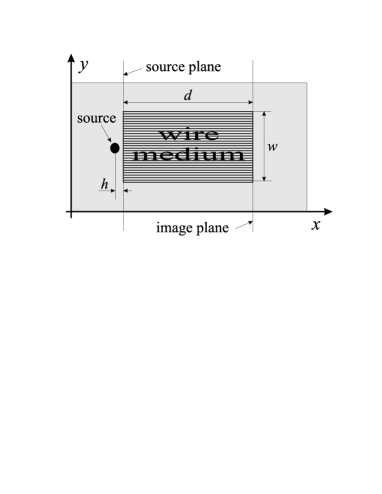
Fig. 2: The layout of the computation domain for two-dimensional FDTD simulations

The polarization is transverse magnetic (TM) with respect to the orientation of the wires (or transverse electric (TE) with respect to the computation domain): The electric field is in the $x-y$ plane and the magnetic field is along $z$-axis. The wire medium has a rectangular shape with dimensions $d\times w$ in $x-y$ plane (see Fig. 2). The wires are oriented along $x$-axis. The wave number corresponding to the plasma frequency of the wire medium is chosen to be four times larger than the wave number of the free space ($k_{p}=4k$). The thickness of the slab $d$ has to be an integer number of half-wavelengths in order to implement the canalization regime [3, 5]. A point magnetic source radiating sinusoidal signal with free space wavelength $\lambda$ is placed at the distance $d$ from the front interface of the wire medium slab. As illustrated in Fig. 2, the front interface of the imaging device is treated as the source plane, and the back interface as the image plane, respectively.

4.1 Transient wave propagation

In the first simulation, see Fig. 3, we have placed the point source in the close vicinity from the front interface of

Fig. 3: Animation: Transient propagation of the wave excited by a point sinusoidal magnetic source located at the $\lambda/200$ distance from the front interface of $1\lambda\times 2\lambda$ slab of the wire medium. Figure: Snapshots of magnetic field $H_{z}$ at the different time steps: (a) $t=175\Delta_{t}$, (b) $t=400\Delta_{t}$, (c) $t=530\Delta_{t}$.

the wire medium slab ($h=\lambda/200$). Such a geometry allows us to illustrate the fact that the waves in the wire medium travel in the fixed direction (along the wires) with the speed of light, in contrast to the free space case where the waves travel with the speed of light in arbitrary direction. The point source creates a cylindrical wavefront in the free space (see Fig. 3) since the waves are allowed to travel in all directions with the same speed. However, as soon as the cylindrical wave enters the wire medium, the form of wavefront changes dramatically (see Fig. 3): the wavefront becomes conical. The waves travel with speed of light along the surface of the wire medium in the free space and excites transmission line modes of the wire medium which travel in the orthogonal direction (along the wires) with the same speed, that is why the form of the wavefront happens to be conical. Note that the front part of the cone contains sub-wavelength information of the source and as soon as the cone reaches the back interface of the slab one can state that the sub-wavelength image is formed. Thus, we conclude that the formation of images happens with the speed of light and all spatial harmonics from the spectrum of the source reaches the image plane at the same time. This fact illustrates the advantage of the canalization principle of sub-wavelength imaging over the regime based on negative refraction and amplification of evanescent waves, where the pumping of the growing evanescent waves takes very long and the sub-wavelength information corresponding to the different spatial harmonics appears at the image plane with significant delay.

4.2 Power flow

In the second simulation, we have placed a point magnetic source at the $\lambda/10$ distance from the $0.5\lambda\times 1\lambda$ slab of wire medium. The power flow diagram in the steady-state regime for this case is presented in Fig. 4.

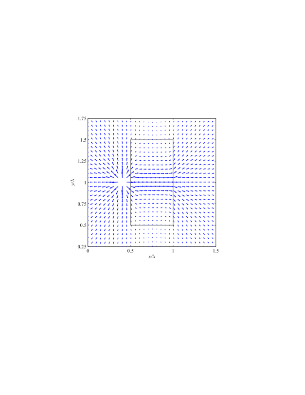
Fig. 4: Power flow diagram in the steady state for the $0.5\lambda\times 1\lambda$ slab of the wire medium excited by a point magnetic source located at the $\lambda/10$ distance from the front interface.

One can see that in the close vicinity of the interfaces the power flow changes direction because of the evanescent extraordinary modes of the wire medium and inside the wire medium the energy transfer happens only along direction of wires with the help of transmission line modes. Also, it is noteworthy that no harmful diffractions from the corners of the slab are observed. This can be explained by the fact that the waves in the wire medium travel and transfer energy only along $x$-axis and no waves travel along $y$-axis. That is why the interfaces in $y$-direction does not reflect any waves and no diffractions from the corners are visible. Due to the absence of diffraction effects it is not mandatory to have the transverse size $w$ of the slab to be significantly larger than the wavelength in order to provide functionality of the transmission device, in contrast to the case of conventional lenses. The transverse dimensions of the transmission device can be practically arbitrary. For example, in the present paper we use one- and two-wavelength wide slabs which demonstrate good sub-wavelength imaging performance.

4.3 Distributions of electric and magnetic fields

In the next simulation, see Fig. 5, we have kept $\lambda/2$ thickness of the slab and $\lambda/10$ distance between source and the wire medium slab, but increased transverse size of the slab up to $2\lambda$. Fig. 5 shows the distributions of electric and magnetic fields after the steady state is reached. The absolute values of these fields are presented in Fig. 6.

Fig. 5: Animation: Distributions of electric and magnetic fields for a $0.5\lambda\times 2\lambda$ slab of the wire medium excited by a point source located at $\lambda/10$ distance from the front interface.

Fig. 6: Absolute values of the fields plotted in Fig. 5

One can see from Fig. 5.a that the non-zero $x$-component of electrical field is present inside the wire medium slab only in the close vicinity of the interfaces. This can be easily explained since only the extraordinary modes of the wire medium have non-zero electric field along the wires, but these modes in the present case are evanescent and decay with distance. That is why the $x$-component of electrical field vanishes in the center of the slab. Inside the wire medium slab, only transmission line modes are present and thus, the electric and magnetic fields have only $y$- and $z$-components, respectively, see Figs. 5.b and 5.c. In accordance to the canalization principle, the transmission line modes deliver images from the front interface to the back one. This is why the absolute values of the fields are the same at the front and back interfaces, see Fig. 6. However, the fields in the image plane appear in out of phase with respect to the fields in the source plane since the thickness of the slab is $\lambda/2$.

4.4 Effect of the slab thickness

The images produced by transmission devices operating in the canalization regime exactly repeat the source distributions if the thickness of the structure is equal to even number of half-wavelengths and appear out of phase if the thickness is equal to odd number of half-wavelengths [3]. In order to demonstrate the case when the image appears in phase with the source we have chosen a wire medium slab with the dimension of $2\lambda\times 1\lambda$. Other parameters are the same as in the previous case.

Fig. 7: Distributions of electric and magnetic fields for a $2\lambda\times\lambda$ slab of the wire medium excited by a point source located at $\lambda/10$ distance from the front interface.

Figs. 7.a, b and c show the distributions of electric and magnetic field in the simulation domain for this case and it is clearly seen that the fields at the back interface of the slab are the same as at the front interface. Additionally, the distribution of magnetic field in the plane $y=\lambda$ is plotted in Fig. 7.d in order to demonstrate that the field inside of the wire medium has harmonic dependence with the period $\lambda$ along the direction of wires. Using this illustration and the fact of magnetic field continuity at the interface between free space and the wire medium, it becomes possible to explain the canalization principle for sub-wavelength imaging: The field at the back interface of the slab repeats the distribution at the front interface because the total thickness of the slab is equal to integer numbers of half-wavelength and at such a distance any harmonic dependence with period $\lambda$ repeats its initial absolute value.

5 Effects of spatial dispersion in modeling of the wire medium

The wire medium is a unique artificial material which possesses strong spatial dispersion effects. It is quite hard to compare properties of this material with media without spatial dispersion, however it is possible to reveal certain similarities and differences. For example, if the spatial dispersion effects are neglected in (1) then one deals with uniaxial Drude material with permittivity tensor

$$\overline{\overline{\varepsilon}}=\varepsilon(\omega){\bf x}{\bf x}+{\bf y}{\bf y}+{\bf z}{\bf z},\qquad\varepsilon(\omega)=1-\frac{k_{p}^{2}}{k^{2}}.$$ (14)

Such a model can be treated as an old and incorrect description of the wire medium [9, 10, 11]. We have replaced the wire medium in simulations corresponding to Fig. 5 by a local uniaxial Drude material with permittivity tensor (14). All other parameters of the structure ($k_{p}=4k$, $h=\lambda/10$, $w=2\lambda$, $d=\lambda/2$, see Fig. 2) were kept unchanged. The FDTD simulation was performed using the updating equation (13). The distributions of the fields in the steady-state regime are presented in Fig. 8.

Fig. 8: Distributions of electric and magnetic field in the steady state for a $0.5\lambda\times 2\lambda$ slab of the uniaxial Drude material (14) with $k_{p}/k=4$ excited by a point source located at $\lambda/10$ distance from the front interface.

One can readily notice strong differences between this figure and Fig. 5 corresponding to the case of the wire medium: The waves inside of the uniaxial Drude material travel not precisely along the anisotropy axis, and thus, they suffer numerous reflections from the edges and corners of the slab. The interference pattern caused by the multiple-reflected waves distorts field distributions in both source and image planes, see Fig. 10.b. This example shows that it is extremely important to take into account the spatial dispersion in modeling of the wire media.

Actually, the wire medium behaves similar to the uniaxial material with permittivity tensor

$$\overline{\overline{\epsilon}}=\infty{\bf x}{\bf x}+{\bf y}{\bf y}+{\bf z}{\bf z}.$$ (15)

This can be explained by the fact that the component $\epsilon(\omega,q_{x})$ of the permittivity tensor of wire medium (1) happens to be infinite for transmission line modes with $q_{x}=\pm k$. We have performed FDTD simulation for the structure as in Fig. 5, but instead of wire medium we used the uniaxial material with infinite permittivity along the anisotropy axis (15). The updating equation for $E_{x}$ component inside such a material is very simple: $E_{x}|^{n+1}_{m_{x},m_{y},m_{z}}=0$. The results of the simulation are presented in Fig. 9.

Fig. 9: Distributions of electric and magnetic fields in the steady state for a slab of the uniaxial material with infinite permittivity along anisotropy axis (15) excited by a point source located at $\lambda/10$ distance from the front interface.

It first appears that Figs. 9 and 5 seem to be identical. However, more precise comparison immediately reveals significant differences: in the case of the uniaxial material with infinite permittivity along anisotropy axis, $x$-component of electric field is zero everywhere inside this material, but in the case of wire medium there are regions near the front and back interfaces of the slab where this component is non-zero. In other words, the model (15) allows to describe transmission line modes of the wire medium, but it does not take into account extraordinary modes of the wire medium. The presence of extraordinary modes in the wire medium makes distributions of the fields in the source and image plane slightly different from those in the case of the uniaxial material with infinite permittivity along the anisotropy axis, see Fig. 10.a.

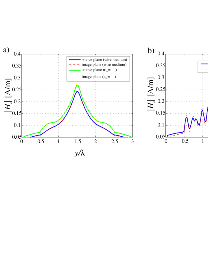
Fig. 10: Absolute values of magnetic field in the source and image planes of the transmission devices formed by three different materials: a) wire medium (Fig. 6), uniaxial material with infinite permittivity along anisotropy axis (Fig. 9); b) uniaxial Drude material (Fig. 8).

The distributions of magnetic field in the source and image planes for the simulations considered in this section are plotted in Fig. 10 for comparison. The slabs of wire medium and uniaxial material with infinite permittivity along the anisotropy axis demonstrate nearly perfect imaging: The distributions of the field in the source and image planes are practically identical. The difference between the distributions can be explained by the fact that high-order spatial harmonics experience non-zero reflections from the wire medium slab as it is shown in [22]. In the case of local uniaxial Drude material, see Fig. 10, these reflections are significantly higher, and strong ripples caused by interference of the waves reflected from the edges and corners of the slab encumber proper imaging operation of the device.

6 Sub-wavelength imaging by the wire medium slabs

In previous sections we have shown good imaging performance of the wire medium slabs. However, we were not able to demonstrate the sub-wavelength imaging capability of such devices since the point source excitations were used in simulations. In order to investigate such capability, we have performed additional simulations with more complicated (sub-wavelength) sources. We have placed three equally spaced magnetic point sources at $\lambda/20$ distance from the front interface of a $0.5\lambda\times 2\lambda$ slab of wire medium. The distance between sources is $\lambda/20$ and the central source is excited in out of phase with respect to the neighboring sources. The proposed three-source configuration creates distribution with two strong maxima at the front interface of the wire medium slab and the distance between these maxima is about $\lambda/10$, see Fig. 11.

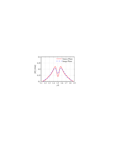
Fig. 11: Absolute values of magnetic field at the source and image planes for a $0.5\lambda\times 2\lambda$ slab of the wire medium excited by three equally spaced magnetic sources with the phase differences equal to $180^{\circ}$ located at $\lambda/20$ distance from the front interface.

Fig. 12: Animation: Distributions of electric and magnetic fields in the steady state for a $0.5\lambda\times 2\lambda$ slab of the wire medium excited by three equally spaced magnetic sources with the phase differences equal to $180^{\circ}$ located at $\lambda/20$ distance from the front interface.

Fig. 13: Absolute values of the fields plotted in Fig. 12.

Results of the spatially dispersive FDTD simulation for excitation of the wire medium slab by the proposed complicated source are presented in Fig. 12. The size of the computation domain, ratio between plasma frequency and operating frequency, FDTD cell size and time step remain the same as in previous sections. The distribution of magnetic field in the image plane is presented in Fig. 11. The two maxima located at $\lambda/10$ distance from each other are clearly resolved by the device, that confirms the sub-wavelength imaging capability of the wire medium lenses. For more details about resolution of such imaging devices see theoretical investigations in [22].

7 Conclusion

The spatially dispersive FDTD method has been developed for efficient modeling of the wave propagation in the wire medium using the effective medium approach. The auxiliary differential equation method is used in order to take into account both the spatial and frequency dispersion of the wire medium. The flat sub-wavelength lenses formed by the wire medium are chosen for the validation of developed spatially dispersive FDTD formulations. Numerical simulations verify the sub-wavelength imaging capability of these structures. The results confirm that the slabs of the wire medium operate in the canalization regime as transmission devices and demonstrate that this regime is not sensitive to the transverse dimensions of these structures.