Photodetachment of H^- by a Short Laser Pulse in Crossed Static Electric and Magnetic Fields

Abstract

(Submitted to Physical Review A)

We present a detailed quantum mechanical treatment of the photodetachment of H^- by a short laser pulse in the presence of crossed static electric and magnetic fields. An exact analytic formula is presented for the final state electron wave function (describing an electron in both static electric and magnetic fields and a short laser pulse of arbitrary intensity). In the limit of a weak laser pulse, final state electron wave packet motion is examined and related to the closed classical electron orbits in crossed static fields predicted by Peters and Delos [Phys. Rev. A 47, 3020 (1993)]. Owing to these closed orbit trajectories, we show that the detachment probability can be modulated, depending on the time delay between two laser pulses and their relative phase, thereby providing a means to partially control the photodetachment process. In the limit of a long, weak pulse (i.e., a monochromatic radiation field) our results reduce to those of others; however, for this case we analyze the photodetachment cross section numerically over a much larger range of electron kinetic energy (i.e., up to 500 cm^-1) than in previous studies and relate the detailed structures both analytically and numerically to the above-mentioned, closed classical periodic orbits.

I Introduction

High resolution studies of atomic Rydberg states in the presence of external static electric and magnetic fields have proved to be exceedingly fruitful for the investigation of atomic dynamics because, owing to the large radial extent and weak binding of atomic Rydberg levels, the effects of external static fields are much more significant for Rydberg levels than for atomic ground or low-lying excited states Braun1993 . Consequently for more than a quarter century (up to the present) experimentalists and theorists have been investigating atomic Rydberg spectra in external fields, including in particular the interesting case of crossed static electric and magnetic fields Braun1993 ; Crosswhite1979 ; Gay1979 ; Korevaar1983 ; Clark83 ; Clark1985 ; Nessmann1987 ; Fauth1987 ; Hare1988 ; Wieb89 ; Gay1989 ; Vincke1992 ; Yeaz93 ; Dippel1994 ; Uzer1994 ; Uzer1996 ; Connerade1997 ; Neum97 ; Uzer1997a ; Uzer1997b ; Taylor1997 ; Sadovskii1998 ; Wunner1998 ; Cederbaum1999 ; Cushman1999 ; Cushman2000 ; Delos2001 ; Uzer2001 ; Schmelcher2001 ; Taylor2002a ; Freu02 ; Taylor2002b ; Valent2003 ; Wunner2003 ; Abdu04 ; Conn05 . These latter investigations for the crossed field case include studies of motional Stark effects on Rydberg atom spectra in a magnetic field Crosswhite1979 , of novel, highly excited resonance states Gay1979 ; Clark1985 ; Nessmann1987 ; Fauth1987 ; Wieb89 ; Vincke1992 ; Dippel1994 ; Connerade1997 ; Cederbaum1999 , of circular Rydberg states Hare1988 , of Rydberg wave packets in crossed fields Gay1989 ; Yeaz93 , of non-hydrogenic signatures in Rydberg spectra Taylor1997 ; Wunner1998 , of doubly-excited states in crossed fields Schmelcher2001 , of recurrence spectra Taylor2002a ; Freu02 ; Taylor2002b , and of various aspects of electron dynamics in combined Coulomb and crossed static electric and magnetic fields Braun1993 ; Uzer1994 ; Uzer1996 ; Neum97 ; Uzer1997a ; Uzer1997b ; Sadovskii1998 ; Cushman1999 ; Cushman2000 ; Delos2001 ; Uzer2001 ; Valent2003 ; Wunner2003 ; Abdu04 ; Conn05 .

The related problem of photodetachment of a weakly bound electron (e.g., as in photodetachment of a negative ion) in the presence of crossed static electric and magnetic fields has been the subject of fewer investigations despite its having a comparably rich spectrum. (Note that the weakly bound electron in a negative ion can simply decay, or become detached, solely due to the presence of the external static electric and magnetic fields, a process that has long been studied theoretically, as in, e.g., Drukarev1972 ; Popov1998 .) Experimentally, crossed field effects have been found to be significant in photodetachment of negative ions in the presence of a static magnetic field owing to the influence of the motional electric field experienced by the detached electron Blumberg1979 ; Yuki97 . The photodetachment spectrum of H^- in the presence of crossed static electric and magnetic fields has been treated theoretically by Fabrikant Fabr91 and by Peters and Delos Peter93 ; Peter93b ; a generalization to the case of photodetachment of H^- in the presence of static electric and magnetic fields of arbitrary orientation has been given by Liu et al. Liu96 ; Liu97 ; Liu97a . In each of these works the static fields are assumed to be sufficiently weak that they do not affect the relatively compact initial state. Fabrikant Fabr91 gave the first quantum treatment of single photon detachment in crossed static electric and magnetic fields using the zero-range potential model to describe the initial state of H^-; rescattering of the electron from the potential was also investigated, although the effect was found to be small except for high magnetic field strengths. Peters and Delos Peter93 gave a semiclassical analysis of H^- photodetachment in crossed fields and correlated significant features of the spectrum with closed classical orbits. Subsequently they derived quantum formulas for this process (using the zero-range potential model for the initial state) and exhibited the connection to their predicted classical closed periodic orbits Peter93b . The generalization of Liu et al. Liu96 ; Liu97 ; Liu97a to the case of static electric and magnetic fields of arbitrary orientation is also based upon the zero-range potential model. In all of these works the electromagnetic field that causes photodetachment is assumed to be weak and monochromatic. Also, the photodetachment spectrum is analyzed numerically only over a very small energy range above threshold.

In this paper we consider detachment of H^- by a short laser pulse in the presence of crossed static electric and magnetic fields. We present an analytic expression for the final state of the detached electron taking into account exactly the effects of the laser field as well as both static fields. The initial state is described by the solution of the zero-range potential, as in all other quantum treatments to date Fabr91 ; Peter93b ; Liu96 ; Liu97 ; Liu97a . We present also an analytic expression for the photodetachment transition amplitude that can be used to describe the probabilities of multiphoton detachment in crossed fields. In this paper, however, our focus is on single photon detachment by short laser pulses and on the connection between the detached electron wave packet motion and the predicted classical closed periodic orbits of Peters and Delos Peter93 . As noted by Alber and Zoller Alber1991 (in connection with electronic wave packets in Rydberg atoms), such wave packets “provide a bridge between quantum mechanics and the classical concept of the trajectory of a particle” and “the evolution of these wave packets provides real-time observations of atomic or molecular dynamics.” We show this connection for the case of short pulse laser-detached electron wave packets in crossed static electric and magnetic fields. In addition, we show analytically how our short pulse results reduce to the quantum monochromatic field results of Fabrikant Fabr91 and Peters and Delos Peter93b in the long pulse limit as well as the connection between our analytic quantum formulation for the photodetachment spectrum and those features that we associate with the predicted classical closed orbits Peter93 . Finally, we present numerical results in the long pulse limit over a large energy range above the single photon detachment threshold in order to demonstrate clearly these manifestations of classical behavior in our predicted photodetachment spectrum.

This paper is organized as follows: In Sec. II we present our theoretical formulation for detachment of H^- by a short laser pulse in the presence of crossed static electric and magnetic fields. In particular, in this section (with details given in an Appendix) we present an exact, analytic expression for the wave function for an electron interacting with both the laser pulse and the crossed static electric and magnetic fields. We present here also analytic expressions for the transition probability amplitudes for both a single laser pulse and a double laser pulse (i.e., two coherent single pulses separated by a time delay). In addition, the long pulse (monochromatic field) limit of our results is presented and this result is compared with a number of prior works for various static field cases. In Sec. III we establish the connection between the long pulse limit of our results and the closed classical periodic orbits predicted by Peters and Delos Peter93 . In Sec. IV we present our numerical results, starting first with a comparison with prior results for the long pulse (monochromatic field) case and then examining the short pulse case, including the final state motion of the detached electron wave packets.

II Theoretical Formulation

We consider photodetachment of H^- by one or more short laser pulses in the presence of crossed static electric and magnetic fields. In the final state, we assume the detached electron experiences only the laser and static fields; we ignore final state interaction of the electron with the residual hydrogen atom. For weak external fields, this is expected to be a good approximation for this predominantly single photon process. In this section, we first give the $S$-matrix transition amplitude for photodetachment of H^-. Then we present an exact quantum mechanical solution to the time-dependent Schrödinger equation for the final state of the detached electron in both the crossed static electric and magnetic fields and the time dependent laser pulse. We then use this result together with S-matrix theory to obtain detachment rates and cross sections. Atomic units are used throughout this paper unless otherwise stated.

II.1 $S$-matrix Transition Amplitude for Photodetachment of H^-

We adopt the Keldysh approximation for the final-state, i.e., we neglect the binding potential Reiss80 . In this case, the $S$-matrix transition amplitude from the initial state $\psi_{i}$ to the final state $\psi_{f}$ is given by

$$S_{fi}=-i\int_{-\infty}^{\infty}dt^{\prime}\left\langle\psi_{f}(\mathbf{p},t^{\prime})|V_{I}(t^{\prime})|\psi_{i}(\mathbf{p},t^{\prime})\right\rangle,$$ (1)

where $V_{I}$ represents the laser-electron interaction and the bracket $\left\langle{}\right\rangle$ stands for integration over momentum space. For the zero range potential for which the bound state wave function has the form $e^{-\kappa r}/r$, the $S$-matrix element in Eq. (1) can be shown to be gauge-invariant Gao90 ; Niki66 . Such a bound state wave function can be used to represent the weakly bound electron of H^-. We use that of Ohmura and Ohmura Ohmu60 , which in momentum space is given by

$$\psi_{i}(\mathbf{p},t)=\frac{C_{i}}{\sqrt{2\pi}}\frac{e^{-i\varepsilon_{i}t}}{p^{2}/2-\varepsilon_{i}},$$ (2)

where $C_{i}$ is a normalization constant and $\varepsilon_{i}$ is the initial state energy. Using the variational results of Ref. Ohmu60 and effective range theory for a weakly bound $s$-electron Beth50 , one obtains Du88 $C_{i}=0.31552$ and $\varepsilon_{i}=-0.027751$ a.u.. The gauge-invariant $S$-matrix transition amplitude for H^- detachment is then given by (cf. Eq. (27) of Ref. Gao90 )

$$\left(S_{fi}\right)_{k_{x}k_{y}n_{z}}=i\int_{-\infty}^{\infty}dt^{\prime}\left\langle\psi_{f}(\mathbf{p},t^{\prime})|C_{i}/\sqrt{2\pi}\right\rangle e^{-i\varepsilon_{i}t^{\prime}}.$$ (3)

II.2 The Final State Wave Function

Figure 1: Geometrical arrangement of fields in photodetachment of $H^{-}$ by a linearly polarized laser (with electric field $\bf{E_{L}}$) in the presence of crossed static electric ($\bf{E_{S}}$) and magnetic ($\bf{B}$) fields. Both the laser and the static electric fields point along the $z$-axis. As indicated, the drift motion of the detached electron is along the $y$-axis.

In order to calculate the $S$-matrix transition amplitude in Eq. (3), we present in this section an analytical expression for the final state wave function $\psi_{f}$. As aforementioned, we neglect the binding potential after detachment. Therefore, $\psi_{f}$ is actually a Volkov-type wave function that describes a free electron moving in the combined field of the crossed static electric and magnetic fields and the time-dependent electric field associated with the short laser pulse. In Fig. 1 we illustrate the configuration of the external fields in which the detached electron moves: the uniform static magnetic field defines the $x$ axis and the static electric field defines the $z$ axis, i.e.,

$$\mathbf{B}=B\hat{\mathbf{i}}$$ (4)

$$\mathbf{E_{S}}=E_{S}\hat{\mathbf{k}}.$$ (5)

We assume that each laser pulse has the following general form,

$$\mathbf{E_{L}}(t)=E_{0}e^{-\alpha^{2}\left(t-\tau\right)^{2}}\sin\left(\omega t+\beta\right)\hat{\mathbf{k}},$$ (6)

where $\omega$ is the laser frequency, $\tau$ is the time delay with respect to $t=0$, and $\beta$ is a (generally constant) phase. The duration of the laser pulse is defined to be the full width at half maximum (FWHM) of the laser intensity, and is given by

$$T_{p}=\sqrt{2\ln 2}/\alpha.$$ (7)

We introduce the vector potentials for the magnetic field and the laser field respectively, as follows:

$$\mathbf{A_{B}}=-zB\hat{\mathbf{j}},$$ (8)

$$\mathbf{A_{L}}(t)=-c\int_{-\infty}^{t}\mathbf{E_{L}}(t^{\prime})dt^{\prime},$$ (9)

where $c$ is the speed of light in vacuum.

The final state wave function for the detached electron is obtained as the solution of the time-dependent Schrödinger equation (TDSE) in momentum space,

$$i\frac{\partial}{\partial t}\psi_{f}^{(p)}(\mathbf{p},t)=H\psi_{f}^{(p)}(\mathbf{p},t),$$ (10)

in which the Hamiltonian $H$ is given by

$$H(\mathbf{p},t) = \frac{1}{2}\left[\mathbf{p}+\frac{1}{c}\left(\mathbf{A}_{L}+\mathbf{A}_{B}\right)\right]^{2}+\mathbf{\hat{r}}\cdot\mathbf{E}_{S}$$ (12)

$$= -\frac{1}{2}\omega_{c}^{2}\frac{\partial^{2}}{\partial p_{z}^{2}}-i\omega_{c}\left(p_{y}-\frac{E_{S}}{\omega_{c}}\right)\frac{\partial}{\partial p_{z}}+\frac{1}{2}p_{z}^{2}+\frac{1}{c}p_{z}A_{L}(t)$$

$$+\frac{1}{2}p_{x}^{2}+\frac{1}{2}p_{y}^{2}+\frac{1}{2c^{2}}A_{L}^{2}(t),$$

where $\omega_{c}=B/c$ is the cyclotron frequency.

It can be shown that Eq. (10) has an exact analytical solution. The details of the derivation are presented in Appendix A. The final expression of the solution is given by

$$\psi_{f}^{(p)}(\mathbf{p},t) = \delta(p_{x}-k_{x})\delta(p_{y}-k_{y})\exp\left[-i\varepsilon_{f}t-if(t)\right]$$ (13)

$$\times \omega_{c}^{-1/4}g_{n_{z}}\left(\sqrt{2}\zeta_{p_{z}}\right)\exp\left[-ib(k_{y},t)\sqrt{2}\zeta_{p_{z}}\right],$$

in which $g_{n_{z}}\left(x\right)$ is defined by

$$g_{n_{z}}\left(x\right)=\frac{1}{\sqrt{2^{n_{z}}n_{z}!\sqrt{\pi}}}e^{-x^{2}/2}H_{n_{z}}(x),$$ (14)

where $H_{n_{z}}(x)$ is the $n_{z}\it{th}$ Hermite polynomial. In Eq. (13) we have also defined

$$\varepsilon_{f}=\frac{1}{2}\left(k_{x}^{2}+k_{y}^{2}\right)+\varepsilon_{n_{z}}-\frac{1}{2}\omega_{c}\zeta_{k_{y}}^{2},$$

$$\hskip 13.6572pt=\frac{1}{2}k_{x}^{2}+\frac{E_{S}}{\sqrt{\omega_{c}}}\zeta_{k_{y}}+\varepsilon_{n_{z}}+\frac{1}{2}\frac{E_{S}^{2}}{\omega_{c}^{2}},$$ (15)

$$f(t)=\frac{1}{\sqrt{\omega_{c}}}\zeta_{k_{y}}\xi(t)+\frac{1}{2c^{2}}\int_{-\infty}^{t}A_{L}^{2}(t^{\prime})dt^{\prime}-\int_{-\infty}^{t}L(t^{\prime})dt^{\prime},$$ (16)

$$b(k_{y},t)=\zeta_{k_{y}}-\dot{\xi}(t)/\sqrt{\omega_{c}^{3}},$$ (17)

where the arguments $\zeta_{p_{z}}$ and $\zeta_{k_{y}}$ are given by

$$\zeta_{p_{z}}(t)=\left[p_{z}-\xi(t)\right]/\sqrt{2\omega_{c}},$$ (18)

$$\zeta_{k_{y}}=\frac{1}{\sqrt{\omega_{c}}}\left(k_{y}-\frac{E_{S}}{\omega_{c}}\right),$$ (19)

and the energy of the $n_{z}th$ Landau level $\varepsilon_{n_{z}}$ in Eq. (15) is given by

$$\varepsilon_{n_{z}}=\left(n_{z}+\frac{1}{2}\right)\omega_{c}.$$ (20)

In Eq. (16), $L(t)$ and $\xi(t)$ are functions related to the vector potential of the short laser pulse. $L(t)$ is defined as

$$L(t)=\frac{1}{2\omega_{c}^{2}}\dot{\xi}^{2}(t)-\frac{1}{2}\xi^{2}(t)-\frac{1}{c}A_{L}(t)\xi(t),$$ (21)

while $\xi(t)$ satisfies the following differential equation:

$$\ddot{\xi}(t)+\omega_{c}^{2}\xi(t)=-\frac{\omega_{c}^{2}}{c}A_{L}(t),$$ (22)

where $\ddot{\xi}(t)$ denotes the second derivative of $\xi(t)$. We present the exact solution for $\xi(t)$ in Appendix B. However, in the long pulse case ($\alpha/\omega\ll 1$), a simplified expression for $\xi(t)$ can be obtained as

$$\xi(t)\simeq a\left(\omega\right)e^{-\alpha^{2}(t-\tau)^{2}}\cos\left(\omega t+\beta\right),$$ (23)

where we have defined

$$a\left(\omega\right)=\frac{E_{0}\,\omega_{c}^{2}}{\omega\left(\omega^{2}-\omega_{c}^{2}\right)}.$$ (24)

In this case, the first derivative, $\dot{\xi}(t)$, is thus given by

$$\dot{\xi}(t)\simeq-\omega a\left(\omega\right)e^{-\alpha^{2}(t-\tau)^{2}}\sin\left(\omega t+\beta\right).$$ (25)

In order to investigate wave packet dynamics, it is useful to derive an expression for the final state wave function in which its $z$ component is given in coordinate space. This is achieved by taking the Fourier transform of Eq. (13) with respect to $p_{z}$, i.e.,

$$\psi_{f}^{(z)}(p_{x},p_{y},z,t)\equiv\psi_{k_{x},k_{y},n_{z}}^{(z)}(p_{x},p_{y},z,t)=\frac{1}{\sqrt{2\pi}}\int_{-\infty}^{\infty}dp_{z}\psi_{f}^{(p)}(\mathbf{p},t)e^{izp_{z}}.$$ (26)

Changing the integration variable to $\zeta_{p_{z}}$ (cf. Eq. (18)), we obtain

$$\psi_{f}^{(z)}(p_{x},p_{y},z,t) = \delta(p_{x}-k_{x})\delta(p_{y}-k_{y})i^{n_{z}}\omega_{c}^{1/4}g_{n_{z}}\left[\sqrt{\omega_{c}}z-b(k_{y},t)\right]$$ (27)

$$\times\exp\left[iz\xi(t)-i\varepsilon_{f}t-if(t)\right],$$

where we have made use of Eqs. 7.388(2) and 7.388(4) in Ref. Gradsh .

II.3 $S$-matrix Amplitude for Photodetachment of H^-

In order to examine the motion of the detached electron wave packet in crossed $\mathbf{E}$ and $\mathbf{B}$ fields, we define in analogy to Eq. (23) of Ref. Wang95 a time-dependent transition amplitude $R_{fi}(t)$ from the initial state to the final state $(k_{x},k_{y},n_{z})$:

$$\left(R_{fi}(t)\right)_{k_{x}k_{y}n_{z}} = i\frac{C_{i}}{\sqrt{2\pi}}\sqrt{2\omega_{c}}\int_{-\infty}^{t}dt^{\prime}e^{i\varepsilon_{fi}t^{\prime}+if(t^{\prime})}$$ (28)

$$\times\int_{-\infty}^{\infty}\omega_{c}^{-1/4}g_{n_{z}}\left(\sqrt{2}\zeta_{p_{z}}\right)\exp\left[ib(k_{y},t^{\prime})\sqrt{2}\zeta_{p_{z}}\right]d\zeta_{p_{z}},$$

where $\varepsilon_{fi}=\varepsilon_{f}-\varepsilon_{i}$, $b(k_{y},t^{\prime})$ is given by Eq. (17), and where we have used Eq. (13) for the final state wave function in Eq. (3). Using Eqs. 7.388(2) and 7.388(4) in Ref. Gradsh to carry out the integration over $\zeta_{p_{z}}$, we obtain

$$\left(R_{fi}(t)\right)_{k_{x}k_{y}n_{z}}=i^{n_{z}+1}C_{i}\int_{-\infty}^{t}dt^{\prime}e^{i\varepsilon_{fi}t^{\prime}+if(t^{\prime})}\omega_{c}^{1/4}g_{n_{z}}\left[b(k_{y},t^{\prime})\right].$$ (29)

Note that in the limit of $t\rightarrow\infty$, $R_{fi}(t)$ reduces to the $S$-matrix transition amplitude (3), i.e.:

$$\left(S_{fi}\right)_{k_{x}k_{y}n_{z}}=\lim_{t\rightarrow\infty}\left(R_{fi}(t)\right)_{k_{x}k_{y}n_{z}}.$$ (30)

In principle, with this analytical $S$-matrix amplitude one can readily calculate the total and multiphoton transition rates, as done for H^- detachment in a static electric field in Ref. Gao90 . However, in the present paper, we restrict our consideration to the one-photon detachment process (Note that there are still many cycles in the laser pulses that we will consider in this work). Our analytical results facilitate easy comparison with some other previous results. Consequently, we evaluate Eq. (29) only to first order in the laser electric field strength $E_{0}$, i.e., we employ the following approximations:

$$e^{if(t^{\prime})} \simeq 1+if(t^{\prime})$$

$$\simeq 1+i\frac{1}{\sqrt{\omega_{c}}}\zeta_{k_{y}}\xi(t^{\prime}),$$

$$g_{n_{z}}\left[b(k_{y},t^{\prime}\right]\simeq g_{n_{z}}(\zeta_{k_{y}})+g_{n_{z}}^{\prime}(\zeta_{k_{y}})\left[-\frac{\dot{\xi}(t^{\prime})}{\sqrt{\omega_{c}^{3}}}\right],$$

where $g_{n_{z}}^{\prime}(\zeta_{k_{y}})$ stands for the derivative of $g_{n_{z}}(\zeta_{k_{y}})$. Thus, to first order in $E_{0}$, the time-dependent transition amplitude is given by

$$\left(R_{fi}^{(1)}(t)\right)_{k_{x}k_{y}n_{z}} = i^{n_{z}+1}C_{i}\omega_{c}^{1/4}g_{n_{z}}(\zeta_{k_{y}})\int_{-\infty}^{t}dt^{\prime}e^{i\varepsilon_{fi}t^{\prime}}$$ (31)

$$-i^{n_{z}+1}C_{i}\omega_{c}^{1/4}g_{n_{z}}^{\prime}(\zeta_{k_{y}})\int_{-\infty}^{t}dt^{\prime}e^{i\varepsilon_{fi}t^{\prime}}\frac{\dot{\xi}(t^{\prime})}{\sqrt{\omega_{c}^{3}}}$$

$$-i^{n_{z}}C_{i}\zeta_{k_{y}}\omega_{c}^{1/4}g_{n_{z}}(\zeta_{k_{y}})\int_{-\infty}^{t}dt^{\prime}e^{i\varepsilon_{fi}t^{\prime}}\frac{\xi(t^{\prime})}{\sqrt{\omega_{c}}}.$$

Note that, as usual, the first term in Eq. (31) does not contribute to the photodetachment process (since for $t\rightarrow\infty$, the only contributions are for $\varepsilon_{fi}\rightarrow 0$); hence this term is discarded in the following discussion.

In the long pulse approximation, with the help of Eqs. (23) and (25), one can show that

$$\left(R_{fi}^{(1)}(t)\right)_{k_{x}k_{y}n_{z}} = i^{n_{z}+1}C_{i}g_{n_{z}}^{\prime}(\zeta_{k_{y}})\frac{\omega a(\omega)}{\omega_{c}^{5/4}}\int_{-\infty}^{t}dt^{\prime}e^{-\alpha^{2}(t^{\prime}-\tau)^{2}+i\varepsilon_{fi}t^{\prime}}\sin\left(\omega t^{\prime}+\beta\right)$$ (32)

$$-i^{n_{z}}C_{i}\zeta_{y}g_{n_{z}}(\zeta_{k_{y}})\frac{(\omega)}{\omega_{c}^{1/4}}\int_{-\infty}^{t}dt^{\prime}e^{-\alpha^{2}(t^{\prime}-\tau)^{2}+i\varepsilon_{fi}t^{\prime}}\cos\left(\omega t^{\prime}+\beta\right),$$

which reduces to

$$\left(R_{fi}^{(1)}(t)\right)_{k_{x}k_{y}n_{z}} = -i^{n_{z}}C_{i}\frac{a(\omega)}{2\omega_{c}^{5/4}}\left[\omega g_{n_{z}}^{\prime}(\zeta_{k_{y}})+\omega_{c}\zeta_{y}g_{n_{z}}(\zeta_{k_{y}})\right]$$ (33)

$$\times\int_{-\infty}^{t}dt^{\prime}e^{-\alpha^{2}(t^{\prime}-\tau)^{2}+i\varepsilon_{fi}t^{\prime}-i\omega t^{\prime}-i\beta}$$

if we neglect the emission process (i.e., if we discard terms involving $e^{+i\omega t^{\prime}}$).

The integration over $t^{\prime}$ in Eq. (33) can be carried out analytically:

$$\int_{-\infty}^{t}dt^{\prime}e^{-\alpha^{2}(t^{\prime}-\tau)^{2}+i\varepsilon_{fi}t^{\prime}-i\omega t^{\prime}-i\beta}$$

$$= \frac{\sqrt{\pi}}{2\alpha}\left\{\mathop{\rm erf}\left[\alpha\left(t-\tau\right)-i\frac{\varepsilon_{fi}-\omega}{2\alpha}\right]+1\right\}$$

$$\times\exp\left[-\frac{\left(\varepsilon_{fi}-\omega\right)^{2}}{4\alpha^{2}}+i\left(\varepsilon_{fi}-\omega\right)\tau-i\beta\right].$$

Thus, for the single laser pulse in Eq. (6), the first-order time-dependent transition amplitude in the long pulse approximation is given by

$$\left(R_{fi}^{(1)}(t)\right)_{k_{x}k_{y}n_{z}}^{\text{sgl}} = -i^{n_{z}}C_{i}\frac{\pi a(\omega)}{2\omega_{c}^{5/4}}\left[\omega g_{n_{z}}^{\prime}(\zeta_{k_{y}})+\omega_{c}\zeta_{y}g_{n_{z}}(\zeta_{k_{y}})\right]$$ (34)

$$\times D_{\text{sgl}}(\varepsilon_{fi},t)\delta_{\alpha}(\varepsilon_{fi}-\omega),$$

where we have defined

$$D_{\text{sgl}}(\varepsilon_{fi},t)=e^{i\left(\varepsilon_{fi}-\omega\right)\tau-i\beta}\left[1+\mathop{\rm erf}\left[\alpha\left(t-\tau\right)-i\frac{\varepsilon_{fi}-\omega}{2\alpha}\right]\right],$$ (35)

and have also introduced the quasi-$\delta$-function Wang95 ,

$$\delta_{\alpha}(\varepsilon_{fi}-\omega)=\left(2\pi^{1/2}\alpha\right)^{-1}\exp\left[-\frac{\left(\varepsilon_{fi}-\omega\right)^{2}}{4\alpha^{2}}\right].$$ (36)

In the limit that our finite laser pulse becomes a monochromatic plane wave, the quasi-$\delta$-function becomes the usual Dirac $\delta$-function,

$$\delta(\varepsilon_{fi}-\omega)=\lim_{\alpha\rightarrow 0}\delta_{\alpha}(\varepsilon_{fi}-\omega).$$ (37)

Taking the limit $t\rightarrow+\infty$, we obtain from Eq. (34) the following analytical expression for the $S$-matrix amplitude for the case of a single, finite laser pulse:

$$\left(S_{fi}^{(1)}\right)_{k_{x}k_{y}n_{z}}^{\text{sgl}} = -i^{n_{z}}C_{i}\frac{\pi a(\omega)}{\omega_{c}^{5/4}}\left[\omega g_{n_{z}}^{\prime}(\zeta_{k_{y}})+\omega_{c}\zeta_{y}g_{n_{z}}(\zeta_{k_{y}})\right]$$ (38)

$$\times e^{i\left(\varepsilon_{fi}-\omega\right)\tau-i\beta}\delta_{\alpha}(\varepsilon_{fi}-\omega),$$

where we have used the fact that $\mathop{\rm erf}(\infty+iy)=1$ for any finite real number $y$.

II.4 Detached Electron Wave Packet

We may obtain the detached electron wave packet probability amplitude as a sum over all final states of the product of the time-dependent transition amplitude for transition to the final state $(k_{x},k_{y},n_{z})$ at a particular time $t$ [Eq. (34)] and the wave function [Eq. (27)] for that state (cf. Sec. II. D of Ref. Wang95 ):

$$\psi_{\text{WP}}(p_{x},p_{y},z,t)=\sum_{n_{z}=0}^{\infty}\int_{-\infty}^{\infty}dk_{x}\int_{-\infty}^{\infty}dk_{y}\psi_{k_{x},k_{y},n_{z}}^{(z)}(p_{x},p_{y},z,t)\left(R_{fi}^{(1)}(t)\right)_{k_{x}k_{y}n_{z}}.$$ (39)

By using Eqs. (27) and (34), the wave packet for the single laser pulse (6) is given by

$$\psi^{\text{sgl}}_{\text{WP}}(p_{x},p_{y},z,t) = -C_{i}\frac{\pi a(\omega)}{2\omega_{c}}\sum_{n_{z}=0}^{\infty}\left(-1\right)^{n_{z}}\exp\left[iz\xi-i\varepsilon_{f}^{\prime}t-i\frac{1}{\sqrt{\omega_{c}}}\zeta_{p_{y}}\xi\right]$$ (40)

$$\times g_{n_{z}}\left[\sqrt{\omega_{c}}z-b(p_{y},t)\right]\left[\omega g_{n_{z}}^{\prime}(\zeta_{p_{y}})+\omega_{c}\zeta_{y}g_{n_{z}}(\zeta_{p_{y}})\right]$$

$$\times D_{\text{sgl}}(\varepsilon_{fi}^{\prime},t)\delta_{\alpha}(\varepsilon_{fi}^{\prime}-\omega)$$

where $\zeta_{p_{y}}$ and $b(p_{y},t)$ are defined by Eqs. (19) and (17) respectively, $\varepsilon_{fi}^{\prime}=\varepsilon_{f}^{\prime}-\varepsilon_{i}$, and $\varepsilon_{f}^{\prime}$ is given by Eq. (15) with $\zeta_{k_{y}}$ replaced by $\zeta_{p_{y}}$.

II.5 $S$-matrix and Wave Packet Amplitudes for the Double Pulse Case

We consider here the case that there are two laser pulses of the form of Eq. (6), with the second one delayed with respect to the first by a time interval $\tau$ and having a relative phase of $\beta$, i.e.,

$$\mathbf{E}_{\mathbf{L}}^{\mathbf{{dbl}}}(t)=E_{0}\left[e^{-\alpha^{2}t^{2}}\sin\left(\omega t\right)+e^{-\alpha^{2}\left(t-\tau\right)^{2}}\sin\left(\omega t+\beta\right)\right]\hat{\mathbf{k}}.$$ (41)

To first order in $E_{0}$, it is easy to show that for the double laser pulse case, the time-dependent transition amplitude is given by

$$\left(R_{fi}^{(1)}(t)\right)_{k_{x}k_{y}n_{z}}^{\text{dbl}} = -i^{n_{z}}C_{i}\frac{\pi a(\omega)}{2\omega_{c}^{5/4}}\left[\omega g_{n_{z}}^{\prime}(\zeta_{k_{y}})+\omega_{c}\zeta_{y}g_{n_{z}}(\zeta_{k_{y}})\right]$$ (42)

$$\times D_{\text{dbl}}(\varepsilon_{fi},t)\delta_{\alpha}\left(\varepsilon_{fi}-\omega\right),$$

where the function $D_{\text{dbl}}(\varepsilon_{fi},t)$ is given by

$$D_{\text{dbl}}(\varepsilon_{fi},t)=1+\mathop{\rm erf}\left[\alpha t-i\frac{\varepsilon_{fi}-\omega}{2\alpha}\right]+e^{i\left(\varepsilon_{fi}-\omega\right)\tau-i\beta}\left\{1+\mathop{\rm erf}\left[\alpha\left(t-\tau\right)-i\frac{\varepsilon_{fi}-\omega}{2\alpha}\right]\right\}.$$ (43)

When $t\rightarrow\infty$, the above formula reduces to

$$\left(S_{fi}^{(1)}\right)_{k_{x}k_{y}n_{z}}^{\text{dbl}} = \lim_{t\rightarrow\infty}\left(R_{fi}^{(1)}(t)\right)_{k_{x}k_{y}n_{z}}^{\text{dbl}}$$ (44)

$$= -i^{n_{z}}C_{i}\frac{\pi a(\omega)}{\omega_{c}^{5/4}}\left[\omega g_{n_{z}}^{\prime}(\zeta_{k_{y}})+\omega_{c}\zeta_{y}g_{n_{z}}(\zeta_{k_{y}})\right]$$

$$\times\left[1+e^{i\left(\varepsilon_{fi}-\omega\right)\tau-i\beta}\right]\delta_{\alpha}\left(\varepsilon_{fi}-\omega\right).$$

The wave packet amplitude for the double laser pulse case is correspondingly given by

$$\psi_{\text{WP}}^{\text{dbl}}(p_{x},p_{y},z,t) = -C_{i}\frac{\pi a(\omega)}{2\omega_{c}}\sum_{n_{z}=0}^{\infty}\left(-1\right)^{n_{z}}\exp\left[iz\xi-i\varepsilon_{f}^{\prime}t-i\frac{1}{\sqrt{\omega_{c}}}\zeta_{p_{y}}\xi\right]$$ (45)

$$\times g_{n_{z}}\left[\sqrt{\omega_{c}}z-b(p_{y},t)\right]\left[\omega g_{n_{z}}^{\prime}(\zeta_{p_{y}})+\omega_{c}\zeta_{y}g_{n_{z}}(\zeta_{p_{y}})\right]$$

$$\times D_{\text{dbl}}(\varepsilon_{fi}^{\prime},t)\delta_{\alpha}\left(\varepsilon_{fi}^{\prime}-\omega\right).$$

II.6 Photodetachment Cross Section

The transition probability to a particular final state $\left(k_{x},k_{y},n_{z}\right)$ is given by

$$P_{k_{x}k_{y}n_{z}}=\left|\left(S_{fi}\right)_{k_{x}k_{y}n_{z}}\right|^{2},$$ (46)

and the total photodetachment probability is calculated by integrating over all final states,

$$P=\sum\limits_{n_{z}=0}^{\infty}\int_{-\infty}^{\infty}dk_{x}\int_{-\infty}^{\infty}dk_{y}P_{k_{x}k_{y}n_{z}}.$$ (47)

For an infinitely long, monochromatic beam, the probability $P$ is proportional to time, $t$. In this case, it does not make sense to talk about the total transition probability. Instead, one normally considers the total transition rate, $W$, which is given by Reiss80

$$W=\lim_{t\rightarrow\infty}\frac{1}{t}P.$$ (48)

The total photodetachment cross section is obtained by dividing the total photodetachment rate $W$ by the photon flux $F$ (the number of photons per unit area per unit time):

$$\sigma_{pw}=\frac{W}{F},$$ (49)

where ‘pw’ stands for the monochromatic plane wave case.

For the short laser pulse case, it does not make sense to talk about a transition rate since the transition probability is not simply proportional to time $t$. In addition, the photon flux $F$ is not well defined. Nevertheless, it is possible to renormalize the total probability for detachment by a short laser pulse in such a way that the renormalized probability reduces, in the limit of an infinitely long pulse, to the usual formula for the photodetachment cross section. Since the renormalized probability will have the dimensions of area, we denote it as an effective photodetachment cross section, $\sigma$. To derive this effective cross section, one uses the time duration of the laser pulse as the unit of time. One calculates the total photodetachment probability $P$ during the laser pulse duration and the total number of photons per unit area (i.e., the photon density), $\Sigma$, during the laser pulse duration. Then an effective photodetachment cross section, $\sigma$, may be defined as

$$\sigma=\frac{P}{\Sigma}.$$ (50)

Clearly $\sigma$ defined in this way has the dimensions of a cross section. In the rest of this paper, $\sigma$ should be understood to be this effective photodetachment cross section, i.e., calculated according to Eq. (50). We shall show below that this $\sigma$ for the short laser pulse case reduces in the limit $\alpha\rightarrow 0$ (cf. Eq. (6)) to the usual photodetachment cross section for a monochromatic plane wave.

It has been shown by Wang and Starace Wang95 that for a single Gaussian pulse defined by Eq. (6) with $\tau=\beta=0$, the photon density $\Sigma$ is given by the following formula:

$$\Sigma_{\text{sgl}}=\frac{cE_{0}^{2}}{8\pi\omega}\frac{\sqrt{2\pi}}{2\alpha}.$$ (51)

For the double pulse case (cf. Eq. (41)), $\Sigma$ is correspondingly given by

$$\Sigma_{\text{dbl}}=\frac{cE_{0}^{2}}{8\pi\omega}\frac{\sqrt{2\pi}}{\alpha}\left[1+\cos\beta\exp(-\alpha^{2}\tau^{2}/2)\right].$$ (52)

Taking $\beta$ and $\tau$ to be zero in Eq. (38), and using Eqs. (24) and (46)-(51), we have for the photodetachment cross section of H^- by a single pulse of the form of Eq. (6):

$$\sigma^{(1)} = \frac{4\pi^{2}C_{i}^{2}\omega_{c}^{2}}{c\omega(\omega^{2}-\omega_{c}^{2})^{2}}\sum\limits_{n_{z}=0}^{\infty}\int_{-\infty}^{\infty}d\zeta_{k_{y}}\left[\zeta_{k_{y}}\omega_{c}g_{n_{z}}\left(\zeta_{k_{y}}\right)+\omega g_{n_{z}}^{\prime}\left(\zeta_{k_{y}}\right)\right]^{2}$$ (53)

$$\times\int_{-\infty}^{\infty}dk_{x}\overline{\delta}_{\alpha}\left(\varepsilon_{fi}-\omega\right),$$

where we have employed a second quasi-$\delta$ function Wang95 ,

$$\overline{\delta}_{\alpha}\left(\varepsilon_{fi}-\omega\right)=\frac{1}{\alpha\sqrt{2\pi}}\exp\left[-\frac{\left(\varepsilon_{fi}-\omega\right)^{2}}{2\alpha^{2}}\right],$$ (54)

which reduces to the usual Dirac $\delta$-function in the limit of a monochromatic plane wave, i.e.,

$$\delta\left(\varepsilon_{fi}-\omega\right)=\lim_{\alpha\rightarrow 0}\overline{\delta}_{\alpha}\left(\varepsilon_{fi}-\omega\right).$$ (55)

Note that

$$\varepsilon_{fi}-\omega=\frac{1}{2}\left[k_{x}^{2}+Q\left(\zeta_{k_{y}}\right)\right],$$ (56)

in which we have defined (cf. Eq. 15)

$$Q\left(\zeta_{k_{y}}\right)=\frac{2E_{S}}{\sqrt{\omega_{c}}}\left(\zeta_{k_{y}}+\zeta_{\min}\right),$$ (57)

where

$$\zeta_{\min}=\frac{\sqrt{\omega_{c}}}{E_{S}}\left[(n_{z}+\frac{1}{2})\omega_{c}+\frac{E_{S}^{2}}{2\omega_{c}^{2}}-\varepsilon_{i}-\omega\right].$$ (58)

The integration over $k_{x}$ in Eq. (53) has an analytical result when $Q\left(\zeta_{k_{y}}\right)\geq 0$. The result is

$$\int_{-\infty}^{\infty}dk_{x}\frac{1}{\sqrt{2\alpha^{2}\pi}}\exp\left[-\frac{\left(\varepsilon_{fi}-\omega\right)^{2}}{2\alpha^{2}}\right]$$

$$= \frac{1}{\sqrt{2\alpha^{2}\pi}}\int_{-\infty}^{\infty}dk_{x}\exp\left[-\frac{\left(k_{x}^{2}+Q\left(\zeta_{k_{y}}\right)\right)^{2}}{8\alpha^{2}}\right]$$

$$= \frac{1}{\alpha\sqrt{2\pi}}\sqrt{\frac{E_{S}}{\sqrt{\omega_{c}}}\left(\zeta_{k_{y}}+\zeta_{\min}\right)}\exp\left[-\frac{E_{S}^{2}\left(\zeta_{k_{y}}+\zeta_{\min}\right)^{2}}{4\omega_{c}\alpha^{2}}\right]K_{\frac{1}{4}}\left[\frac{E_{S}^{2}\left(\zeta_{k_{y}}+\zeta_{\min}\right)^{2}}{4\omega_{c}\alpha^{2}}\right]$$

where we have used the following formula (cf. Eq. (3.323) on p.307 of Ref. Gradsh ):

$$\int_{0}^{\infty}dx\exp\left[-\beta^{2}x^{4}-2\gamma^{2}x^{2}\right]=2^{-3/2}\frac{\gamma}{\beta}e^{\gamma^{4}/2\beta^{2}}K_{\frac{1}{4}}\left(\gamma^{4}/2\beta^{2}\right),$$

which holds for $\left|\arg\beta\right|<\frac{\pi}{4}$ and $\left|\arg\gamma\right|<\frac{\pi}{4}$, and where $K_{\nu}(z)$ is a modified Bessel function (cf. p.375 of Ref. Abra65 ). When $Q\left(\zeta_{k_{y}}\right)<0$, the integration in Eq. (II.6) must be done numerically.

II.6.1 Plane Wave Limit of the Cross Section

In the plane wave limit, $\alpha\rightarrow 0$, the integration over $k_{x}$ (making use of Eq. (54)) becomes

$$\int_{-\infty}^{\infty}dk_{x}\delta\left(\varepsilon_{fi}-\omega\right)=\int_{-\infty}^{\infty}dk_{x}\delta\left(\frac{1}{2}k_{x}^{2}+\frac{1}{2}Q\left(\zeta_{k_{y}}\right)\right).$$ (60)

This integral is non-zero only when $\varepsilon_{fi}-\omega=\frac{1}{2}k_{x}^{2}+\frac{1}{2}Q\left(\zeta_{k_{y}}\right)=0$, i.e., when we have strict energy conservation. For non-zero real $k_{x}$, we should thus require

$$Q\left(\zeta_{k_{y}}\right)=\frac{2E_{S}}{\sqrt{\omega_{c}}}\left(\zeta_{k_{y}}+\zeta_{\min}\right)<0$$

or

$$\tilde{\zeta}_{k_{y}}\equiv-\zeta_{k_{y}}>\zeta_{\min}.$$ (61)

Thus we have that

$$\int_{-\infty}^{\infty}dk_{x}\delta\left(\frac{1}{2}k_{x}^{2}+\frac{1}{2}Q\left(\zeta_{k_{y}}\right)\right)$$

$$= \frac{1}{|Q|^{1/2}}\int_{-\infty}^{\infty}dk_{x}\left[\delta\left(k_{x}+|Q|^{1/2}\right)+\delta\left(k_{x}-|Q|^{1/2}\right)\right]$$

$$= \frac{2\omega_{c}^{1/4}}{\sqrt{2E_{S}}}\frac{1}{\sqrt{-\zeta_{k_{y}}-\zeta_{\min}}},$$

In the plane wave limit, we have then (converting $\zeta_{k_{y}}$ to $\tilde{\zeta}_{k_{y}}$)

$$\sigma_{\alpha=0}^{(1)}=\frac{8\pi^{2}C_{i}^{2}\omega_{c}^{9/4}}{c\omega(\omega^{2}-\omega_{c}^{2})^{2}}\frac{1}{\sqrt{2E_{S}}}\sum\limits_{n_{z}=0}^{\infty}\int_{\zeta_{\min}}^{\infty}\frac{d\tilde{\zeta}_{k_{y}}}{\sqrt{\tilde{\zeta}_{k_{y}}-\zeta_{\min}}}\left[\tilde{\zeta}_{k_{y}}\omega_{c}g_{n_{z}}\left(\tilde{\zeta}_{k_{y}}\right)+\omega g_{n_{z}}^{\prime}\left(\tilde{\zeta}_{k_{y}}\right)\right]^{2}.$$ (62)

We consider now two limiting cases, corresponding to weak static magnetic and electric fields respectively.

The weak magnetic field limit.

The plane wave cross section in Eq. (62) can be simplified when the cyclotron frequency, $\omega_{c}$, is much smaller than the laser frequency, $\omega$, i.e., $\omega_{c}\ll\omega$. In this case,

$$\sigma_{\alpha=0,\omega_{c}\ll\omega}^{(1)}=\frac{3\sigma^{0}}{k^{3}}\frac{\omega_{c}^{9/4}}{\sqrt{2E_{S}}}\sum\limits_{n_{z}=0}^{\infty}\int_{\zeta_{\min}}^{\infty}d\tilde{\zeta}_{k_{y}}\frac{g_{n_{z}}^{\prime 2}\left(\tilde{\zeta}_{k_{y}}\right)}{\sqrt{\tilde{\zeta}_{k_{y}}-\zeta_{\min}}},$$ (63)

where we have defined

$$\sigma^{0}=\frac{8\pi^{2}C_{i}^{2}}{3c\omega^{3}}k^{3},$$ (64)

in which $\sigma^{0}$ is the photodetachment cross section for H^- in the monochromatic field limit in the absence of any static fields, and $k$ is the magnitude of the detached electron’s momentum, $k^{2}=2E_{f}=2\left(\omega+\varepsilon_{i}\right)$.

We note that our weak magnetic field result in Eq. (63) agrees with the formula of Peters and Delos (see Eqs. (3.6) and (3.7a) of Ref. Peter93b ). Eq. (63) agrees also with Fabrikant’s result (see Eq. (53) of Ref. Fabr91 ) except for the extra term in his formula that accounts for final-state interaction of the electron with the atomic residue.

Weak static electric field limit.

In the limit $E_{S}\rightarrow 0$, we have that $\ \zeta_{\min}\rightarrow-\infty$. And we have also

$$\lim_{E_{S}\rightarrow 0}\sqrt{2E_{S}}\sqrt{\tilde{\zeta}_{k_{y}}-\zeta_{\min}}=\omega_{c}^{1/4}\sqrt{2\omega_{c}\left[\left(\varepsilon_{i}+\omega\right)/\omega_{c}-(n_{z}+\frac{1}{2})\right]}.$$ (65)

Substituting this result into Eq. (62) and carrying out the integration involving the Hermite polynomials, we obtain

$$\sigma_{\alpha=0,E_{S}=0}^{(1)}=\frac{8\pi^{2}C_{i}^{2}\omega_{c}^{2}}{c\omega(\omega+\omega_{c})^{2}}\sum\limits_{n_{z}=0}^{n_{1}}\left[\frac{\omega^{2}+\omega_{c}^{2}}{(\omega-\omega_{c})^{2}}n_{z}+\frac{1}{2}\right]\frac{1}{\sqrt{2\omega_{c}\left[\left(\varepsilon_{i}+\omega\right)/\omega_{c}-(n_{z}+\frac{1}{2})\right]}}$$ (66)

where the upper limit of summation, $n_{1}$, is the largest integer that satisfies,

$$n_{1}<\left[\frac{\varepsilon_{i}+\omega}{\omega_{c}}-\frac{1}{2}\right].$$

Eq. (66) is exactly the same as Gao’s result for the one-photon detachment cross section in a static uniform magnetic field (see Eq. (31) of Ref. Gao90a ).

II.6.2 Cross Section for the Double Pulse Case

From Eqs. (44),  (47), (50) and (52), it is easy to show that for the double laser pulse case, the cross section is given by

$$\sigma_{\text{dbl}}^{(1)} = \frac{4\pi^{2}C_{i}^{2}\omega_{c}^{2}}{c\omega(\omega^{2}-\omega_{c}^{2})^{2}}\sum\limits_{n_{z}=0}^{\infty}\int_{-\infty}^{\infty}d\zeta_{k_{y}}\left[\zeta_{y}\omega_{c}g_{n_{z}}\left(\zeta_{k_{y}}\right)+\omega g_{n_{z}}^{\prime}\left(\zeta_{k_{y}}\right)\right]^{2}$$ (67)

$$\times\int_{-\infty}^{\infty}dk_{x}\frac{1+\cos\left[\left(\varepsilon_{fi}-\omega\right)\tau-\beta\right]}{1+\cos\beta\exp(-\alpha^{2}\tau^{2}/2)}\overline{\delta}_{\alpha}\left(\varepsilon_{fi}-\omega\right).$$

We note that for $\tau=\beta=0$, this formula reduces to the single pulse result in Eq. (53), as it should (cf. Eq. (41)).

III Connections to Classical Closed Orbits

In the previous section we have derived a general quantum mechanical expression for the (effective) photodetachment cross section for H^- by a short laser pulse in the presence of crossed static electric and magnetic fields. We have also shown that our plane wave limit result (given by Eq. (62)) reduces for the limiting cases of weak static magnetic (cf. Eq. (63)) or weak static electric (cf. Eq. (66)) fields to known results of others. Magnetic field strengths, $B$, that are readily available at present in the laboratory are weak in the sense that they satisfy the relation, $\omega_{c}\ll\omega$. Therefore the quantum result for the photodetachment cross section in the plane wave limit given in Eq. (63) is of great interest owing to the possibility of experimental measurements with currently available technology. In this section we analyze this equation for the purpose of making connection with the classical closed orbits analyzed by Peters and Delos Peter93 . This connection will prove useful for interpreting some of the numerical predictions presented in the next section.

For $\omega\gg\omega_{c}$, the detached electron energy lies in the region of large $n_{z}$. In this limit the integrand in Eq. (63) becomes highly oscillatory, as may be seen by considering the large $n_{z}$ (Plancherel-Rotach) limit of the Hermite function, $g_{n_{z}}$ Szego39 :

$$g_{n_{z}}(\tilde{\zeta}_{k_{y}})\simeq\sqrt{\frac{2}{\pi\sqrt{2n_{z}(1-\eta^{2})}}}\left\{\sin\left[\left(n_{z}+\frac{1}{2}\right)\left(\eta\sqrt{1-\eta^{2}}-\arccos\eta\right)+\frac{3\pi}{4}\right]+O(n_{z}^{-1})\right\},$$ (68)

where we have defined

$$\eta\equiv\tilde{\zeta}_{k_{y}}/\sqrt{2n_{z}+1},$$ (69)

and note that

$$\epsilon\leqslant\arccos\eta\leqslant\pi-\epsilon,\text{}\epsilon\rightarrow 0^{+},$$

i.e., the argument of the Hermite function, $g_{n_{z}}(\tilde{\zeta}_{k_{y}})$, must lie between the classical turning points:

$$-\sqrt{2n_{z}+1}<\tilde{\zeta}_{k_{y}}<\sqrt{2n_{z}+1}.$$

The function $g_{n_{z}}^{\prime}\left(\tilde{\zeta}_{k_{y}}\right)$ that occurs in the integrand of Eq. (63) may be calculated by differentiation of Eq. (68) with respect to $\tilde{\zeta}_{k_{y}}$, as follows:

$$g_{n_{z}}^{\prime}\left(\tilde{\zeta}_{k_{y}}\right) = \frac{\partial\eta}{\partial\tilde{\zeta}_{k_{y}}}\frac{\partial}{\partial\eta}g_{n_{z}}\left(\tilde{\zeta}_{k_{y}}\right)=\frac{1}{\sqrt{2n_{z}+1}}\sqrt{\frac{2}{\pi\sqrt{2n_{z}}}}$$ (70)

$$\times \left\{\frac{\eta}{2}\left(1-\eta^{2}\right)^{-\frac{5}{4}}\sin\left[S(n_{z},\eta)\right]+(2n_{z}+1)\left(1-\eta^{2}\right)^{\frac{1}{4}}\cos\left[S(n_{z},\eta)\right]\right\},$$

where we have defined the phase

$$S(n_{z},\eta)=\left(n_{z}+\frac{1}{2}\right)\left(\eta\sqrt{1-\eta^{2}}-\arccos\eta\right)+\frac{3\pi}{4}.$$ (71)

Assuming that $n_{z}\gg 1$, Eq. (70) can be simplified (in particular, the first term within the curly brackets can be ignored in comparison with the second term), so that we obtain:

$$g_{n_{z}}^{\prime}\left(\tilde{\zeta}_{k_{y}}\right)\simeq\sqrt{\frac{2}{\pi}}(2n_{z})^{\frac{1}{4}}(1-\eta^{2})^{\frac{1}{4}}\cos\left[S(n_{z},\eta)\right].$$ (72)

Owing to the fact that $n_{z}$ is large, the phase function $S(n_{z},\eta)$ changes significantly as $\eta$ varies (cf. Eq. (71)), so that $g_{n_{z}}^{\prime}\left(\tilde{\zeta}_{k_{y}}\right)$ oscillates rapidly as a function of $\tilde{\zeta}_{k_{y}}$. From Eq. (63) we see that the magnitude of the photodetachment cross section will have the highest maxima when the squares of the various $g_{n_{z}}^{\prime}\left(\tilde{\zeta}_{k_{y}}\right)$ functions that are summed (over $n_{z}$) have their maxima and minima in phase with each other, i.e., when neighboring phase functions differ by an integer multiple of $\pi$:

$$S\left(n_{z},\eta(n_{z})\right)-S\left(n_{z}-1,\eta(n_{z}-1)\right)\simeq\frac{d}{dn_{z}}S(n_{z},\eta)=j\pi\text{, where }j=0,\pm 1,\pm 2,...$$

This condition is similar to that found for the largest local maxima in the photodetachment cross section of $H^{-}$ in the presence of parallel static electric and magnetic fields Wang97 . We compute the total derivative of $S(n_{z},\eta)$ as:

$$\frac{d}{dn_{z}}S(n_{z},\eta)=\frac{\partial S}{\partial n_{z}}+\frac{\partial S}{\partial\eta}\frac{\partial\eta}{\partial n_{z}}$$ (73)

The partial derivatives of the phase $S(n_{z},\eta)$ follow straightforwardly from the definition in Eq. (71). The partial derivative, ${\partial\eta}/{\partial n_{z}}$, is calculated using the definition in Eq. (69) and the expression for $\tilde{\zeta}_{k_{y}}$ obtained from the energy conservation condition, $\varepsilon_{fi}-\omega=0$, together with Eqs. (56)-(58) and Eq. (61). After some straightforward algebra, one obtains:

$$\frac{d}{dn_{z}}S(n_{z},\eta)=-\arccos\eta+\sqrt{1-\eta^{2}}\frac{\omega_{c}}{E_{S}}\sqrt{2\varepsilon_{n_{z}}}=j\pi.$$ (74)

The condition (74) for the highest local maxima in the photodetachment cross section (63) may be re-written in terms of the scaled energy $\varepsilon$, defined by

$$\varepsilon=\varepsilon_{n_{z}}\left(\frac{\omega_{c}}{E_{S}}\right)^{2},$$ (75)

and the angle $\varphi$, defined by

$$\varphi=\frac{\pi}{2}-\arccos\eta,$$ (76)

to obtain:

$$\cos\varphi+\frac{\varphi}{\sqrt{2\varepsilon}}-\frac{1}{\sqrt{2\varepsilon}}\left(j+\frac{1}{2}\right)\pi=0.$$ (77)

This result is identical to the classical equation expressing the relationship of the azimuthal angle $\varphi$ and the scaled energy $\varepsilon$ for a closed orbit of an electron in crossed fields (see Eq. (3.12) of Ref. Peter93 ).

The classical Hamiltonian corresponding to the quantum Hamiltonian (12) for the detached electron is given by

$$H_{\text{cls}} = \frac{1}{2}\omega_{c}^{2}z^{2}+\omega_{c}z\left(p_{y}-\frac{E_{S}}{\omega_{c}}\right)+\frac{1}{2}p_{z}^{2}+\frac{1}{2}p_{x}^{2}+\frac{1}{2}p_{y}^{2}$$ (78)

$$= \frac{1}{2}p_{x}^{2}+\frac{E_{S}}{\omega_{c}}p_{y}+\frac{1}{2}p_{z}^{2}+\frac{1}{2}\left[\omega_{c}z+\left(p_{y}-\frac{E_{S}}{\omega_{c}}\right)\right]^{2}-\frac{1}{2}\frac{E_{S}^{2}}{\omega_{c}^{2}}.$$

Denoting

$$\varepsilon_{z}=\frac{1}{2}p_{z}^{2}+\frac{1}{2}\left[\omega_{c}z+\left(p_{y}-\frac{E_{S}}{\omega_{c}}\right)\right]^{2},$$ (79)

and introducing the following scaled coordinate, momentum, and time variables,

$$\tilde{\mathbf{q}}=\frac{\omega_{c}^{2}}{E_{S}}\mathbf{q},$$ (80)

$$\tilde{\mathbf{p}}=\frac{\omega_{c}}{E_{S}}\mathbf{p},$$ (81)

$$\tilde{t}=\omega_{c}t,$$ (82)

Eq. (78) may be rewritten as

$$E=\varepsilon+\frac{1}{2}\tilde{p}_{x}^{2}+\tilde{p}_{y}-\frac{1}{2},$$ (83)

where $E=\omega_{c}^{2}(\omega+\varepsilon_{i})/{E_{S}^{2}}$ is the scaled total energy and $\varepsilon$ is given by Eq. (75) in which the quantum energy $\varepsilon_{n_{z}}$ (cf. Eq. (20)) is replaced by the classical energy $\varepsilon_{z}$ in Eq. (79).

With the help of Eqs. (20), (19) and (61), it is easy to show from the definition (69) that

$$\eta=-\frac{p_{y}-E_{S}/\omega_{c}}{\sqrt{2\varepsilon_{n_{z}}}},$$ (84)

which can be rewritten, in terms of scaled energies, as

$$\eta=\frac{\varepsilon-(E-1/2)}{\sqrt{2\varepsilon}},$$ (85)

by using the energy conservation equation (83) and the fact that $p_{x}=0$ for closed orbits. Substituting Eq. (85) into Eq. (76), we can rewrite Eq. (77) as

$$\Lambda(\varepsilon)\equiv\sqrt{2\varepsilon-\left[\varepsilon-(E-1/2)\right]^{2}}-\arccos\left[\frac{\varepsilon-(E-1/2)}{\sqrt{2\varepsilon}}\right]=j\pi.$$ (86)

For a given scaled total energy $E$, the number of the solutions of Eq. (86) gives the total number of closed orbits. The return time of a closed orbit in crossed fields is given by Peter93

$$T_{\text{ret}}=2(\omega_{c})^{-1}\sqrt{2\varepsilon}\cos\varphi,$$ (87)

which can be rewritten with the help of Eqs. (76) and (85) as

$$T_{\text{ret}}=2(\omega_{c})^{-1}\sqrt{2\varepsilon-\left[\varepsilon-(E-1/2)\right]^{2}}.$$ (88)

As discussed in Peter93 , there exists a very important group of closed orbits whose total energies are given approximately (in the large energy limit) by

$$E_{j}^{b}\simeq\frac{\pi^{2}}{2}\frac{E_{S}^{2}}{\omega_{c}^{2}}\left[\left(j+\frac{1}{2}\right)^{2}-\frac{3}{\pi^{2}}\right],$$ (89)

where $j=1,2,3,...$. These are called boundary energies, because for each $j$ a new closed orbit appears at the energy given by Eq. (89) and for higher total energies this newborn closed orbit will split (or “bifurcate”) into a pair of closed orbits with two different energies and return times, given by Eqs. (86) and (88).

Actually, each boundary energy defines the onset of large oscillations in the cross section. However, the largest amplitude oscillation in the cross section occurs at a slightly higher energy at which a different type of closed orbit occurs that has a truly circular motion in the drift frame in the $y$-$z$ plane. The energy of this orbit may be obtained by setting the initial momentum along the $y$ axis equal to the drift velocity, i.e.,

$$p_{y}^{0}=\frac{E_{S}}{\omega_{c}}.$$ (90)

From the energy conservation equation (83) and the fact that $p_{x}=0$ for a closed orbit, we have $\varepsilon=E-1/2$. Substituting this result into Eq. (86) gives

$$\sqrt{2\varepsilon}=(j+\frac{1}{2})\pi,$$ (91)

which in unscaled variables corresponds to a total energy equal to

$$\overline{E}_{j}=\frac{\pi^{2}}{2}\frac{E_{S}^{2}}{\omega_{c}^{2}}\left[\left(j+\frac{1}{2}\right)^{2}+\frac{1}{\pi^{2}}\right].$$ (92)

Comparing Eqs. (89) and (92), one sees that the energy difference between the boundary orbits and the orbits having $p_{y}^{0}$ equal to the drift velocity is $2{E_{S}^{2}}/{\omega_{c}^{2}}$, independent of the value of $j$. Boundary closed orbits satisfy $\partial\Lambda(\varepsilon)/\partial\varepsilon=0$, which gives the relationship $\varepsilon=E+\frac{3}{2}$ in the large energy limit. Closed orbits for which Eq. (90) applies have $\varepsilon=E-\frac{1}{2}$. From Eqs. (88) and (91), we find for these latter orbits that

$$T_{\text{ret}}=(j+\frac{1}{2})T_{B},$$ (93)

where $T_{B}={2\pi}/{\omega_{c}}$ is the cyclotron period and $j$ is a positive integer. This formula is very similar to that obtained for the case of parallel static electric and magnetic fields  Pete94 ; Wang97 , in which the largest oscillation amplitude of the cross section corresponds to classical orbits for which for an electron is ejected along the static field direction and reflected by the static electric field such that its return time satisfies $T_{\text{ret}}=jT_{B}$. In the parallel fields case, the motion in the plane perpendicular to the magnetic field is simply cyclotron motion with period $T_{B}$. Classical closed orbits having a return time equal to an integer multiple of $T_{B}$ are associated with the largest oscillations in the cross section Wang97 .

In the crossed fields case, however, the situation is much more complicated. However, since $\varepsilon_{z}$ (cf. Eq. (79)) is conserved, when the detached electron has an initial momentum $p_{y}^{0}$ given by Eq. (90) (and an initial position $z=0$), the initial momentum along the $z$ axis takes its maximum value. This implies that this particular closed orbit starts out (in the drift frame) aligned with the laser polarization direction. These circular orbits (in the drift frame), having energies given by Eq. (92), are associated with the largest amplitude oscillation of the cross section.

IV Results and Discussion

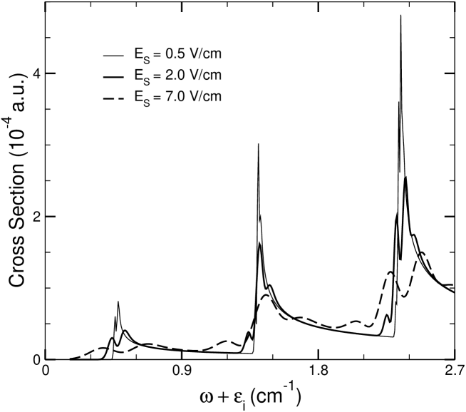
Figure 2: Photodetachment cross section for $H^{-}$ in the plane wave limit for a static magnetic field $B=1$ T and three different values of the static electric field strength. Results are plotted versus detached electron kinetic energy above the zero field detachment threshold, $\omega+\varepsilon_{i}$, up to $2.7$ cm^-1.

In this section we present numerical results based on the quantum mechanical theoretical formulation presented above. We present first plane wave limit results for the photodetachment cross section of $H^{-}$ in the presence of crossed static electric and magnetic fields over a much larger energy range than in prior works Fabr91 ; Peter93 ; Peter93b . This large range allows us to demonstrate very clearly the signatures of the predicted classical closed orbits Peter93 , both in the energy spectrum and in the time (i.e., Fourier transform) spectrum. We examine next the short laser pulse case, demonstrating first the effects of laser pulse duration on the photodetachment cross section. We then examine the detached electron wave packet dynamics in the $y$-$z$ plane and the possibility of modulating the detachment cross section by pump probe (Ramsey interference) techniques. The connection between the time development of the quantum wave packet of the detached electron and the predicted classical closed orbits is also discussed.

IV.1 Photodetachment Cross Section in the Plane Wave Limit

IV.1.1 Static Electric Field Dependence for Near Threshold Energies

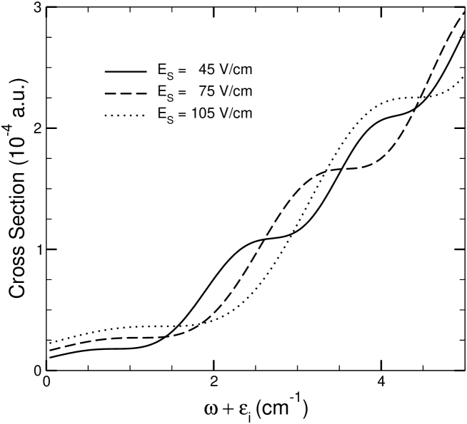
Figure 3: Same as Fig. 2 but for three higher static electric field strengths and detached electron kinetic energies up to $5$ cm^-1.

In Figs. 2 and 3 we present the photodetachment cross section for $H^{-}$ for a static magnetic field, $B=1$ T, and six different values of the static electric field, $E_{S}$. Our quantum theory predictions are obtained from the plane wave limit result given in Eq. (62). One sees in Fig. 2 that, as noted by Fabrikant Fabr91 , even a very small static electric field removes the known singularity in the detachment cross section for energies corresponding to integer multiples of the cyclotron frequency in the pure magnetic field case (see, e.g., Gao90a ). In particular, for $E_{S}=0.5$ V/cm, the behavior of the cross section is very similar to that of the pure magnetic field case Gao90a (to which our results reduce in the limit of zero static electric field, as shown in Sec. II.F.1(b) above), but without the cyclotron singularities. On the other hand, beginning with $E_{S}=7$ V/cm, the oscillatory modulation of the cross section by the static electric field becomes obvious. As shown in Fig. 3 the frequency of this modulation decreases as the static electric field magnitude increases, just as is found for the case of a pure static electric field or for the case of parallel static magnetic and electric fields (see, e.g., Wang95 ). One sees also that the cross section becomes non-zero at the zero-field threshold owing to the lowering of the threshold by the static electric field.

Figure 4: Photodetachment cross section for $H^{-}$ in the plane wave limit for $B=1$ T, $E_{S}=60$ V/cm, and detached electron kinetic energies up to $30$ cm^-1.

For the present crossed static magnetic and electric field case, the modulation of the cross section becomes increasingly complex the higher the maximum total energy $E_{f}$ becomes. For a maximum detached electron kinetic energy of 30 cm^-1, Fig. 4 shows that the oscillatory modulations differ above and below approximately 15 cm^-1. For energies below 15 cm^-1, there exists only a sinusoidal modulation. Above about 15 cm^-1, the modulation consists of more than one frequency and becomes more complicated the higher in energy one looks.

In order to examine these structures in detail, it is instructive to plot only the oscillatory part of the cross section, which is defined by

$$\sigma_{\text{osc}}=\sigma_{\alpha\rightarrow 0}^{(1)}-\sigma^{0},$$ (94)

where $\sigma_{\alpha\rightarrow 0}^{(1)}$ is the total cross section in the plane wave limit (given by Eq. (62)) and $\sigma^{0}$ is the photodetachment cross section in the absence of any external static fields (given by Eq. (64)). Figure 5 shows the oscillatory part of the cross section over three different energy ranges, corresponding to total energies up to 60 cm^-1, 180 cm^-1, and 500 cm^-1 respectively. While the oscillatory modulations of the cross section become increasingly dense and complex as the total energy increases, we see also that clear patterns in the spectra emerge and become more obvious the higher in energy we look. The onset of these repetitive patterns is indicated in each panel by the vertical dotted lines, which represent the locations of the boundary energies Peter93 defined by Eq. (89). The peak amplitudes are indicated by the open triangles at the energies defined by Eq. (92), which correspond to the locations of circular classical orbits in the drift frame. The connection of these classical closed orbits and our quantum mechanical cross sections can be most easily investigated in the time domain, which we consider next.

IV.1.2 Fourier Transform Spectra and Closed Classical Orbits

Figure 5: The oscillatory part of the cross section, $\sigma_{\rm{osc}}$ (cf. Eq. (94)), for $B=1$ T and $E_{S}=60$ V/cm for $\omega+\varepsilon_{i}$ ranging from (a) 0 to 60 cm^-1; (b) 0 to 180 cm^-1; (c) 0 to 500 cm^-1. Dashed lines indicate the boundary energies (cf. Eq. (89)) at which a new closed orbit appears Peter93 and the open triangles indicate the energies at which the amplitude of the oscillatory part of the quantum cross section is expected to have a local maximum (cf. Eq. (92)).

Figure 6: Fourier transform spectra for the oscillatory part of the cross section (cf. Eq. (94)) for different maximum energies, $E_{f}^{max}=\omega+\varepsilon_{i}$, as indicated in each panel. See text for a detailed description.

The Fourier transform of the oscillatory part of the photodetachment cross section, $\sigma_{\text{osc}}$, is presented in Fig. 6 for increasing values of the maximum total detached electron kinetic energy, $E_{f}^{max}$. Times are given in units of the cyclotron period, $T_{B}$. We see from Fig. 6(a) that at the lowest maximum energy, only one peak appears in the time spectrum. The peak position indicates the return time (i.e., orbit period) of a closed classical orbit having an energy of 10.98 cm^-1. As $E_{f}^{max}$ increases to 15.91 cm^-1 in (b), another peak emerges. This corresponds to the first classical boundary energy (cf. Eq. (89)) for $j=1$. Unlike the case of classical dynamics, however, where the boundary energy is sharply defined, our calculations indicate that the second peak in Fig. 6(b) begins to appear around the energy 13.5 cm^-1. Note also that the first peak in (b) shifts to the right as compared to that in (a). This indicates that the return time of the first closed orbit increases when the total energy increases. In panel (c) we observe that the second peak increases in magnitude while the first peak decreases in magnitude. In panel (d), when the total energy equals 21.97 cm^-1, one observes the bifurcation of the second peak that first appeared in panel (b). For $E_{f}^{max}=48.49$ cm^-1, in panel (e), one sees the appearance of a third peak around 2.4 $T_{B}$ and notice that the width of the splitting of the second peak increases as compared to that in (d). The left and right boundaries of the split and broadened second peak correspond to the return times of the two bifurcated orbits at the maximum available total energy $E_{f}^{max}$. The serrated U-shaped region between the left and right boundaries of the split second peak correspond to the return times of the two bifurcated orbits for lower total energies (e.g., such as those two shown in panel (d) for a total energy of 21.97 cm^-1). Finally, in panel (f) for a slightly higher total energy we observe that the third peak grows in magnitude relative to the first and second (split) peaks.

Consider now a much larger total final state energy, $E_{f}^{max}$ = 500 cm^-1. The oscillatory part of the cross section is shown in Fig. 5(c). In this figure, the dashed lines correspond to the seven boundary orbit energies, given by Eq. (89), that appear for energies up to 500 cm^-1, and the triangles correspond to the seven circular orbit (in the drift frame) energies, given by Eq. (92). The Fourier transform spectrum for energies in the range from 0 - 500 cm^-1 is shown in Fig. 7(a), while the Fourier transform of only the part of the spectrum in the range from 400 - 500 cm^-1 is shown in Fig. 7(b). In (a), the open circles denote the return times (periods) of the 15 closed classical orbit solutions of Eq. (86) that exist for a total energy of 500 cm^-1. These periods are calculated using Eq. (88) and the results are given in Table 1 together with the corresponding orbit energies. (Note that for each $j>0$ and for a total energy $E$ not equal to one of the boundary energies given by Eq. (89), Eq. (86) has two solutions.) The open triangles, on the other hand, correspond to the circular orbits in the drift frame corresponding to the local maximum amplitudes of the oscillatory part of the cross section; their return times are given by the very simple Eq. (93).

Table 1: Numerical solutions of Eq. (86) for the energies, $\varepsilon_{j}^{\pm}$(in units of cm^-1), for the closed orbits that exist for a total energy $\omega+\varepsilon_{i}=500$ cm^-1 (302.869 in scaled units) and the corresponding closed orbit periods, $T_{j}^{\pm}$ (in units of $T_{B}$), calculated from Eq. (88). Note that there is only one solution for the case $j=0$.

$j$	0	1	2	3	4	5	6	7
$\varepsilon_{j}^{-}$	461.459	462.389	463.987	466.337	469.595	474.056	480.398	491.231
$T_{j}^{-}$	0.959	1.918	2.876	3.831	4.783	5.730	6.665	7.571
$\varepsilon_{j}^{+}$	—	542.137	541.0371	539.127	536.264	532.160	526.143	515.609
$T_{j}^{+}$	—	1.041	2.082	3.126	4.172	5.224	6.286	7.378

Note that the bowl-like structures appearing in Fig. 7(a) above each open triangle result from the fact that closed orbits have different return times for each different total energy and from the fact that the Fourier transform spectrum in this figure results from a large range of total energies, i.e., from 0 to 500 cm^-1. When we calculate the Fourier transform of the oscillatory part of the cross section over only the limited energy range, $400$ cm^-1 $\leq\omega+\varepsilon_{i}\leq 500$ cm^-1, as in Fig. 7(b), then we observe that the first 13 peaks are approximately located at the positions of the first 13 closed classical orbit periods given in Table 1, which were calculated for a maximum total energy of $500$ cm^-1. The energy region $0\leq\omega+\varepsilon_{i}\leq 400$ cm^-1 is thus inferred to be responsible for the bowl-like structures in Fig. 7(a) owing to the shifts of the lowest 13 classical orbit periods (having $j\leq 6$) for lower total energies. The bowl-like structure remains between the 14th and 15th closed classical orbits (having $j=7$) as this pair of orbits first occurs above a total energy of approximately 455 cm^-1 (cf. Fig. 5(c)). We also observe from the data in Figs. 5 and 7 that the oscillation amplitude of the cross section becomes larger as the total energy increases.

Figure 7: Fourier transform spectra of the oscillatory part of the cross section, $\sigma_{\rm{osc}}$ (cf. Eq. (94)), given in Fig. 5 (c) calculated over two different energy ranges: (a) $0\leq\omega+\varepsilon_{i}\leq 500$ cm^-1; (b) $400$ cm^-1 $\leq\omega+\varepsilon_{i}\leq 500$ cm^-1. In (a) the open circles indicate the return times (i.e., orbit periods) of the 15 closed orbits for $\omega+\varepsilon_{i}=500$ cm^-1 (see Table 1). Also in (a), the open triangles indicate the return times of the circular closed orbits (in the drift frame) having $\tilde{p}_{y}^{0}=1$ (cf. Eqs. (81) and (90)); these return times are given by Eq. (93).

IV.2 Detachment by Short Laser Pulses

Photodetachment by means of one or more short laser pulses differs from that by a monochromatic laser. Most obviously, the pulse bandwidth affects the measured spectrum of detached electrons. In addition, short laser pulses produce localized detached electron wave packets whose motion in crossed fields can be investigated and compared to classical predictions Alber1991 ; Garraway1995 ; Bluhm1996 . Most interesting, perhaps, is the possibility of controlling the modulation of the detachment spectrum by variation of the parameters of one or more laser pulses. In the rest of this section, we examine each of these topics in turn for the crossed static electric and magnetic field case.

We note first, however, several previous works on related problems. Ramsey interference effects resulting from photodetachment of H^- by two short, coherent laser pulses as a function of their relative phase was examined by Wang and Starace for the case of a static electric field Wang93 and the case of parallel static electric and magnetic fields Wang95 . The latter work Wang95 showed that a large modulation of the effective detachment probability can be achieved by optimizing the static field magnitudes and the time delay between laser pulses, as follows: the field magnitudes should be such that the classical time for reflection of an electron back to the origin by the static electric field equals an integer multiple of the harmonic oscillator period for electron motion in the static magnetic field; also, the time delay of the second pulse should coincide with the classical time for the electron’s return to the origin. For the case of a single short laser pulse, Du Du95 examined the photodetachment of H^- in the presence of a static electric field using modified closed orbit formulas. He showed that when the laser pulse duration is shorter than particular closed orbit periods, then those orbits no longer contribute to the photodetachment spectrum. Finally, Zhao et al. Zhao99 have derived a uniform semiclassical formula for the photodetachment cross section of a negative ion by a short laser pulse for the case of parallel static electric and magnetic fields.

Figure 8: Effective photodetachment cross section of H^- (cf. Eq. (53)) by a single laser pulse of the form (6) with four different pulse durations (cf. Eq. (7) in the presence of crossed static electric and magnetic fields, $E_{S}=15$ V/cm and $B=1$ T. Results are plotted vs. electron kinetic energy beginning from the zero-field threshold. Also shown (dotted line) is the photodetachment cross section for the case of a continuous (monochromatic) laser without any external static fields present.

IV.2.1 Pulse Duration Effects

The fundamental difference between using a short laser pulse and using a continuous (monochromatic) laser is the bandwidth of the short laser pulse. In the former case, the laser pulse will excite a group of final states that form an electron wave packet, whereas in the latter case only a well-defined final state will be reached. In our present case of detachment in the presence of crossed static electric and magnetic fields, the spacing of Landau levels is very small (0.93 cm^-1 for $B=1$ T), so that one expects that even a quite long pulse having a duration of several picoseconds will have considerable finite bandwidth effects on the detached electron wave packet and its dynamics.

In Fig. 8, we present the effective total cross section (cf. Eq. (53)) for a laser pulse of the form (6) (with $\tau=\beta=0$) and four different pulse durations (cf. Eq. (7)) in the presence of crossed static electric and magnetic fields of magnitudes $E_{S}=15$ V/cm and $B=1$ T. As we see from Fig. 8, for the longest pulse duration, 240 ps, the effective cross section is identical with that for a (monochromatic) plane wave. As the pulse duration decreases, the modulation of the cross section is suppressed, beginning at the highest energies shown and progressing to structures at lower energies. Thus, when the pulse duration is reduced to 45 ps, the modulation structure beyond the energy 2.3 cm^-1 is largely suppressed. As the pulse duration is further reduced to 30 ps, even the modulation between 1 and 2 cm^-1 decreases in magnitude. At the shortest pulse duration, 15 ps, the oscillatory structure completely disappears and the effective cross section becomes a smooth curve passing through the oscillatory cross sections for longer pulse durations. In this case, the cross section is nearly identical to the one for detachment by a continuous (monochromatic) laser in the absence of any external static fields, as shown by the dotted line in Fig. 8. The major difference between these cases occurs near the threshold: our short pulse effective cross section is finite at the zero static field threshold, while the monochromatic field cross section, in accordance with Wigner’s threshold law, is zero at threshold. This difference is due to the lowering of the detachment threshold by the static electric field.

It is interesting to relate these changes in the structure of the effective detachment cross sections as a function of pulse duration to the energy positions of the known classical closed orbits  Peter93 ; Peter93b . For the maximum energy 2.7 cm^-1 considered here, there are three closed orbits available for the static field parameters we employ. These three orbits have return times (periods) of 30.69, 40.94 and 60.72 ps. As the energy decreases to 1.8 cm^-1, the return times decrease to 28.94, 43.32 and 56.19 ps respectively. As the energy is further decreased to 1 cm^-1, there are only two closed orbits having return times of 26.95 and 48.58 ps respectively. We observe in Fig. 8 that as the laser pulse durations become shorter than the closed orbit periods, the structure of the effective cross section is reduced. In particular, for the shortest pulse duration, 15 ps, which is smaller than any closed orbit period, all structure has disappeared.

IV.2.2 Wave packet dynamics

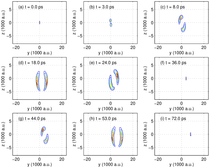
Figure 9: (color online). Contour plot snapshots of detached electron wave packet motion in the $y$-$z$ plane for the case of zero initial momentum in the $x$ direction [cf. Eq. (95)]. The static electric and magnetic field strengths are 60 V/cm and 1 T respectively. The laser pulse duration is $T_{p}=2$ ps and $t=0$ corresponds to the end of this pulse. The total electron energy is $E_{f}=8$ cm^-1.

We examine here the dynamics of a detached electron wave packet produced by a short laser pulse under the influence of crossed static electric and magnetic fields. As discussed in Refs. Peter93 ; Peter93b , the oscillatory part of the photodetachment cross section produced by a monochromatic laser field may be associated with those closed orbits that exist for a given value of the photon energy. As discussed in the previous section, the oscillatory part of the effective cross section produced by a short laser pulse is suppressed when the pulse duration is smaller than the classical orbit periods of those orbits that exist at the energy being considered. (See Du95 for the related pure static electric field case.) From the correspondence between classical and quantum mechanics, we expect to observe that the detached electron wave packets produced by short laser pulses will trace the paths of allowed classical closed orbits.

In order to illustrate the quantum wave packet motion corresponding to the classical dynamics, we shall only consider two-dimensional quantum motion by imposing the restriction $p_{x}=0$. As discussed above, the $x$ component of the momentum has to be zero in order for there to be any closed orbits. In this case, the time-dependent electron wave packet in coordinate space is given by

$$\psi_{\text{sgl}}^{\text{wvpk}}(0,y,z,t)=\frac{1}{2\pi}\int_{-\infty}^{\infty}\psi_{\text{sgl}}^{\text{wvpk}}(0,p_{y},z,t)e^{ip_{y}y},$$ (95)

which is the Fourier transform of Eq. (40), taking $p_{x}=0$. A similar Fourier transform can be employed for the double pulse case in Eq. (45).

In Figs. 9-11 we present snapshots of the detached electron wave packet for the case of a single laser pulse of the form (6) with pulse duration $T_{p}=2$ ps. The time evolution starts from $t_{0}=-T_{p}$. The static electric and magnetic field strengths are taken to be 60 V/cm and 1 T respectively in all cases. Note that the cyclotron period is $T_{B}=35.72$ ps for $B=1$ T.

Figure 10: (color online). Same as Fig. 9 but for a total detached electron energy of $E_{f}=15.9$ cm^-1.

In Fig. 9, we take the total energy $E_{f}$ to be 8 cm^-1. There is only one classical closed orbit for this energy and these static field parameters. The return time of the closed orbit is calculated to be $T_{\rm{ret}}^{0}=24.1$ ps (0.674 $T_{B}$). In Fig. 9(a), we see that two electron wave packets are created at the peak intensity of the laser pulse on either side of the $z=0$ axis, which correspond to electrons being ejected either along or opposite to the direction of increasing static electric field, $E_{S}$ (cf. Fig. 1). After the end of the pulse in (b), the two electron wave packets move apart. However, as time increases we see in (c) that both wave packets are turned back by the external magnetic field. As shown in (c) and (d), each wave packet undergoes considerable spatial spreading. The most interesting plot is shown in (e), where we see a large portion of the left hand wave packet sweep through the residual core (at the origin). We note that the time corresponding to this snapshot is exactly the return time of the only classical closed orbit in the present case. It is return of this piece of the wave packet that leads to the regular sinusoidal oscillation one sees in Fig. 5(a) below 15.9 cm^-1. As the time approaches 1 $T_{B}$ in (f), we see that the two wave packets refocus on the positive $y$ axis (the direction of drift motion) and that they pass through each other and continue their rotational motion during the next cyclotron period. However, owing to the drift motion along the $y$-axis, we see in (h) that the left hand wave packet is no longer able to return to the atomic core in the second cyclotron cycle for this total energy. The two wave packets do refocus further along the positive $y$-axis again at 2 $T_{B}$, as shown in (i).

Figure 11: (color online). Same as Figs. 10(e), (f), (g) and (h) except that the wave packet amplitudes are shown here in three-dimensions rather than as contour plots. Note the scale change in panel (b), which shows the re-focusing of the wave packet amplitude along the drift axis (i.e., away from the atomic core at the origin).

We note that the refocusing and the drift of the electron wave packets are exactly analogous to the classical dynamics discussed by Peters and Delos in Peter93 . They showed that classical orbits with different initial conditions will refocus at various points along the drift axis. We note also that pump-probe experimental studies of the related problem of the motion of pump-laser-produced Rydberg-state electron wave packets in the Rubidium atom in the presence of crossed fields have found enhancements of probe laser-produced ionization signals when the delay of the probe laser equals the orbital period of the appropriate closed classical orbit for this related problem Yeaz93 .

We present similar snapshots in time for the increased energy of 15.9 cm^-1 in Fig. 10. At this energy, the first so-called boundary orbit Peter93 may be populated (cf. Eq. (89) for $j=1$). There are thus two classical closed orbits that exist at this total energy, whose return times are 27.4 ps (0.766 $T_{B}$) and 48.8 ps (1.366 $T_{B}$). In Figs. 10(e) and 10(g) we see that different parts of the quantum electron wave packet return to the atomic core at these two times. The most distinctive feature of the part of the electron wave packet that returns to the origin at approximately 49 ps (cf. Fig. 10(g)) (which corresponds to the higher energy, classical boundary orbit) is that most of the arc in (g) passes through the atomic core at the origin (which we have confirmed by observing the motion of the electron wave packet on a finer time scale). We note also that the energy of the classical boundary orbit corresponds to the abruptly increased amplitude of the oscillatory part of the cross section seen in Fig. 5(a) around the energy location 15.9 cm^-1 indicated by the first dashed line.

The fact that electron wave packet amplitudes return to the region of the atomic core implies the possibility of modulating the detachment cross section, analogously to the case of a monochromatic laser, as shown in Figs. 4 and 5. However, the present wave packet studies show why for the crossed field case the modulation of the cross section is very small. Consider the three dimensional wave packet snapshots in Fig. 11, which are calculated for times corresponding to those in Figs. 10(e), (f), (g), and (h). Owing to the spreading of the electron wave packet, when it returns to the origin the part of the wave packet that overlaps the origin is nearly two orders of magnitude smaller than the probability in (f), in which the wave packet re-focuses along the drift axis, i.e., away from the origin. Because of such wave packet spreading and drift away from the origin, modulation of the photodetachment cross section in the crossed static field case is necessarily small. For similar reasons, the use of short pulse, pump-probe type techniques to control the photodetachment cross section in the crossed static field case also results in only small modulations of the cross section, as we discuss next.

IV.2.3 Pump-Probe Coherent Control of the Effective Photodetachment Cross Section Using Short Laser Pulses

The idea of using laser pulses shorter than electron wave packet orbital periods to control electron wave packet motion was initially formulated theoretically for Rydberg (i.e., bound) electron wave packets ARZ1986 . This idea was extended theoretically to photodetached (i.e., continuum) electron wave packets in the presence of external static fields, including static electric Wang93 and parallel static electric and magnetic Wang95 fields. Experimentally, short pulse, pump-probe studies of photodetachment of O^- in the presence of a static magnetic field demonstrated Ramsey interference between photodetached electron wave packets Yuki97 . Such Ramsey interference may also be demonstrated in the present crossed electric and magnetic field case.

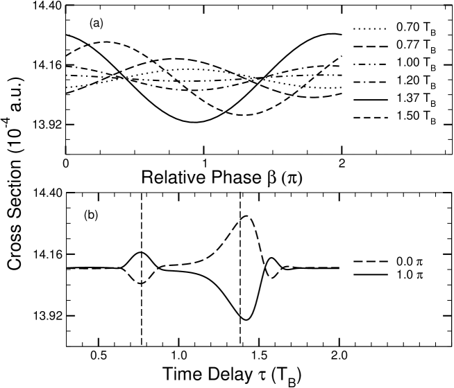
Figure 12: The effective cross section for the double laser pulse case as modulated by: (a) the relative phase between the two pulses for several time delays, as indicated; (b) the time delay between the two pulses for two fixed relative phases, 0 and $\pi$.

In Fig. 12 we present the effective total photodetachment cross section (cf. Eq. (67)) as a function of the relative phase $\beta$ and the time delay $\tau$ between two laser pulses (cf. Eq (41)) for a total detached electron energy of 15.9 cm^-1 and for $E_{S}=60$ V/cm and $B=1$ T. The pulse duration $T_{p}$ of both pulses is taken to be 4 ps. Fig. 12(a) shows the dependence of the effective cross section on the relative phase, $\beta$, for six time delays, $\tau$, between the pulses. One observes that the modulations of the cross section have local maxima for time delays of 0.77 $T_{B}$ ($\approxeq 27.5$ ps) and 1.37 $T_{B}$ ($\approxeq 49$ ps), which are precisely the return times of the two allowed classical closed orbits for a total electron energy of 15.9 cm^-1. However, the modulation of the cross section for the larger time delay is much greater than for the smaller time delay, which is consistent with the extent of electron wave packet overlap with the origin shown in Figs. 10(e) and (g). In other words, in the latter case a large portion of the wave packet passes over the origin, which makes the Ramsey interference with the newly produced wave packet amplitude (due to the second pulse) of greater amplitude.

Fig. 12(b) shows the dependence of the effective cross section on the time delay, $\tau$, for two relative phases, $\beta$, between the pulses: 0 and 1 $\pi$. Fig. 12(b) clearly shows that the maxima and minima in the effective cross section as a function of the time delay between the pulses occur for time delays of 0.77 $T_{B}$ ($\approxeq 27.5$ ps) and 1.37 $T_{B}$ ($\approxeq 49$ ps), which are the orbital periods of the two allowed classical closed orbits. We see once again that the modulation of the effective cross section is much larger for the classical closed orbit having the larger time delay, as explained above.

V Conclusions

In this paper we have presented a detailed quantum mechanical analysis of detachment of a weakly bound electron by a short laser pulse in the presence of crossed static electric and magnetic fields. For specificity, we have chosen the parameters of the initial state of the weakly bound electron as those appropriate for the outer electron in H^-. In particular we have presented an analytic expression for the final state electron wave function, i.e., the wave function for an electron moving in the field of a laser pulse of arbitrary intensity as well as in crossed static electric and magnetic fields of arbitrary strengths. The general detachment probability formulas we present may therefore be used to analyze multiphoton detachment in crossed fields (although we have not presented this analysis here, but instead have focused on the weak laser field case).

Based upon our analytic results for the detachment probability by a short laser pulse, we have defined an effective detachment cross section for the short pulse case that is shown to reduce, in the long pulse limit to results of others for the monochromatic, plane wave case. Our effective cross section formula allows us to demonstrate the effects of the laser pulse duration, such as, e.g., that for pulse durations shorter than the period of a particular classical closed orbit, the features of that closed orbit in the photodetachment spectrum (for the plane wave case) will simply vanish. By means of a stationary phase analysis, we have derived a condition for the existence of closed classical orbits that agrees exactly with that obtained by Peters and Delos by a purely classical analysis Peter93 . We have also illustrated the bifurcation of the closed classical orbits at the so-called boundary energies Peter93 by Fourier transforming the oscillatory part of our quantum cross section (in the long pulse limit) over various ranges of the final state electron energy.

Finally, our analysis of the motion of detached electron wave packets produced by a short laser pulse provides a direct comparison of quantum and classical features for the crossed static electric and magnetic field problem. We find that the dynamics of our two-dimensional detached electron wave packets are consistent with the predictions of closed classical orbit theory Peter93 . We have also shown that wave packet spreading and the fact that wave packet refocusing only occurs at the origin in the drift frame means that control of electron detachment in crossed static fields by means of laser pulses is less effective than in the parallel static electric and magnetic field case Wang95 .

Appendix A Analytical Wave Function for Free Electron Motion in a Laser Field and Crossed Static Electric and Magnetic Fields

In this appendix we give the details of the solution of Eq. (10), which describes free electron motion in a laser field in the presence of crossed static electric and magnetic fields. The configuration of the external fields is shown in Fig. 1. The solution is clearly separable in momentum space and has the following form:

$$\psi_{f}^{(p)}(\mathbf{p},t) = \psi_{x}(p_{x},t)\psi_{y}(p_{y},t)\psi_{z}(p_{z},t)\exp\left[-i\frac{1}{2c^{2}}\int_{-\infty}^{t}A_{L}^{2}(t^{\prime})dt^{\prime}\right]$$ (96)

$$= \delta(p_{x}-k_{x})\delta(p_{y}-k_{y})\psi_{z}(p_{z},t)$$

$$\times\exp\left[-i\frac{1}{2}(k_{x}^{2}+k_{y}^{2})t-i\frac{1}{2c^{2}}\int_{-\infty}^{t}A_{L}^{2}(t^{\prime})dt^{\prime}\right],$$

where the $z$ component of the final state wave function satisfies the following equation:

$$i\frac{\partial}{\partial t}\psi_{z}(p_{z},t)=\left[-\frac{1}{2}\omega_{c}^{2}\frac{\partial^{2}}{\partial p_{z}^{2}}-i\omega_{c}\left(p_{y}-\frac{E_{S}}{\omega_{c}}\right)\frac{\partial}{\partial p_{z}}+\frac{1}{2}p_{z}^{2}+\frac{1}{c}p_{z}A_{L}(t)\right]\psi_{z}(p_{z},t).$$ (97)

In order to solve Eq. (97), we make the following substitution:

$$\psi_{z}(p_{z},t)=\exp\left[-i\frac{1}{\omega_{c}}(k_{y}-\frac{E_{S}}{\omega_{c}})p_{z}\right]\psi_{z1}(p_{z},t),$$ (98)

which serves to eliminate the term involving the first derivative of $p_{z}$ from the equation satisfied by $\psi_{z1}(p_{z},t)$,

$$i\frac{\partial}{\partial t}\psi_{z1}(p_{z},t)=\left[-\frac{1}{2}\omega_{c}^{2}\frac{\partial^{2}}{\partial p_{z}^{2}}+\frac{1}{2}p_{z}^{2}+\frac{1}{c}p_{z}A_{L}(t)-\frac{1}{2}\left(k_{y}-\frac{E_{S}}{\omega_{c}}\right)^{2}\right]\psi_{z1}(p_{z},t).$$ (99)

Upon making the substitution,

$$\psi_{z1}(p_{z},t)=\exp\left[i\frac{1}{2}\left(k_{y}-\frac{E_{S}}{\omega_{c}}\right)^{2}t\right]\psi_{z2}(p_{z},t),$$ (100)

Eq. (99) gives the following equation for $\psi_{z2}(p_{z},t)$:

$$i\frac{\partial}{\partial t}\psi_{z2}(p_{z},t)=\left[-\frac{1}{2}\omega_{c}^{2}\frac{\partial^{2}}{\partial p_{z}^{2}}+\frac{1}{2}p_{z}^{2}+\frac{1}{c}A_{L}(t)p_{z}\right]\psi_{z2}(p_{z},t).$$ (101)

Eq. (101) has the form of the equation for a forced harmonic oscillator, which can be solved exactly Husi53 :

$$\psi_{z2}(p_{z},t)=\exp\left[-i\varepsilon_{n_{z}}t+i\frac{\dot{\xi}(t)}{\sqrt{\omega_{c}^{3}}}\sqrt{2}\zeta_{p_{z}}+i\int_{-\infty}^{t}L(t^{\prime})dt^{\prime}\right]\omega_{c}^{-1/4}g_{n_{z}}\left(\sqrt{2}\zeta_{p_{z}}\right),$$ (102)

where $\zeta_{p_{z}}$ and $\varepsilon_{n_{z}}$ are given by Eqs. (18) and (20) respectively. The function $\xi(t)$ is related to the vector potential of the laser pulse and satisfies the differential equation given in Eq. (22). The function $L(t)$ is defined in Eq. (21) in terms of $\xi(t)$. In Eq. (102), the function $g_{n_{z}}\left(x\right)$ is defined by Eq. (14). Note that $g_{n_{z}}(x)$ is normalized, i.e.,

$$\int_{-\infty}^{\infty}[g_{n_{z}}]^{2}\,dx=1.$$ (103)

We note also that $g_{n_{z}}(x)$ is simply proportional to a parabolic cylinder function (see Eq. 19.13.1 of Ref. Abra65 ):

$$g_{n_{z}}(x)=\frac{1}{\sqrt{n_{z}!\sqrt{\pi}}}U\left(-n_{z}-\frac{1}{2}\sqrt{2}x\right).$$ (104)

Combining Eqs. (98),  (100), and (102), we find for the solution of Eq. (97),

$$\psi_{z}(p_{z},t) = \exp\left[-ib(k_{y},t)\sqrt{2}\zeta_{p_{z}}\right]\omega_{c}^{-1/4}g_{n_{z}}\left(\sqrt{2}\zeta_{p_{z}}\right)$$ (105)

$$\times\exp\left[-i\varepsilon_{n_{z}}t-i\frac{1}{\sqrt{\omega_{c}}}\zeta_{k_{y}}\xi(t)+i\frac{1}{2}\omega_{c}\zeta_{k_{y}}^{2}t+i\int_{-\infty}^{t}L(t^{\prime})dt^{\prime}\right],$$

where $b(k_{y},t)$ and $\zeta_{k_{y}}$ are given by Eq. (17) and (19) respectively. Finally, substituting Eq. (105) into Eq. (96) gives us the analytical expression for the final state wave function in momentum space given in Eq. (13).

Appendix B Solution of Eq. (22) for $\xi(t)$

In this appendix we present the solution for the laser-field-dependent function $\xi(t)$, which satisfies the differential equation (22). The corresponding Green’s function satisfies,

$$\ddot{G}(t,t^{\prime})+\omega_{c}^{2}G(t,t^{\prime})=\delta(t-t^{\prime}),$$ (106)

whose solution is:

$$G(t,t^{\prime})=\frac{1}{2\pi}\int_{-\infty}^{\infty}\frac{e^{i\omega^{\prime}(t-t^{\prime})}}{\omega_{c}^{2}-\omega^{\prime 2}}d\omega^{\prime}.$$ (107)

In terms of this Green’s function, the solution of Eq. (22) is:

$$\xi(t) = \int_{-\infty}^{\infty}G(t,t^{\prime})\left[-\frac{\omega_{c}^{2}}{c}A_{L}(t^{\prime})\right]dt^{\prime}$$ (108)

$$= \frac{\omega_{c}^{2}}{2\pi}\int_{-\infty}^{\infty}d\omega^{\prime}\frac{e^{i\omega^{\prime}t}}{\omega_{c}^{2}-\omega^{\prime 2}}\int_{-\infty}^{\infty}dt^{\prime}\left[-\frac{1}{c}A_{L}(t^{\prime})\right]e^{-i\omega^{\prime}t^{\prime}}.$$

Using the definitions in Eqs. (6) and (9), the integral over $t^{\prime}$ can be evaluated (using integration by parts) to obtain,

$$I(\omega^{\prime}) = \int_{-\infty}^{\infty}dt^{\prime}\left[-\frac{1}{c}A_{L}(t^{\prime})\right]e^{-i\omega^{\prime}t^{\prime}}$$ (109)

$$= \frac{\sqrt{\pi}}{i\omega^{\prime}}\frac{E_{0}}{2i\alpha}W(\omega^{\prime}),$$

in which the function $W(\omega^{\prime})$ is defined by

$$W(\omega^{\prime})=e^{-\frac{(\omega-\omega^{\prime})^{2}}{4\alpha^{2}}+i(\omega-\omega^{\prime})\tau+i\beta}-e^{-\frac{(\omega+\omega^{\prime})^{2}}{4\alpha^{2}}-i(\omega+\omega^{\prime})\tau-i\beta},$$

and where it has been assumed that $A_{L}(-\infty)=A_{L}(\infty)=0$.

Thus $\xi(t)$ is now given by

$$\xi(t) = \frac{\omega_{c}^{2}}{2\pi}\int_{-\infty}^{\infty}d\omega^{\prime}\frac{e^{i\omega^{\prime}t}}{\omega_{c}^{2}-\omega^{\prime 2}}\frac{\sqrt{\pi}}{i\omega^{\prime}}\frac{E_{0}}{2i\alpha}W(\omega^{\prime})$$ (110)

$$= \frac{E_{0}}{2\alpha i}\frac{\sqrt{\pi}}{2}\left[I_{0}(t)+I_{1}(t)+I_{2}(t)\right],$$

where we have defined the following three integrals over $\omega^{\prime}$:

$$I_{0}(t) = \frac{1}{\pi i}\int_{-\infty}^{\infty}d\omega^{\prime}\frac{1}{\omega^{\prime}}W(\omega^{\prime})e^{i\omega^{\prime}t},$$ (111)

$$I_{1}(t) = -\frac{1}{2\pi i}\int_{-\infty}^{\infty}d\omega^{\prime}\frac{1}{\omega^{\prime}-\omega_{c}}W(\omega^{\prime})e^{i\omega^{\prime}t},$$ (112)

$$I_{2}(t) = -\frac{1}{2\pi i}\int_{-\infty}^{\infty}d\omega^{\prime}\frac{1}{\omega^{\prime}+\omega_{c}}W(\omega^{\prime})e^{i\omega^{\prime}t}.$$ (113)

B.1 Calculation of $I_{0}(t)$, $I_{1}(t)$ and $I_{2}(t)$

Consider first $I_{1}(t)$, which satisfies the following relation:

$$\frac{d}{dt}[e^{-i\omega_{c}t}I_{1}(t)] = -\frac{1}{2\pi}\int_{-\infty}^{\infty}d\omega^{\prime}W(\omega^{\prime})e^{i\left(\omega^{\prime}-\omega_{c}\right)t}$$

$$= -\frac{i2\alpha}{\sqrt{\pi}}e^{-\alpha^{2}(t-\tau)^{2}-i\omega_{c}t}\sin(\omega t+\beta).$$

Thus, we have that

$$I_{1}(t) = -\frac{i2\alpha}{\sqrt{\pi}}e^{i\omega_{c}t}\int_{-\infty}^{t}e^{-\alpha^{2}(t^{\prime}-\tau)^{2}-i\omega_{c}t^{\prime}}\sin(\omega t^{\prime}+\beta)dt^{\prime}$$ (115)

$$= -\frac{1}{2}e^{i\omega_{c}(t-\tau)}\left[\mathop{\rm erf}\left(\alpha(t-\tau)-\frac{i(\omega-\omega_{c})}{2\alpha}\right)+1\right]e^{-\frac{(\omega-\omega_{c})^{2}}{4\alpha^{2}}+i\beta+i\omega\tau}$$

$$+\frac{1}{2}e^{i\omega_{c}(t-\tau)}\left[\mathop{\rm erf}\left(\alpha(t-\tau)+\frac{i(\omega+\omega_{c})}{2\alpha}\right)+1\right]e^{-\frac{(\omega+\omega_{c})^{2}}{4\alpha^{2}}-i\beta-i\omega\tau}.$$

Replacing $\omega_{c}$ by $-\omega_{c}$ in the above formula, we get

$$I_{2}(t) = -\frac{1}{2}e^{-i\omega_{c}(t-\tau)}\left[\mathop{\rm erf}\left(\alpha(t-\tau)-\frac{i(\omega+\omega_{c})}{2\alpha}\right)+1\right]e^{-\frac{(\omega+\omega_{c})^{2}}{4\alpha^{2}}+i\beta+i\omega\tau}$$ (116)

$$+\frac{1}{2}e^{-i\omega_{c}(t-\tau)}\left[\mathop{\rm erf}\left(\alpha(t-\tau)+\frac{i(\omega-\omega_{c})}{2\alpha}\right)+1\right]e^{-\frac{(\omega-\omega_{c})^{2}}{4\alpha^{2}}-i\beta-i\omega\tau}.$$

Setting $\omega_{c}$ equal to zero in Eq. (115) and multiplying by a factor of $-2$, we get

$$I_{0}(t) = -\left[\mathop{\rm erf}\left(\alpha(t-\tau)+\frac{i\omega}{2\alpha}\right)+1\right]e^{-\frac{\omega^{2}}{4\alpha^{2}}-i\beta-i\omega\tau}$$ (117)

$$+\left[\mathop{\rm erf}\left(\alpha(t-\tau)-\frac{i\omega}{2\alpha}\right)+1\right]e^{-\frac{\omega^{2}}{4\alpha^{2}}+i\beta+i\omega\tau}.$$

B.2 Some Relations for $\xi(t)$ and Its Derivatives

From Eqs. (110) and (115) (and equations similar to (115) for $I_{0}(t)$ and $I_{2}(t)$), we have that

$$\dot{\xi}(t) = \frac{E_{0}\sqrt{\pi}}{4\alpha i}\left[\dot{I}_{0}(t)+\dot{I}_{1}(t)+\dot{I}_{2}(t)\right]$$ (118)

$$= \frac{E_{0}\,\omega_{c}\sqrt{\pi}}{4\alpha}\left[I_{1}(t)-I_{2}(t)\right].$$ (119)

The second derivative of $\xi(t)$ is given by

$$\ddot{\xi}(t) = \frac{E_{0}\,\omega_{c}\sqrt{\pi}}{4\alpha}\left[\dot{I}_{1}(t)-\dot{I}_{2}(t)\right]$$ (120)

$$= i\frac{E_{0}\,(\omega_{c})^{2}\sqrt{\pi}}{4\alpha}\left[I_{1}(t)+I_{2}(t)\right].$$

Writing now

$$\xi(t)=\sum_{i=0}^{2}\xi_{i}(t),$$ (121)

where

$$\xi_{i}(t)=\frac{E_{0}\sqrt{\pi}}{4\alpha i}I_{i}(t),$$ (122)

Eqs. (119) and (120) give

$$\dot{\xi}(t)=i\omega_{c}\left[\xi_{1}(t)-\xi_{2}(t)\right],$$ (123)

$$\ddot{\xi}(t)=-\omega_{c}^{2}\left[\xi_{1}(t)+\xi_{2}(t)\right].$$ (124)

Substituting these equations into Eq. (22) gives:

$$\xi_{0}(t)=-\frac{1}{c}A_{L}(t).$$ (125)

B.3 Long Pulse Approximation for $\xi(t)$

In the long pulse case (in which $\alpha/\omega\ll 1$), simplified expressions can be obtained for the integrals $I_{i}(t)$ in a way similar that used in Ref. Wang95 . For example, starting from Eq. (115) one can expand the sine function in terms of exponentials and then do the resulting integration by parts, dropping terms that are of order $\alpha/\omega$ or higher, as follows:

$$I_{1}(t) = -\frac{\alpha}{\sqrt{\pi}}e^{i\omega_{c}t}\int_{-\infty}^{t}e^{-\alpha^{2}(t^{\prime}-\tau)^{2}}[e^{i(\omega-\omega_{c})t^{\prime}+i\beta}-e^{-i(\omega+\omega_{c})t^{\prime}-i\beta}]$$ (126)

$$\simeq \frac{i\alpha}{\sqrt{\pi}}e^{-\alpha^{2}(t-\tau)^{2}}\left[\frac{1}{\omega-\omega_{c}}e^{i\left(\omega t+\beta\right)}+\frac{1}{\omega+\omega_{c}}e^{-i\left(\omega t+\beta\right)}\right].$$ (127)

In a similar way one may obtain the following approximate expressions for $I_{2}(t)$ and $I_{0}(t)$:

$$I_{2}(t) \simeq \frac{i\alpha}{\sqrt{\pi}}e^{-\alpha^{2}(t-\tau)^{2}}\left[\frac{1}{\omega+\omega_{c}}e^{i\left(\omega t+\beta\right)}+\frac{1}{\omega-\omega_{c}}e^{-i\left(\omega t+\beta\right)}\right],$$ (128)

$$I_{0}(t) \simeq \frac{-4i\alpha}{\sqrt{\pi}}\frac{1}{\omega}e^{-\alpha^{2}(t-\tau)^{2}}\cos\left(\omega t+\beta\right).$$ (129)

Substituting these long pulse approximations for the integrals $I_{i}(t)$ into Eq. (110), the function $\xi(t)$ in the long pulse limit is then given by Eq. (23).

References

• (1) P.A. Braun, Rev. Mod. Phys. 65, 115 (1993).
• (2) H. Crosswhite, U. Fano, K.T. Lu, and A.R.P. Rau, Phys. Rev. Lett. 42, 963 (1979).
• (3) J.C. Gay, L.R. Pendrill, and B. Cagnac, Phys. Lett. 72A, 315 (1979).
• (4) E. Korevaar and M.G. Littman, J. Phys. B 16, L437 (1983).
• (5) C.W. Clark, K.T. Lu, and A.F. Starace, Progress in Atomic Spectroscopy, Part C, ed H.J. Beyer and H. Kleinpoppen (Plenum, New York,1984), pp. 247-320.
• (6) C.W. Clark, E. Korevaar, and M.G. Littman, Phys. Rev. Lett. 54, 320 (1985).
• (7) C. Nessmann and W.P. Reinhardt, Phys. Rev. A 35, 3269 (1987).
• (8) M. Fauth, H. Walther, and E. Werner, Z. Phys. D 7, 293 (1987).
• (9) J. Hare, M. Gross, and P. Goy, Phys. Rev. Lett. 61, 1938 (1988).
• (10) G. Wiebusch, J. Main, K. Krüger, H. Rottke, A. Holle, and K.H. Welge, Phys. Rev. Lett. 62, 2821 (1989).
• (11) J.-C. Gay, D. Delande, and A. Bommier, Phys. Rev. A 39, 6587 (1989).
• (12) M.Vincke, M. LeDourneuf, and D. Baye, J. Phys. B 25, 2787 (1992).
• (13) J.A. Yeazell, G. Raithel, L. Marmet, H. Held, and H. Walther, Phys. Rev. Lett. 70, 2884 (1993).
• (14) O. Dippel, P. Schmelcher, and L.S. Cederbaum, Phys. Rev. A 49, 4415 (1994).
• (15) J. von Milczewski, G.H.F. Diercksen, and T. Uzer, Int. J. Bifurcation and Chaos 4, 905 (1994).
• (16) J. von Milczewski, G.H.F. Diercksen, and T. Uzer, Phys. Rev. Lett. 76, 2890 (1996).
• (17) J.P. Connerade, G. Droungas, N.E. Karapanagioti, and M.S. Zhang, J. Phys. B 30, 2047 (1997).
• (18) C. Neumann, R. Ubert, S. Freund, E. Flöthmann, B. Sheehy, K.H. Welge, M.R. Haggerty, and J.B. Delos, Phys. Rev. Lett. 78, 4705 (1997).
• (19) J. von Milczewski and T. Uzer, Phys. Rev. E 55, 6540 (1997).
• (20) J. von Milczewski, D. Farrelly, and T. Uzer, Phys. Rev. A 56, 657 (1997).
• (21) J.G. Rao and K.T. Taylor, J. Phys. B 30, 3627 (1997).
• (22) D.A. Sadovskii and B.I. Zhilinskii, Phys. Rev. A 57, 2867 (1998).
• (23) K. Weibert, J. Main, and G. Wunner, Ann. Phys.(N.Y.) 268, 172 (1998).
• (24) V. Averbukh, N. Moiseyev, P. Schmelcher, and L.S. Cederbaum, Phys. Rev. A 59, 3695 (1999).
• (25) R.H. Cushman and D.A. Sadovskii, Europhys. Lett. 47, 1 (1999).
• (26) R.H. Cushman and D.A. Sadovskii, Physica D 142, 166 (2000).
• (27) D.M. Wang and J.B. Delos, Phys. Rev. A 63, 043409 (2001).
• (28) T. Uzer, Phys. Scripta T90, 176 (2001).
• (29) P. Schmelcher, Phys. Rev. A 64, 063412 (2001).
• (30) J.G. Rao, D. Delande, and K.T. Taylor, J. Phys. B 35, L1 (2002).
• (31) S. Freund, R. Ubert, E. Flöthmann, K. Welge, D.M. Wang, and J.B. Delos, Phys. Rev. A 65, 053408 (2002).
• (32) J.G. Rao and K.T. Taylor, J. Phys. B 35, 2627 (2002).
• (33) G. Valent, Am. J. Phys. 71, 171 (2003).
• (34) T. Bartsch, J. Main, and G. Wunner, Phys. Rev. A 67, 063411 (2003).
• (35) A.M. Abdulla, S. Hogan, M.S. Zhan, and J.P. Connerade, J. Phys. B 37, L147 (2004).
• (36) J.P. Connerade, S.D. Hogan and A.M. Abdulla, J. Phys. B 38, S141 (2005).
• (37) G.F. Drukarev and B.S. Monozon, Zh. Eksp. Teor. Fiz. 61, 956 (1971) [Sov. Phys. JETP 34, 509 (1972)].
• (38) V.S. Popov, B.M. Karnakov, and V.D. Mur, Zh. Eksp. Teor. Fiz. 113, 1579 (1998) [JETP 86, 860 (1998)].
• (39) W.A.M. Blumberg, W.M. Itano, and D.J. Larson, Phys. Rev. A 19, 139 (1979).
• (40) J.N. Yukich, C.T. Butler, and D.J. Larson, Phys. Rev. A 55, R3303 (1997).
• (41) I.I. Fabrikant, Phys. Rev. A 43, 258 (1991).
• (42) A.D. Peters and J.B. Delos, Phys. Rev. A 47, 3020 (1993).
• (43) A.D. Peters and J.B. Delos, Phys. Rev. A 47, 3036 (1993).
• (44) Z.Y. Liu, D.H. Wang, S.L. Lin, and W.Z. Shi, Phys. Rev. A 54, 4078 (1996).
• (45) Z.Y. Liu and D.H. Wang, Phys. Rev. A 55, 4605 (1997).
• (46) Z.Y. Liu and D.H. Wang, Phys. Rev. A 56, 2670 (1997).
• (47) G. Alber and P. Zoller, Phys. Rep. 199, 2231 (1991).
• (48) H.R. Reiss, Phys. Rev. A, 22, 1786 (1980).
• (49) A.I. Nikishov and V.I. Ritus, Zh. Eksp. Teor. Fiz. 50, 255 (1966) [Sov. Phys. JETP 23, 168 (1967)].
• (50) B. Gao and A.F. Starace, Phys. Rev. A 42, 5580 (1990).
• (51) T. Ohmura and H. Ohmura, Phys. Rev. 118, 154 (1960).
• (52) H.A. Bethe and C. Longmire, Phys. Rev. 77, 647 (1950).
• (53) M.L. Du and J.B. Delos, Phys. Rev. A 38, 5609 (1988).
• (54) I.S. Gradshteyn and I.W. Ryzhik, Table of Integrals, Series, and Products, 4th ed. (Academic, New York, 1965).
• (55) Q. Wang and A.F. Starace, Phys. Rev. A 51, 1260 (1995).
• (56) Handbook of Mathematical Functions, ed. by M. Abramowitz and I.A. Stegun (Dover, New York, 1965).
• (57) B. Gao, Phys. Rev. A 41, 5039 (1990).
• (58) G. Szegö, Orthogonal polynomials (Am. Math. Soc., Providence, Rhode Island, 1939), p. 201.
• (59) Q. Wang and A.F. Starace, Phys. Rev. A 55, 815 (1997).
• (60) A.D. Peters, C. Jaffé, and J.B. Delos, Phys. Rev. Lett. 73, 2825 (1994).
• (61) Q. Wang and A.F. Starace, Phys. Rev. A 48, R1741 (1993).
• (62) M.L. Du, Phys. Rev. A 52, 1143 (1995).
• (63) Y.L. Zhao, M.L. Du, and J.M. Mao, J. Phys. B: At. Mol. Opt. Phys. 32, 1409 (1999).
• (64) B.M. Garraway and K.-A. Suominen, Rep. Prog. Phys. 58, 365 (1995).
• (65) R. Bluhm, V.A. Kostelecký, and J.A. Porter, Am. J. Phys. 64, 944 (1996).
• (66) G. Alber, H. Ritsch, and P. Zoller, Phys. Rev. A 34, 1058 (1986).
• (67) K. Husimi, Prog. Theo. Phys. 9, 381 (1953).