“Breathing” rogue wave observed in numerical experiment

Abstract

Numerical simulations of the recently derived fully nonlinear equations of motion for weakly three-dimensional water waves [V.P. Ruban, Phys. Rev. E 71, 055303(R) (2005)] with quasi-random initial conditions are reported, which show the spontaneous formation of a single extreme wave on the deep water. This rogue wave behaves in an oscillating manner and exists for a relatively long time (many wave periods) without significant change of its maximal amplitude.

I Introduction

The rogue waves (rare extreme events on a relatively calm sea surface, alternatively called freak, killer, or giant waves), for a long time a part of marine folklore, since 1970’s have been methodically documented by oceanographers (see review Kharif-Pelinovsky for examples and some relevant statistics). From the viewpoint of nonlinear science, a rogue wave is an extremely nonlinear object — typically, the amplitude of a freak wave in maximum is close to the amplitude of the corresponding limiting Stokes wave, that is $h/\lambda\approx 0.10\dots 0.14$, where $h$ is the peak-to-trough height, and $\lambda$ is the length of the wave DZ2005Pisma . Therefore, for adequate quantitative investigation, this phenomenon requires fully nonlinear equations and accurate numerical methods. For two-dimensional (2D) potential flows with a free boundary, a very efficient numerical scheme has been developed recently by Zakharov and co-workers ZDV2002 . The scheme is based on exact (1+1)-dimensional equations of motion written for the surface shape and for the boundary value of the velocity potential in terms of the so called conformal variables (the corresponding exact 2D theory is described in Refs. DKSZ96 ; DZK96 ; DLZ95 ; D2001 ; CC99 ; R2004PRE ; R2005PLA ). The method extensively uses algorithms of the discrete fast Fourier transform (FFT). With applying this method, impressive computations have been performed, where a numerical giant wave developed due to the Benjamin-Feir (modulational) instability Benjamin-Feir ; Zakharov67 from a slightly perturbed Stokes wave. The spatial resolution in these numerical experiments was up to $2\cdot 10^{6}$ points DZ2005Pisma . As to three-dimensional (3D) flows, unfortunately, a similar exact and compact (2+1)-dimensional form of equations is absent. Therefore “exact” 3D simulations are currently based on the rather expensive boundary element method (BEM) and its modifications (see Clamond-Grue-2001 ; Fructus_et_al_2005 ; Grilli ; GuyenneGrilli2006 , and references therein). Since the underlying algorithms of BEM are quite complicated, the best practically achieved spatial resolutions on the free surface for essentially 3D waves are typically few tens multiplied by few tens, as in the recent works Fructus_et_al_2005 ; Grilli ; GuyenneGrilli2006 . Definitely, this is not sufficient to simulate large wave systems with dozens and hundreds waves, as it is necessary for practical applications. We exclude here the approximate equations describing wave envelopes Dysthe1979 ; TKDV2000 ; OOS2000 ; Janssen2003 , because they are not appropriate in real situations when many random waves with very different wave vectors and amplitudes are excited. Other approximate equations, for instance the weakly nonlinear Zakharov equations Z1999 ; OOSRPZB2002 ; DKZ2004 ; LZ2005 , are only good if the wave steepness is small, but this is clearly not the case for the extreme waves. However, though rogue waves are strongly nonlinear, and the wave steepness cannot serve anymore as a small parameter of the theory, nevertheless another small parameter may exist in the system. Namely, practically important is the situation when relatively long (much longer than a typical wave length) wave crests are oriented along a definite horizontal direction. For such weakly 3D flows, the advantages of the conformal variables are almost recovered, as it has been explained in Refs. R2005PRE ; RD2005PRE . In the cited papers, the noncanonical Hamiltonian description in terms of the conformal variables has been generalized from 2D to 3D potential inviscid flows with a free surface, and the asymptotic expansion of the Hamiltonian functional on the small parameter $\epsilon=(l_{x}/l_{q})^{2}$ has been suggested, where $l_{x}$ is a typical wave length, and $l_{q}$ is a large transversal scale along the wave crests. In particular, the first-order 3D corrections have been calculated explicitly. What is important, all linear operators coming into the equations are diagonal in the Fourier representation. Therefore a relatively high spatial resolution ($16384\times 256$ in Ref.RD2005PRE ) for the corresponding numerical algorithm has been possible due to the large number of local operations that result from the Fourier diagonalization. In Ref. RD2005PRE some numerical results have been presented, for non-random initial conditions and typical dimensionless wave numbers about 20.

In the present work another numerical experiment is reported, which is more close to reality. Main wave numbers now are about 50, and the computations start with a quasi-random initial state (shown in Fig. 1). Concerning efficiency of the numerical implementation, it should be noted that with the FFTW library FFTW3 , it takes less than 2 min to perform one step of the Runge-Kutta-4 numerical integration on an Intel Pentium 4 CPU 3.60GHz with 2048M memory, for the maximal possible spatial resolution $16384\times 512$. Here a giant wave formation has been observed as well, but contrary to the previous computations DZ2005Pisma and RD2005PRE , this freak wave is not breaking, but it exists for many wave periods without tendency towards increasing or decreasing its maximal amplitude (which in this case is distinctly less than the limiting Stokes wave amplitude, see Figs. 2-3). During the life time, the rogue wave behaves in an oscillating manner, with the highest crest being alternately ahead or behind of the deepest trough. Observation of such kind of behavior is important for better understanding of the rogue wave phenomenon.

Figure 1: (Color online). Map of the free surface at $t=0$.

Figure 2: Maximum wave height versus dimensionless time.

Figure 3: Wave profiles at $t=50$.

II Equations of motion

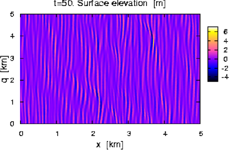
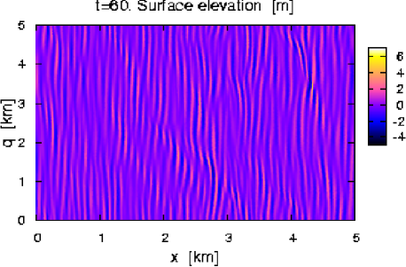
Figure 4: (Color online). Top: map of the free surface at $t=50$ (7 min 30 sec). The rogue wave has coordinates $x\approx 3.7$ km, $q\approx 3.7$ km. Middle: map at $t=60$ (9 min 1 sec). The rogue wave is at $x\approx 4.3$ km, $q\approx 3.4$ km. Bottom: map at $t=91$ (13 min 40 sec). The rogue wave is at $x\approx 1.3$ km, $q\approx 2.8$ km, and a specific wave pattern behind of it is visible.

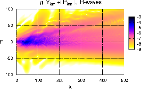
Figure 5: (Color online). Spectrum of the right-propagating waves at $t=50$. Here shown is $\log_{10}|Y_{km}+iP_{km}|$, where $P_{km}=(k^{2}+m^{2})^{1/4}\psi_{km}$.

Figure 6: Distribution of the surface elevation $y(x,q)$ at $t=50$ (no averaging over the time is done).

Here it is necessary to present the equations that were simulated. Their detailed derivation and discussion can be found in Refs. R2005PRE ; RD2005PRE . We use Cartesian coordinates $x,q,y$, with $y$ axis up-directed. The symbol $z$ denotes the complex combination: $z\equiv x+iy$. For every value of $q$, at any time moment $t$, there exists an analytical function $z(u+iv,q,t)$ which determines a conformal mapping of the lower half-plane of a complex variable $w=u+iv$ on a region below the free surface. A shape of the free surface is given in a parametric form:

$$Z=X+iY=z(u,q,t)=u+(i-\hat{H})Y(u,q,t).$$ (1)

The Hilbert operator $\hat{H}$ is diagonal in the Fourier representation: it multiplies the Fourier-harmonics

$$Y_{km}(t)\equiv\int Y(u,q,t)e^{-iku-imq}du\,dq$$

by $[i\,\mbox{sign\,}k]$, so that

$$\hat{H}Y(u,q,t)=\int[i\,\mbox{sign\,}k]Y_{km}(t)e^{iku+imq}{dk\,dm}/({2\pi})^{2}.$$ (2)

Thus, the first unknown function is $Y(u,q,t)$. The second unknown function is the boundary value $\psi(u,q,t)$ of the velocity potential,

$$\psi(u,q,t)=\int\psi_{km}(t)e^{iku+imq}{dk\,dm}/({2\pi})^{2}.$$

Correspondingly, we have two main equations of motion. They are written below in a Hamiltonian non-canonical form involving the variational derivatives $(\delta{\cal K}/\delta\psi)$ and $({\delta{\cal K}}/{\delta Z})$, where ${\cal K}\{\psi,Z,\bar{Z}\}$ is the kinetic energy. The first equation is the so called kinematic condition on the free surface:

$$Z_{t}=iZ_{u}(1+i\hat{H})\left[\frac{(\delta{\cal K}/\delta\psi)}{|Z_{u}|^{2}}\right].$$ (3)

The second equation is the dynamic condition (Bernoulli equation):

$$\psi_{t} = -g\,\mbox{Im\,}Z-\psi_{u}\hat{H}\left[\frac{(\delta{\cal K}/\delta\psi)}{|Z_{u}|^{2}}\right]$$ (4)

$$+ \frac{\mbox{Im}\left((1-i\hat{H})\left[2({\delta{\cal K}}/{\delta Z})Z_{u}+({\delta{\cal K}}/{\delta\psi})\psi_{u}\right]\right)}{|Z_{u}|^{2}},$$

where $g$ is the gravitational acceleration. Equations (3) and (4) completely determine evolution of the system, provided the kinetic energy functional ${\cal K}\{\psi,Z,\bar{Z}\}$ is explicitly given. Unfortunately, in 3D there is no exact compact expression for ${\cal K}\{\psi,Z,\bar{Z}\}$. However, for long-crested waves propagating mainly in the $x$ direction (the parameter $\epsilon\sim(l_{x}/l_{q})^{2}\ll 1$), we have an approximate kinetic-energy functional in the form

$${\cal K}\approx\tilde{\cal K}=-\frac{1}{2}\int\psi\hat{H}\psi_{u}\,du\,dq+\tilde{\cal F},$$ (5)

where the first term describes purely 2D flows, and weak 3D corrections are introduced by the functional $\tilde{\cal F}$:

$$\tilde{\cal F} = \frac{i}{8}\int(Z_{u}\Psi_{q}-Z_{q}\Psi_{u})\hat{G}\overline{(Z_{u}\Psi_{q}-Z_{q}\Psi_{u})}\,du\,dq$$ (6)

$$+ \frac{i}{16}\int\Bigg{\{}\left[(Z_{u}\Psi_{q}-Z_{q}\Psi_{u})^{2}/{Z_{u}}\right]\,\hat{E}\overline{(Z-u)}$$

$$\qquad-(Z-u)\,\hat{E}\overline{\left[(Z_{u}\Psi_{q}-Z_{q}\Psi_{u})^{2}/{Z_{u}}\right]}\Bigg{\}}\,du\,dq.$$

Here $\Psi\equiv(1+i\hat{H})\psi$, and the operators $\hat{G}$ and $\hat{E}$ are diagonal in the Fourier representation:

$$G(k,m)=\frac{-2i}{\sqrt{k^{2}+m^{2}}+|k|},$$ (7)

$$E(k,m)=\frac{2|k|}{\sqrt{k^{2}+m^{2}}+|k|}.$$ (8)

A difference between the above expression (5) and the unknown true water-wave kinetic energy functional is of order $\epsilon^{2}$, since $G(k,0)=1/(ik)$ for positive $k$, and $E(k,0)=1$ (see Refs. R2005PRE ; RD2005PRE ). Besides that, the linear dispersion relation resulting from $\tilde{\cal K}$ is correct in the entire Fourier plane (it should be noted that in Ref. RD2005PRE another approximate expression for $\tilde{\cal K}$ was used, also resulting in the first-order accuracy on $\epsilon$ and correct linear dispersion relation). Thus, we have $({\delta{\cal K}}/{\delta\psi})\approx({\delta\tilde{\cal K}}/{\delta\psi})$ and $({\delta{\cal K}}/{\delta Z})\approx({\delta\tilde{\cal F}}/{\delta Z})$ in equations (3-4), with explicit expressions closing the system:

$$\frac{\delta\tilde{\cal K}}{\delta\psi}=-\hat{H}\psi_{u}+2\,\mbox{Re\,}\left[(1-i\hat{H})\frac{\delta\tilde{\cal F}}{\delta\Psi}\right],$$ (9)

$$\frac{\delta\tilde{\cal F}}{\delta\Psi} = \frac{i}{8}Z_{q}\hat{\partial}_{u}\Big{[}\hat{G}\overline{(Z_{u}\Psi_{q}-Z_{q}\Psi_{u})}$$ (10)

$$\qquad\qquad+(\Psi_{q}-Z_{q}\Psi_{u}/{Z_{u}})\hat{E}\overline{(Z-u)}\Big{]}$$

$$-\frac{i}{8}\,Z_{u}\,\hat{\partial}_{q}\Big{[}\hat{G}\overline{(Z_{u}\Psi_{q}-Z_{q}\Psi_{u})}$$

$$\qquad\qquad+(\Psi_{q}-Z_{q}\Psi_{u}/{Z_{u}})\hat{E}\overline{(Z-u)}\Big{]},$$

$$\frac{\delta\tilde{\cal F}}{\delta Z} = -\frac{i}{8}\Psi_{q}\hat{\partial}_{u}\Big{[}\hat{G}\overline{(Z_{u}\Psi_{q}-Z_{q}\Psi_{u})}$$ (11)

$$\qquad\qquad+(\Psi_{q}-Z_{q}\Psi_{u}/{Z_{u}})\hat{E}\overline{(Z-u)}\Big{]}$$

$$+\frac{i}{8}\,\Psi_{u}\,\hat{\partial}_{q}\Big{[}\hat{G}\overline{(Z_{u}\Psi_{q}-Z_{q}\Psi_{u})}$$

$$\qquad\qquad+(\Psi_{q}-Z_{q}\Psi_{u}/{Z_{u}})\hat{E}\overline{(Z-u)}\Big{]}$$

$$+\frac{i}{16}\,\Big{[}\hat{\partial}_{u}[(\Psi_{q}-Z_{q}\Psi_{u}/Z_{u})^{2}\hat{E}\overline{(Z-u)}]$$

$$\qquad\qquad\qquad-\hat{E}\overline{(\Psi_{q}-Z_{q}\Psi_{u}/{Z_{u}})^{2}{Z_{u}}}\Big{]}.$$

III Results of the numerical experiment

(a)

(b)

(c)

(d)

Figure 7: Rogue wave profiles at $t=45$, $t=50$, $t=55$, and $t=60$.

Following the procedure described in Ref. RD2005PRE , a numerical experiment has been performed, which is described below. A square $5\times 5$ km in $(u,q)$-plane with periodic boundary conditions was reduced to the standard square $2\pi\times 2\pi$ and discretized by $N\times L$ points. Thus, all the wave numbers $k$ and $m$ are integer. Dimensionless time units imply $g=1$. As an initial state, a superposition of quasi-randomly placed wave packets was taken, with 25 packets having wave vector $(60,2)$, 25 packets having wave vector $(50,0)$, 16 packets with $(40,-2)$, and 12 packets with $(30,1)$. Amplitudes of the packets with $k=50$ were dominating. Thus, a typical wave length was 100 m, and a typical dimensionless wave period $T=2\pi/\sqrt{50}\approx 1$. The crest of the highest wave was initially less than 3 m above zero level. A map of the free surface at $t=0$ is shown in Fig.1. It is clear from this figure that initially $\epsilon\sim 0.01$.

The evolution of the system was computed with $N=16384$ and $L=256$ to $t=40.0$, until beginning of a rogue wave formation. After $t=40.0$, the rogue wave was present in the system (see Fig. 4), and during many wave periods its height in maximum was approximately $7$ m, as Fig. 2 shows. It resulted in widening of the wave spectrum (see Fig. 5, where $\epsilon\sim m^{2}/k^{2}\sim 0.05$), and therefore $L=512$ was employed from $t=40.0$ to $t=60.0$. Within this period, the total energy was decreased by $0.5\%$ due to numerical errors. Finally, from $t=60.0$ and to the end of the experiment, $L=1024$ was used to avoid progressive loss of the accuracy (the last stage has required computer with 3072M memory, and it took 5 min per one step of integration).

The presence of rogue wave strongly affects the probability distribution function $P(y)$ of the free surface elevation $y(x,q)$. Fig. 6 shows that the distribution has a Gaussian core and “heavy” tails, which are not symmetric – large positive $y$ are more probable than large negative $y$.

The most interesting observation of the present numerical experiment is that the freak wave can exist for a relatively long time without significant tendency towards breaking or disappearing. While “living”, the big wave does something similar to breathing, as shown in Fig. 7. The rogue wave propagates along the free surface (with the typical group velocity, but there is also a displacement in $q$-direction), and position of the highest crest is alternately ahead or behind of the deepest trough. Very roughly this behavior corresponds to a short wave envelope (with approximately one wave length inside) filled with a strongly nonlinear periodic Stokes-like wave. The time period of this “breathing” roughly equals to two wave periods, which property seems natural due to the fact that the group velocity of the gravitational waves is one half of the phase velocity. After 11 periods of “breathing” with the almost constant amplitude 7 m, the rogue wave gradually irradiates accumulated energy into a specific wave pattern visible in Fig. 4 at $t=91$. This wave pattern nearly corresponds to the resonance condition

$$\omega({\bf k}_{0})+{\bf V}_{gr}({\bf k}_{0})\cdot({\bf k}-{\bf k}_{0})-\omega({\bf k})=0.$$

where the wave vector ${\bf k}_{0}=(k_{0},m_{0})$ characterizes the rogue wave, and $\omega({\bf k})=(g|{\bf k}|)^{1/2}$ is the linear dispersion relation. However, a more accurate explanation and an analytical study of the observed coherent nonlinear structure is a subject of future work.

IV Summary

Thus, the recently developed fully nonlinear theory for long-crested water waves, together with the corresponding FFT-based numerical method RD2005PRE are shown in this work to be an adequate tool for modeling rogue waves in close to real situations, that is with many random waves propagating mainly along a definite horizontal direction. Now it has been possible to deal with quite high spatial resolutions, since in the present algorithm all the non-local operations are reduced to the FFT computing, and the latter is really fast with modern numerical libraries. Different dynamical regimes of the rogue wave evolution can be investigated. In particular, the present article reports observation of a long-lived rogue wave. Such waves are definitely important from practical viewpoint.

References

- (1) C. Kharif and E. Pelinovsky, Eur. J. Mech. B/Fluids 22, 603 (2003).
- (2) A. I. Dyachenko and V. E. Zakharov, Pis’ma v ZhETF 81, 318 (2005) [JETP Letters 81, 255 (2005)].
- (3) V. E. Zakharov, A. I. Dyachenko, and O. A. Vasilyev, Eur. J. Mech. B/Fluids 21, 283 (2002).
- (4) A. I. Dyachenko, E. A. Kuznetsov, M. D. Spector, and V. E. Zakharov, Phys. Lett. A 221, 73 (1996).
- (5) A. I. Dyachenko, V. E. Zakharov, and E. A. Kuznetsov, Fiz. Plazmy 22, 916 (1996) [Plasma Phys. Rep. 22, 829 (1996)].
- (6) A. I. Dyachenko, Y. V. L’vov, and V. E. Zakharov, Physica D 87, 233 (1995).
- (7) A. I. Dyachenko, Doklady Akademii Nauk 376, 27 (2001) [Doklady Mathematics 63, 115 (2001)].
- (8) W. Choi and R. Camassa, J. Engrg. Mech. ASCE 125, 756 (1999).
- (9) V. P. Ruban, Phys. Rev. E 70, 066302 (2004).
- (10) V. P. Ruban, Phys. Lett. A 340, 194 (2005).
- (11) T.B. Benjamin and J.E. Feir, J. Fluid Mech. 27, 417 (1967).
- (12) V.E. Zakharov, Sov. Phys. JETP 24, 455 (1967).
- (13) D. Clamond and J. Grue, J. Fluid Mech. 447, 337 (2001).
- (14) D. Fructus, D. Clamond, J. Grue, and Ø. Kristiansen, J. Comput. Phys. 205, 665 (2005).
-
(15)
C. Brandini and S.T.Grilli,
In Proc. 11th Offshore and Polar Engng. Conf.
(ISOPE01, Stavanger, Norway, June 2001), Vol III, 124-131;
C. Fochesato, F. Dias, and S.T. Grilli, In Proc. 15th Offshore and Polar Engng. Conf. (ISOPE05, Seoul, South Korea, June 2005), Vol. 3, 24-31;
http://www.oce.uri.edu/~grilli/ - (16) P. Guyenne and S.T. Grilli, J. Fluid Mechanics 547, 361 (2006).
- (17) K.B. Dysthe, Proc. Roy. Soc. Lon. A 369, 105 (1979).
- (18) K. Trulsen, I. Kliakhadler, K.B. Dysthe, and M.G. Velarde, Phys. Fluids 12, 2432 (2000).
- (19) A.R. Osborne, M. Onorato, and M. Serio, Phys. Lett. A 275, 386 (2000).
- (20) P.A.E.M. Janssen, J. Phys. Oceanogr. 33, 863 (2003).
- (21) V. E. Zakharov, Eur. J. Mech. B/Fluids 18, 327 (1999).
- (22) M. Onorato, A.R. Osborne, M. Serio, D. Resio, A. Pushkarev, V.E. Zakharov, and C. Brandini, Phys. Rev. Lett. 89, 144501 (2002).
- (23) A.I. Dyachenko, A.O. Korotkevich, and V.E. Zakharov, Phys. Rev. Lett. 92, 134501 (2004).
- (24) P. M. Lushnikov and V. E. Zakharov, Physica D 203, 9 (2005).
- (25) V. P. Ruban, Phys. Rev. E 71, 055303(R) (2005).
- (26) V. P. Ruban and J. Dreher, Phys. Rev. E 72, 066303 (2005).
- (27) http://www.fftw.org/