Squeezing of open boundaries by Maxwell-consistent real coordinate transformation

Abstract

To simulate open boundaries within finite computation domain, real-function coordinate transformation in the framework of generally covariant formulation of Maxwell equations is proposed. The mapping—realized with arctangent function here—has a transparent geometric meaning of pure squeezing of space, is admissible by classical electrodynamics, does not introduce artificially lossy layers (or ‘lossy coordinates’) to absorb outgoing radiation nor leads to non-Maxwellian fields. At the same time, like for anisotropic perfectly matched layers, no modification (except for transformation of material tensors) is needed to existing nearest-neighbor computation schemes, which makes it well suited for parallel computing implementation.

1 Introduction

Direct numerical methods of modeling electromagnetic phenomena, such as finite-difference time-domain (FDTD) and frequency-domain (FDFD) schemes, are invariably concerned with how to represent infinite space surrounding the region of interest on a bounded computation domain. Two approaches to combat that problem do exist; one, as in [1] or [2], can be classified as non-local since it is not limited to the treatment of nearest-neighbor interactions on a computation grid due to higher-order differentials appearing in the formulation, a shortcoming when parallel computer implementation is considered; another is aimed to modify the (local) material properties of boundary regions in such a way that outgoing radiation experiences no parasitic reflections from the boundaries of computation window [3, 4], and hence can be called local.

The now-classic local technique to represent open boundaries (called absorbing boundaries when zero reflectivity of surrounding space is emphasized and mimicked in simulations) is by means of absorbing perfectly matched layers (PMLs) introduced originally in [5]. The technique, especially in its non-split version [4], is considered simple and efficient, and enjoy great popularity in the electromagnetic modeling community. Nonetheless it cannot be considered as completely perfect because:

1. free PML parameters, such as maximum conductivity and conductivity profile, bear not always obvious geometric or physical relation to particular problem to simulate, hence need for the adjustment and optimization of PMLs so often;

2. use of complex-valued matrices for modified dielectric permittivity $\epsilon$ and magnetic permeability $\mu$ leaves no room for CPU time and memory savings with real-field finite-difference formulations;

3. loss of accuracy when solving eigenproblems in frequency domain is inevitable (though normally minor) due to nonzero mode tails extending into the regions of modified $\epsilon$ and $\mu$ within PMLs;

4. difficulties with non-Cartesian and, in particular, non-orthogonal grids have been reported [6].

As an attempt to overcome these problems while retaining locality of the formulation, we propose a conceptually simple and numerically easy-to-implement squeezing of open boundaries (SOB) technique in this Letter.

The underlying idea of SOB is to map infinite surrounding space (or rather the whole space, with better sampling for central region and coarser for outskirts) onto the finite computation domain, instead of inserting anisotropic absorbing PMLs between the region of interest and computation boundaries. A clever way to do such mapping inexpensively is by transforming $\epsilon$ and $\mu$ fields as stipulated by generally covariant electrodynamics, while retaining the form of Maxwell equations untouched. The mapping—illustrated by use of arctangent function here, with other possibilities discussed—is rigorous at the stage of analytic description; is smooth, while the $n$th derivative of material tensors at PML interface (with $n$ depending on the order of the profile) is discontinuous; and is real-valued, enabling finite-difference algorithms in real notation where appropriate. Another advantage of the SOB method is its extendability: that is, anisotropic, magnetic materials and nontrivial backgrounds can be treated straightforwardly; and with same ease non-Cartesian and non-orthogonal coordinates, if preferred, can be squeezed in the manner proposed. Finally, this technique justifies a surprising possibility for lossless PML formulation.

2 Covariant Maxwell equations

It was Lorentz-covariance of Maxwell equations that led to special relativity over a century ago. Another, less celebrated though well and long ago established fact about Maxwell equations is that they can be formulated in a generally covariant manner, i.e., so that they do not change their form under arbitrary reversible transformation from Cartesian coordinates [7, 8]. Surprisingly, this feature was first exploited in direct computation electromagnetics perhaps only a decade ago, in ‘logically Cartesian’ FDTD simulations of high index contrast dielectric structures [9, 10] (see also [11]). For the sake of completeness let us write coordinate-invariant Maxwell equations here, in terms of electric covariant vector $E_{\nu}$ and magnetic covariant pseudovector $\tilde{H}_{\nu}$ as in [12]:

$$\tilde{\mathfrak{E}}^{\kappa\lambda\nu}\partial_{\lambda}E_{\nu}=-\mu^{\kappa\lambda}\dot{\tilde{H}}_{\lambda}, \partial_{\kappa}\mu^{\kappa\lambda}\tilde{H}_{\lambda}=0,$$ (1)

$$\tilde{\mathfrak{E}}^{\kappa\lambda\nu}\partial_{\lambda}\tilde{H}_{\nu}=\epsilon^{\kappa\lambda}\dot{E}_{\lambda}+\mathfrak{j}^{\kappa}, \partial_{\kappa}\epsilon^{\kappa\lambda}E_{\lambda}=\rho,$$ (2)

a form which, written in components explicitly, is identical to conventional Cartesian representation (pseudo permutation field $\tilde{\mathfrak{E}}^{\kappa\lambda\nu}$ equals Levi-Civita symbol in any coordinate system), with the constitutive relations

$$\tilde{\mathfrak{B}}^{\lambda}=\mu^{\lambda\nu}\tilde{H}_{\nu},\quad\mathfrak{D}^{\lambda}=\epsilon^{\lambda\nu}E_{\nu}$$ (3)

(i.e., no optical activity assumed), where $\tilde{\mathfrak{B}}^{\lambda}$ is magnetic induction pseudo vector density of weight $+1$, and $\mathfrak{D}^{\lambda}$ is electric induction vector density; hence $\epsilon^{\lambda\nu}$ and $\mu^{\lambda\nu}$ are contravariant tensor densities transformed according to

$$\epsilon^{\lambda\nu}=|\Delta|^{-1}J_{\lambda^{\prime}}^{\lambda}J_{\nu^{\prime}}^{\nu}\epsilon^{\lambda^{\prime}\nu^{\prime}},\quad\mu^{\lambda\nu}=|\Delta|^{-1}J_{\lambda^{\prime}}^{\lambda}J_{\nu^{\prime}}^{\nu}\mu^{\lambda^{\prime}\nu^{\prime}},$$ (4)

where $J_{\lambda^{\prime}}^{\lambda}\equiv\partial_{\lambda^{\prime}}x^{\lambda}$ is the Jacobian transformation matrix for contravariant components, $\Delta\equiv\det J_{\lambda^{\prime}}^{\lambda}$ is its determinant.

Such formulation enables one to hide all metric information into $\epsilon^{\lambda\nu}$ and $\mu^{\lambda\nu}$ while invariably using Cartesian-like representation of Maxwell equations (1), (2), which is extremely convenient; no wonder many authors strived (successfully) to ‘derive’ (4) on different grounds and under different assumptions, as in [9] for isotropic media or in [13] for diagonal transformation matrices $J_{\lambda^{\prime}}^{\lambda}$. It is worth noting that, however, (4) are a direct consequence of transformation characteristics assigned to electric and magnetic fields; hence their general nature and no need in any tricky derivations. In practice, dielectric permittivity and magnetic permeability are referenced to Cartesian frame, so if one wants to use non-Cartesian coordinates instead, with Cartesian-like equations (1), (2), then transformation rules (4) are to be employed and specified for transformation from Cartesian to those coordinates. We make such specification for the mapping onto arctangent-squeezed coordinates in the next Section.

3 Open boundaries on confined domain

Let the Cartesian coordinates $\{x^{1^{\prime}},x^{2^{\prime}},x^{3^{\prime}}\}=\{x,y,z\}$ be transformed to $\{x^{1},x^{2},x^{3}\}=\{u,v,w\}$ according to

$$u=\arctan(x/x_{0}),\quad v=\arctan(y/y_{0}),\quad w=\arctan(z/z_{0}).$$ (5)

where $x_{0}$, $y_{0}$, $z_{0}$ are the units of length along the corresponding coordinates. Such mapping preserves central region of space (where the scatterer or the waveguide is supposedly located) virtually untouched, while smoothly squeezing the outer space into the $(-\pi/2,\pi/2)^{3}$ bounded computation domain. The $x_{0}$, $y_{0}$ and $z_{0}$ units are arbitrary at this, analytic stage, but their careless choice may compromise accuracy of finite-difference calculations on (more or less) equidistant grids in squeezed coordinates. Indeed, poor sampling on a ‘squeezed’ grid of ‘physical’ lengths far from the origin of coordinates ($|x|\gg x_{0}$, $|y|\gg y_{0}$, or $|z|\gg z_{0}$) is a reason to match scaling factors $x_{0}$, $y_{0}$ and $z_{0}$ with actual physical dimensions of the region of interest or with the wavelength. Note that in the proposed approach, $x_{0}$, $y_{0}$ and $z_{0}$ are the only parameters to be adjusted to particular physical problem, with a clear geometric relation to that problem.

By differentiating (5) one gets the transformation matrix

$$J_{\lambda^{\prime}}^{\lambda}=\left(\begin{array}[]{ccc}x_{0}^{-1}\cos^{2}u&0&0\\ 0&y_{0}^{-1}\cos^{2}v&0\\ 0&0&z_{0}^{-1}\cos^{2}w\\ \end{array}\right).$$ (6)

The ‘squeezed’ permittivity and permeability can be obtained with (4), (6) immediately; the diagonal components of $\epsilon^{\lambda\nu}$, for example, are

$$\epsilon^{uu}=\epsilon^{xx}\frac{y_{0}z_{0}\cos^{2}u}{x_{0}\cos^{2}v\cos^{2}w},\quad\epsilon^{vv}=\epsilon^{yy}\frac{z_{0}x_{0}\cos^{2}v}{y_{0}\cos^{2}u\cos^{2}w},\quad\epsilon^{ww}=\epsilon^{zz}\frac{x_{0}y_{0}\cos^{2}w}{z_{0}\cos^{2}u\cos^{2}v},$$ (7)

and similarly for $\mu^{\lambda\lambda}$. It should be emphasized that even if matrix representations of dielectric permittivity and magnetic permeability are non-diagonal in Cartesian coordinates, this generates no additional complexity in deriving the $\epsilon^{\lambda\nu}$ and $\mu^{\lambda\nu}$ off-diagonal components; here we omit them for brevity. Specifying the transformed $\epsilon^{\lambda\nu}$ and $\mu^{\lambda\nu}$ for squeezed cylindrical or spherical coordinates also poses no difficulty in present approach, but is out of scope here.

The structure of (7) resembles that of modified $\epsilon$ and $\mu$ in PML regions with ‘stretching variables’ [14] $s_{x}=J^{u}_{x}$ etc., but transformation (7) contains no complex-valued functions and is smooth over the entire spatial domain. The price for the smoothness is that under arctangent transformation (5), which is linear only in the vicinity of the origin of coordinates, familiar geometric figures become distorted on new mesh and, analytically, are defined by equations with $x$, $y$ and $z$ coordinates replaced by $x_{0}\tan u$ etc; this poses high demands on index averaging technique at index discontinuities for better numerical convergence, as found in Section 4 for frequency-domain eigenproblem. How to go around that by modifying the transformation function in (5) is explained in Section 5, where we end up with non-absorbing PML formulation.

4 FDFD simulation of guided modes

It is common intuition that light tends to concentrate in high-index regions, so one may expect that dielectric profile transformed according to (5) shall support spurious modes guided along computation boundaries where some of the permittivity and permeability components head to infinity. To disprove this, guided propagation in step-index fiber was simulated with full-vector FDFD algorithm implementing permittivity and permeability profiles as in (7), adopted to the two-dimensional geometry. No spurious boundary-guided solutions were found, and numeric results show reasonable agreement with those obtained analytically for the same fiber (figure 1). Convergence was found affected by the scaling parameters $x_{0}$, $y_{0}$ (the two curves in the figure correspond to the $x_{0}=y_{0}=3R$ and $x_{0}=y_{0}=4R$ choices, where $R$ is the fiber radius), and very sensitive to index averaging scheme. This latter sensitivity is due to highly steep and nonlinear profiles of $\epsilon$ and $\mu$ in squeezed coordinates, which can lead to systematic under- or overestimation of the eigenvalues if inappropriate index averaging at material interfaces (e.g., simple volume-weighted averaging, quite widespread in FDTD and FDFD modeling) is used.

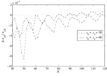
Figure 1: Relative discrepancy $\Delta n_{\mathrm{eff}}/n_{\mathrm{eff}}$ between SOB-FDFD computed and analytically calculated mode indices of step-index fiber (radius $R$ = 2 $\mu$m, material index 1.45) in air background at 1.45 $\mu$m, with increasing the number of grid points $N$ per domain width.

5 A new way to construct PMLs

An interesting question is how arbitrary the transform function in (5) is. Indeed, one may use, e.g., hyperbolic tangent for the mapping; such choice would lead to only slight changes in (6), (7), with $\cos^{2}(u\pi/2)$ etc. on $(-1,1)$ substituted by $1-u^{2}$ on the same domain. And indeed, numeric simulations in $\tanh$-transformed coordinates show results similar to those in Section 4, although convergence was found poorer for the example in figure 1, probably owing to higher steepness of appropriately transformed $\epsilon$ and $\mu$ profiles near the domain boundaries which spur numerical errors at discretization.

Going a step further, one might introduce piecewise mapping functions like $u=x$ for $|x|\leq x_{1}$, $u=x_{1}+x_{2}\tanh\frac{x-x_{1}}{x_{2}}$ for $|x|>x_{1}$, where $x_{1}$ defines the interface between space region untouched by the transformation, and $x_{2}$ the width of ‘non-absorbing perfectly matched layer’. The analogy with conventional dispersive PMLs becomes even more pronounced if we put $x_{2}\propto\lambda$, which is a rather natural choice as noted in Section 3. The advantage of this ‘piecewise’ formulation over smooth arctangent or hyperbolic tangent squeezing is that within the $|x|\leq x_{1}$, $|y|\leq y_{1}$, $|z|\leq z_{1}$ region, $\epsilon$ and $\mu$ profiles are defined as on untransformed grid; the disadvantage is that they are consequently sharper near computation domain boundaries, for the domain of the same width.

The notions of ‘complex coordinate stretching’ [14] or ‘lossy mapping of space’ [15] have long been used to derive standard (lossy) PMLs, though it was not always clear what physical sense those complex-valued ‘degrees of freedom’ added by hand to spatial variables in Maxwell equations do have; in operational terms, whether complex-valued coordinates are observable. The proposed SOB technique paves the way to construct lossless PMLs with a clear geometric meaning of outer space squeezing; and if losses should be introduced (as in frequency-domain calculations of leaky modes), this can be done by adding, under the leakage irreversibility condition, an imaginary part to refractive index of surrounding medium before squeezing.

6 Conclusion

Squeezing of open boundaries is proposed as an inexpensive and, at analytic stage, rigorous alternative to standard lossy PML technique. What makes our method so attractive is its conceptual clarity: we do not surround computation window with artificial lossy media; we do not modify Maxwell equations in any way; all we do is we choose coordinate system allowed by covariant nature of Maxwell equations and suitable for calculations—and for the finite-difference or finite-element calculations on a bounded domain, a suitable system is one that has bounded coordinates. The method is more straightforward to apply in time domain; in our proof-of-principle frequency-domain simulations of guided propagation, no spurious modes confined in the regions of strongly modified $\epsilon$ and $\mu$ have been detected.

References

References

- [1] E. Lindman, “Free-space boundary conditions for the time dependent wave equation,” J. Comput. Phys., vol. 18, pp. 66–78, 1975.
- [2] R. L. Higdon, “Numerical absorbing boundary conditions for the wave equation,” Math. Comput., vol. 49, pp. 65–90, 1987.
- [3] C. M. Rappaport and L. Bahrmasel, “An absorbing boundary condition based on anechoic absorber for EM scattering computation,” J. Electromag. Waves Appl., vol. 6, pp. 1621–1634, 1992.
- [4] Z. S. Sacks, D. M. Kingsland, R. Lee, and J.-F. Lee, “A perfectly matched anisotropic absorber for use as an absorbing boundary condition,” IEEE Trans. Antennas Propagat., vol. 43, pp. 1460–1463, 1995.
- [5] J. P. Bérenger, “A perfectly matched layer for the absorption of electromagnetic waves,” J. Comput. Phys., vol. 114, pp. 185–200, 1994.
- [6] M. W. Buksas, “Implementing the perfectly matched layer absorbing boundary condition with mimetic differencing schemes,” Prog. Electromagn. Research PIER, vol. 32, pp. 383- 411, 2001.
- [7] J. A. Schouten, Tensor Analysis for Physicists (Clarendon, Oxford, 1951).
- [8] E. J. Post, Formal Structure of Electromagnetics (North-Holland, Amsterdam, 1962).
- [9] A. J. Ward and J. B. Pendry, “Refraction and geometry in Maxwell’s equations,” J. Modern Opt., vol. 43, pp. 773–793, 1996.
- [10] A. J. Ward and J. B. Pendry, “Calculating photonic Green’s functions using a nonorthogonal finite-difference time-domain method,” Phys. Rev. B, vol. 58, pp. 7252–7259, 1998.
- [11] D. M. Shyroki, “Note on transformation to general curvilinear coordinates for Maxwell’s curl equations,” arXive:physics/0307029, 2003.
- [12] D. M. Shyroki, “Exact equivalent-profile formulation for bent optical waveguides,” arXive:physics/0605002, 2006.
- [13] F. L. Teixeira and W. C. Chew, “General closed-form PML constitutive tensors to match arbitrary bianisotropic and dispersive linear media,” IEEE Microwave Guided Wave Lett., vol. 8, pp. 223–225, 1998.
- [14] W. C. Chew and W. H. Weedon, “A 3D perfectly matched medium from modified Maxwell’s equations with stretched coordinates,” Microwave Opt. Tech. Lett., vol. 7, pp. 599–604, 1994.
- [15] C. M. Rappaport, “Perfectly mathed absorbing boundary conditions based on anisotropic lossy mapping of space,” IEEE Microwave Guided Wave Lett., vol. 5, pp. 90–92, 1995.