Applicability of Modified Effective-Range Theory to positron-atom and positron-molecule scattering

Abstract

We analyze low-energy scattering of positrons on Ar atoms and N₂ molecules using Modified Effective-Range Theory (MERT) developped by O’Malley, Spruch and Rosenberg [Journal of Math. Phys. 2, 491 (1961)]. We use formulation of MERT based on exact solutions of Schrödinger equation with polarization potential rather than low-energy expansions of phase shifts into momentum series. We show that MERT describes well experimental data, provided that effective-range expansion is performed both for $s$- and $p$-wave scattering, which dominate in the considered regime of positron energies ($0.4$ - $2$ eV). We estimate the values of the $s$-wave scattering lenght and the effective range for $e^{+}$-Ar and $e^{+}$-N₂ collisions.

Electron (and positron) scattering on atoms at very low energies is dominated by polarization forces. Modified effective range theory (MERT) was developed by O’Malley, Rosenberg and Spruch OMalley ; OMalley1 for low-energy scattering of charged particles on neutral polarizable systems in general. O’Malley OMalley2 applied MERT for electron scattering on noble gases, in particular in the region of Ramsauer- Townsend minimum, using early total Ramsauer and momentum transfer Pack experimental cross sections. Haddad and O’Malley Haddad used three parameter MERT fit for s-wave phase-shift in electron-argon scattering and Ferch, Granitza and Raith Ferch - for Ramsauer minimum in methane. Higher-order terms in MERT, resulting from short-range components of polarizabitity, were introduced by Ali and Fraser Ali . MERT analysis for Ne, Ar, Kr up to 1 eV was carefully revisited by Buckman and Mitroy Buckman who used five-parameter fit for $s$-wave and $p$-wave shifts.

Applicability of MERT to low-energy positron scattering was already hypothesized in OMalley1 . However, first measurements of total cross sections for positron scattering at low energies on noble atoms come only from seventies Costello ; Kaupilla .

The most systematic data for noble atoms, extending down to 0.3 eV were done in WSU Detroit lab, using positrons from a short-lived C¹¹ radionuclid, with about 0.1 eV energy resolution Kaupilla . Those data indicated clearly a rise of the cross section in the zero energy limit in gases, like He, Ar, H₂, Kr, Xe, CO₂, see Kaupilla . Unfortunately, subsequent experiments Sueoka ; Stein used Ne²² source and thick W-vanes positron moderator, thus worsening energy resolution and not allowing to make reliable measurements below 1 eV. To gain in signal, large apertures and strong guiding magnetic fields were used, leading to underestimation of cross sections - some data showed even a fall in the limit of zero energy for highly polarizable targets, like C₆H₆ Kimura .

Only two of the most recent set-ups reached energies below 1 eV with good signal-to-noise ratio. In San Diego annihilation rates in Ar and Xe were measured, showing a steep rise below 1 eV Marler . In Trento total cross sections in Ar and N₂ were measured Karwasz1 with angular resolution better by a factor of 30 than in some previous experiments Sueoka . Both laboratories confirm the early observations from WSU Detroit on the rise of positron cross sections in the zero-energy limit. Such a rise is also predicted by ab-initio theories McEachran , see Karwasz1 for detailed comparison. A phenomenological attempt to apply MERT-like fit for low-energy cross sections in benzene and cyclohexane was done by Karwasz, Pliszka and Zecca Karwasz2 .

In the present paper we apply MERT to positron total cross sections on argon and nitrogen, using recent experimental data from Trento Karwasz1 . We use MERT model based on direct solution of Schrödinger equation with polarization potential as originally proposed by O’Malley, Spruch and Rosenberg OMalley . Differently from earlier works, for the $p$-wave phaseshift we consider not only the polarization potential but contribution from a general-type short range interaction. This allows us to extend the MERT applicability for positrons to energies above 1 eV. A clear indication on importance of $p$-wave scattering in this energy range comes from recent differential cross sections measurements in argon Sullivan . The present model introduces a second MERT parameter for the $p$-wave shift thus developing an approximation with two parameters for both $s$ and $p$-wave phaseshifts. The first parameter is to be interpreted as a scattering length and the second as an effective range. We compare our MERT model with the expansion into momentum series valid at low energies and with ab-initio theories McEachran ; Nakanishi .

Let us briefly review the effective-range expansion for $1/r^{4}$ interaction. We divide the interaction potential between charged particle and neutral atom into the long-range part: $V_{\mathrm{p}}(r)=-\alpha e^{2}/(2r^{4})$ with $\alpha$ denoting the atomic polarizability and $e$ the charge, and the short-range part: $V_{\mathrm{s}}(r)$ describing forces acting at distances comparable to the size of atoms. In the relative coordinate the motion of particles is governed by

$$\left[\frac{\partial^{2}}{\partial r^{2}}+\frac{2}{r}\frac{\partial}{\partial r}-\frac{l(l+1)}{r^{2}}+\frac{(R^{\ast})^{2}}{r^{4}}+k^{2}\right]\Psi(r)=0,$$ (1)

where $\Psi(r)$ denotes the radial wave function for $l$-th partial wave, $\hbar k$ is the relative momentum of the particles, $R^{\ast}\equiv\sqrt{\alpha e^{2}\mu/\hbar^{2}}$ denotes a typical lenght scale related with the $r^{-4}$ interaction, and $\mu$ denotes the reduced mass. In Eq. (1) we do not include $V_{\mathrm{s}}(r)$, which is replaced by appropriate boundary condition at $r\rightarrow 0$. The Schrödinger equation with polarization potential can be solved analytically Vogt ; OMalley ; Spector (see Appendix for details). At small distances ($r\ll R^{\ast}$) behavior of $\Psi(r)$ is governed by

$$\Psi(r)\stackrel{{\scriptstyle r\rightarrow 0}}{{\sim}}\sin\left(\frac{R^{\ast}}{r}+\phi\right),$$ (2)

where $\phi$ is a parameter which is determined by the short-range part of the interaction potential. For $r\gg R^{\ast}$, $\Psi(r)$ takes the form of the scattered wave

$$\Psi(r)\stackrel{{\scriptstyle r\rightarrow\infty}}{{\sim}}\frac{1}{kr}\sin({\textstyle kr-l\frac{\pi}{2}+\eta_{l}}),$$ (3)

with the phase shift $\eta_{l}$

$$\tan\eta_{l}=\frac{m^{2}-\tan\delta^{2}+B\tan\delta(m^{2}-1)}{\tan\delta(1-m^{2})+B(1-m^{2}\tan^{2}\delta)},$$ (4)

where we use similar notation as in Ref. OMalley . Here $B=\tan({\textstyle\phi+l\frac{\pi}{2}})$, $\delta=\frac{\pi}{2}(\nu-l-\frac{1}{2})$, and $m$ and $\nu$ are parameters obtained from the analytic solution of the Mathieu’s differential equation (see Appendix). To introduce effective range we expand $B$ around zero energy: $B(k)=B(0)+\frac{1}{2}R_{0}R^{\ast}k^{2}+\ldots$ OMalley . The second term can be intepreted as correction due to the finite range of the interaction, with $R_{0}$ representing the effective range.

In the zero-energy limit expansion of MERT in series of momentum $k$ is useful. In the particular case of $l=0$, $B(0)$ can be expressed in terms of $s$-wave scattering length $a_{s}$: $B(0)=-R^{\ast}/a_{s}$, and expansion of $\cot\eta_{0}$ at $k=0$ yields OMalley ; Levy

$$q\cot\eta_{0}(q)= -\frac{1}{a}+\frac{\pi}{3a^{2}}q+\frac{4}{3a}\ln\left(\frac{q}{4}\right)q^{2}+\frac{{R_{0}}^{2}}{2(R^{\ast})^{2}}q^{2}$$

$$+\left[\frac{\pi}{3}+\frac{20}{9a}-\frac{\pi}{3a^{2}}-\frac{\pi^{2}}{9a^{3}}-\frac{8}{3a}\psi({\textstyle\frac{3}{2}})\right]q^{2}$$

$$+\ldots$$ (5)

where $a=a_{s}/R^{\ast}$, $q=kR^{\ast}$ and $\psi(\frac{3}{2})$ denotes the digamma function Abramowitz . We apply similar procedure for $p$-wave. In this case, however, we expand directly $\tan\eta_{1}$ given by Eq. (4)

$$\tan\eta_{1}= \frac{\pi q^{2}}{15}+\frac{q^{3}}{9b}-\frac{83\pi q^{4}}{23625}-\frac{4}{135b}\ln\left(\frac{q}{4}\right)q^{5}-\frac{R_{1}}{18b^{2}R^{\ast}}q^{5}$$

$$+\frac{15\pi-15\pi b^{2}-148b+120b\psi(\frac{5}{2})}{2025b^{2}}q^{5}+\ldots$$ (6)

Here, $b=B(0)$ for $l=1$, and $R_{1}$ denotes the effective range for $p$-wave. For higher partial waves we retain only the lowest order term in $k$, which is sufficient to describe the scattering in the considered regime of energies

$$\tan\eta_{l}\approx-\frac{\pi q^{2}}{8(l-\frac{1}{2})(l+\frac{1}{2})(l+\frac{3}{2})},\quad l\geq 2$$ (7)

Let us turn now to positron scattering. We compare the total cross-section measured in experiment for Ar and N₂ Karwasz1 with predictions of the theoretical model based on the effective-range expansion. In our approach the effects of the short-range potential are included both for $s$- and $p$-wave giving the leading contribution to the scattering in the considered regime of energies. Thus, our model contains four unknown parameters: the scattering length $a$ and the effective range $R_{0}$ for $s$-wave, and the zero-energy contribution $b=B(0)$ and the effective range $R_{1}$ for $p$-wave. For the investigated regime of positrons energies, $q=kR^{\ast}$ can take values larger than unity, therefore for $s$- and $p$-wave we do not use expansions (5)-(6) valid for $q\lesssim 1$, but we rather applied the initial formula (4) for the phase shift, performing only finite-range expansion for the parameter $B$. In this case, values of $\nu$ and $m$ has to be evaluated numerically, using the approach described in the Appendix.

For the calculations we use recent experimental values of the polarizability: $\alpha=11.23{a_{0}}^{3}$ and $\alpha=11.54{a_{0}}^{3}$ (atomic units), for Ar and N₂, respectively Olney . Table 1 contains values of the characteristic distance $R^{\ast}$ and the characteristic energy $E^{\ast}=\hbar^{2}/(2\mu{R^{\ast}}^{2})$ for the polarization potential, and the values of four parameters: $a$, $b$, $R_{0}$, $R_{1}$ which were determined by fitting our model to the experimental data.

In the case of N₂ the size of the molecule scaled by $R^{\ast}$ is much larger than for Ar, therefore we restricted our effective-range analysis to lower energies, fitting the model to experimental data with $E\lesssim 0.8E^{\ast}$. In this regime the contribution of the effective-range correction in $p$-wave is rather small, and one does not get reliable results for this parameter from the fitting procedure. Thus, for N₂ we considered only three parameters $a$, $b$ and $R_{0}$ accounting for effects of the short-range part of the potential.

Fig. 1 shows the experimental data for the total scattering cross-section for Ar as a function of positron collision energy. They are compared with: the MERT theoretical curve which best fits the experimental data, its low-energy expansion given by Eqs. (5)-(7), and the results of McEachran et al. McEachran . The total cross-section is presented in units of $R^{\ast}$, while the energy is scaled by $E^{\ast}$. In the inset we additionally present contributions of the $s$ and $p$ waves to the total scattering cross-section. Similar results but for the scattering of positrons on N₂ are illustrated in Fig. 2.

We note the good agreement between our model and the results of McEachran et al. McEachran at low energies. Obtained value of the scattering lenght $a_{\mathrm{s}}=-5.58a_{0}$ agrees well with the calculations of McEachran et al. McEachran ($-5.30a_{0}$), and Nakanishi and Schrader Nakanishi ($-5.09a_{0}$). A somewhat worse agreement in N₂ can partially result from poorer statistics of experimental data. Also ab-initio theoretical calculation in N₂ show a big spread in determination of $a_{s}$, see for instance Gianturco . Both for Ar and N₂ the model shows importance of $p$-wave scattering above 0.7-0.8 eV. The $s$-wave effective range for Ar amounts to $1.06a_{0}$ while in N₂ to $2.78a_{0}$ . We recall the ”size” of the N₂ molecule by the experimental determination of the maximum HOMO density along the molecule axis which is about $2.3a_{0}$ Itatani . Finally from Figs. 1 and 2 we observe that expansion into momentum series (5)-(7) works only at very low energies below $0.1$eV.

	$R^{\ast}$($a_{0}$)	$E^{\ast}$(eV)	$a_{\mathrm{s}}/R^{\ast}$	$b$	$R_{0}/R^{\ast}$	$R_{1}/R^{\ast}$
Ar	3.351	1.211	-1.665	-5.138	0.3165	2.281
N2	3.397	1.179	-2.729	-12.65	0.8186	—

Table 1: Characteristic distance $R^{\ast}$, characteristic energy $E^{\ast}$ and four fitting parameters: $a_{\mathrm{s}}$ ($s$-wave scattering length), $R_{0}$ ($s$-wave effective range), $b$ (zero-energy contribution B(0) for $p$-wave) and $R_{1}$ ($p$-wave effective range) for Ar and N₂.

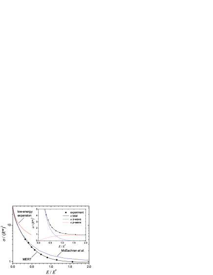
Figure 1: Total cross-section for the scattering of positrons on argon versus the energy. Depicted are: experimental data (squares), the theoretical fit based on effective-range expansion (solid line), its low-energy part given by Eqs. (5)-(7), and the theoretical results of McEachran et al. (dashed line). The inset shows in addition the $s$- and $p$-wave cross-sections. Data are scaled by the the characteristic distance $R^{\ast}$ and the characteristic energy $E^{\ast}$ of the polarization potential.

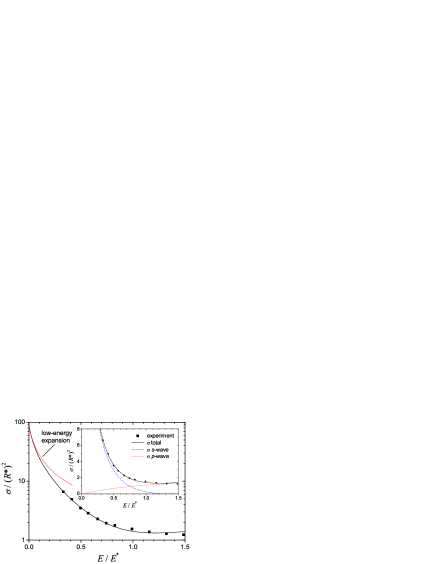
Figure 2: The same as Fig. 1 but for the scattering of positrons on N₂.

In conclusion, we performed MERT analysis using analytical solution of Schrödinger equation for polarization potential and we apply it to positron Ar (and N₂) scattering up to 2eV. The scattering length in Ar agrees well with other predictions and the effective range (for $s$-wave) is $1.06a_{0}$. More experiments are needed at low energies to validate better the effective range parameters.

Appendix A

To solve radial Schrödinger equation (1) we substitute $r=\sqrt{R^{\ast}}e^{-z}/\sqrt{k}$ and $\Psi(r)=\psi(r)\sqrt{R^{\ast}/r}$, which yields the Mathieu’s modified differential equation Erdelyi ; Abramowitz

$$\frac{d^{2}\psi}{dz^{2}}-\left[a-2q\cosh 2z\right]\psi=0.$$ (8)

where $a=(l+{\textstyle\frac{1}{2}})^{2}$ and $q=kR^{\ast}$. Two linearly indepent solutions $M(z)$ and $T(z)$ can be expressed in the following form Erdelyi ; Spector

$$M_{\nu}(z) = \sum_{n=-\infty}^{\infty}(-1)^{n}c_{n}(\nu)J_{2n+\nu}(2\sqrt{q}\cosh z),$$ (9)

$$T_{\nu}(z) = \sum_{n=-\infty}^{\infty}(-1)^{n}c_{n}(\nu)Y_{2n+\nu}(2\sqrt{q}\cosh z),$$ (10)

which defines them for $z>0$. Here, $\nu$ denotes the characteristic exponent, and $J_{\nu}(z)$ and $Y_{\nu}(z)$ are Bessel and Neumann functions respectively. Substituting the ansatz (9) and (10) into (8) one obtains the recurrence relation:

$$\left[(2n+\nu)^{2}-a\right]c_{n}+q(c_{n-1}+c_{n+1})=0,$$ (11)

which can be solved in terms of continued fractions. To this end we introduce $h_{n}^{+}=c_{n}/c_{n-1}$ and $h_{n}^{-}=c_{-n}/c_{-n+1}$ for $n>0$, which substituted into (11) gives the continued fractions $h^{+}_{n}=-q/(qh^{+}_{n+1}+d_{n})$, and $h^{+}_{n}=-q/(qh^{+}_{n+1}+d_{n})$ with $d_{n}=(2n+\nu)^{2}-a$. In practice to find numerical values of the coefficients $c_{n}$ we set $h^{+}_{m}=0$ and $h^{-}_{m}=0$ for some, sufficiently large $m$ and calculate $h^{+}_{n}$ and $h^{-}_{n}$ up to $n=1$. Characteristic exponent has to determined from Eq. (11) with $n=0$.

Asymptotic behavior of $M_{\nu}(z)$ and $T_{\nu}(z)$ for large $z$ follow immediately from asymptotic expansion of Bessel functions

$$M_{\nu}(z)\stackrel{{\scriptstyle z\rightarrow\infty}}{{\longrightarrow}} \sqrt{\frac{2}{\pi}}\frac{e^{-z/2}}{q^{1/4}}s_{\nu}\cos\left({\textstyle e^{z}\sqrt{q}-\frac{\pi}{2}\nu-\frac{\pi}{4}}\right)$$ (12)

$$T_{\nu}(z)\stackrel{{\scriptstyle z\rightarrow\infty}}{{\longrightarrow}} \sqrt{\frac{2}{\pi}}\frac{e^{-z/2}}{q^{1/4}}s_{\nu}\sin\left({\textstyle e^{z}\sqrt{q}-\frac{\pi}{2}\nu-\frac{\pi}{4}}\right)$$ (13)

where $s_{\nu}=\sum_{n=-\infty}^{\infty}c_{n}(\nu)$. To obtain asymptotic behavior for large and negative $z$ one has to join solutions $M_{\nu}(z)$ and $T_{\nu}(z)$, with another pair of solution $M_{\nu}(-z)$ and $T_{\nu}(-z)$ at $z=0$ Spector . This yields

$$M_{\nu}(z)\stackrel{{\scriptstyle z\rightarrow-\infty}}{{\longrightarrow}} \sqrt{\frac{2}{\pi}}\frac{e^{z/2}}{q^{1/4}}ms_{\nu}\cos\left({\textstyle\sqrt{q}e^{-z}+\frac{\pi}{2}\nu-\frac{\pi}{4}}\right)$$ (14)

$$T_{\nu}(z)\stackrel{{\scriptstyle z\rightarrow-\infty}}{{\longrightarrow}} -\sqrt{\frac{2}{\pi}}\frac{e^{z/2}}{q^{1/4}}\frac{s_{\nu}}{m}\Big{[}\sin\left({\textstyle\sqrt{q}e^{-z}+\frac{\pi}{2}\nu-\frac{\pi}{4}}\right)$$

$$-\cot\pi\nu(m^{2}-1)\cos\left({\textstyle\sqrt{q}e^{-z}+\frac{\pi}{2}\nu-\frac{\pi}{4}}\right)\Big{]}$$ (15)

where $m=\lim_{z\rightarrow 0^{+}}M_{\nu}(z)/M_{-\nu}(z)$.

Finally we write the wave function $\Psi(r)$ in the form

$$\Psi(r)= \sin({\textstyle\phi+\frac{\pi}{2}\nu+\frac{\pi}{4}})\sqrt{\frac{R^{\ast}}{r}}M_{\nu}\left(\ln\frac{\sqrt{R^{\ast}}}{\sqrt{k}r}\right)$$

$$+\cos({\textstyle\phi+\frac{\pi}{2}\nu+\frac{\pi}{4}})\sqrt{\frac{R^{\ast}}{r}}T_{\nu}\left(\ln\frac{\sqrt{R^{\ast}}}{\sqrt{k}r}\right),$$ (16)

where $\phi$ is a parameter which appear in the small $r$ expansion (2). Now, the behavior of $\Psi(r)$ at small and large distance described by Eqs. (2)-(4), can be readily obtained from asymptotic expansions (12)-(15).

References

- (1) T.F. O’Malley, L. Spruch, and L. Rosenberg, J. Math. Phys. 2, 491 (1961).
- (2) T.F. O’Malley, L. Rosenberg, and L. Spruch, Phys. Rev. 125, 1300 (1962).
- (3) T.F. O’Malley, Phys. Rev. 130, 1020 (1963).
- (4) C. Ramsauer and Kollath, Ann. Phys. (Lepizig) 3, 536 (1929).
- (5) J. L. Pack and A. V. Phelps, Phys. Rev. 121, 798 (1961).
- (6) G. N. Haddad and T. F. O’Malley. Austr. J. Phys. 35, 35 (1982); T. F. O’Malley and R. W. Crompton, J. Phys. B: Atom. Molec. Phys. 13, 3451 (1980).
- (7) J. Ferch. G. Granitza, and W. Raith, J. Phys. At. Mol. Phys. B 18, L445 (1985).
- (8) M. K. Ali and P. A. Fraser, J. Phys. B: Atom. Molec. Phys. 10, 3091 (1977).
- (9) S. J. Buckman and J. Mitroy, J. Phys. At. Mol. Phys. 22, 1365 (1989).
- (10) D.G. Costello, D.E. Groce, D.F. Herring and J. Wm. McGowan , Can. J.Phys. 50 (1972) 23.
- (11) W. E. Kauppila, T. S. Stein. and G. Jesion, Phys. Rev. Lett. 36, 580 (1976); see also W. E. Kauppila and S. T. Stein, Adv. At. Mol. Phys. 26, 1 (1990).
- (12) O. Sueoka and S. Mori, J. Phys. Soc. Jap. 53, 2491 (1984).
- (13) T. S. Stein, W. E. Kauppila, C. K. Kwan, S. P. Parikh, and S. Zhou, Hyperfine Inter. 73, 53 (1992).
- (14) M. Kimura, C. Makochekanwa, and O. Sueoka, J.Phys. B: At. Mol. Opt. Phys. 37, 1461.
- (15) J. P. Marler, L. D. Barnes, S. J. Gilbert, J. P. Sullivan, J. A. Young, and C. M. Surko, Nucl. Instr. Meth. Phys. Res. B 221, 84 (2004).
- (16) G. P. Karwasz, D. Pliszka, and R. S. Brusa, Nucl. Instr. Meth. B, in press, see also G. P. Karwasz, Eur. Phys. J. D 35, 267 (2005).
- (17) R.P. McEachran, A.G. Ryman and A.D. Stauffer, J. Phys. B: Atom. Molec. Phys. 12, 1031 (1979).
- (18) G. Karwasz, D. Pliszka, and A. Zecca, Proc. of SPIE Vol. 5849, 243 (2005), SPIE, Bellingham, WA.
- (19) J. P. Sullivan, S. J. Gilbert, J. P. Marler, R. G. Greaves, S. J. Buckman, and C. M. Surko, Phys. Rev. A 66, 042708 (2002).
- (20) H. Nakanishi and D.M. Schrader, Phys. Rev. A 34, 1823 (1986).
- (21) E. Vogt, and G.H. Wannier, Phys Rev. 95, 1190 (1954).
- (22) R.M. Spector, J. Math. Phys. 5, 1185 (1964).
- (23) B.R. Levy, J.B. Keller, J. Math. Phys. 4, 54 (1963).
- (24) M. Abramowitz, and I.A. Stegun Handbook of Mathematical Functions (Dover, New York, 1972).
- (25) T.N. Olney, N.M. Cann, G. Cooper and C.E. Brion, Chem. Phys. 223, 59 (1997).
- (26) F. A. Gianturco, P. Paioletti, and J. A. Rodriguez-Ruiz, Z. Phys. D 36, 51 (1996).
- (27) J. Itatani, J. Levesue, D. Zeidler, Hiromichi Niikura, H. P pin, J.C. Kieffer, P.B. Korkum and D.M. Villeneuve, Nature 432, 867 (2004).
- (28) A. Erdélyi Higher transcendental functions, Vol. III (McGraw-Hill, New York, 1955).