Excitation of surface dipole and solenoidal modes
on toroidal structures

Abstract

The time dependent Schrödinger equation inclusive of curvature effects is developed for a spinless electron constrained to motion on a toroidal surface and subjected to circularly polarized and linearly polarized waves in the microwave regime. A basis set expansion is used to determine the character of the surface currents as the system is driven at a particular resonance frequency. Surface current densities and magnetic moments corresponding to those currents are calculated. It is shown that the currents can yield magnetic moments large not only along the toroidal symmetry axis, but along directions tangential and normal to the toroidal surface as well.

1 Introduction

The control of a nanostructure’s state through electromagnetic interactions is of fundamental and practical interest Shapiro and Brumer (2003); Borzi et al. (2002); Potz (1998); Qin et al. (2003); Oosterkamp et al. (1998). Considerable effort has been directed towards the study of flat quantum rings, which, because of their topology, give rise to Aharanov-Bohm and persistent current effects Bulaev et al. (2004); Climente et al. (2005); Tian and Datta (1994); Filikhin et al. (2004); Heinzel et al. (2001); Georgiev and Geller (2004); Gylfadottir et al. (2005); Ivanov and Lobanova (2003); Latil et al. (2003); Pershin and Piermarocchi (2005a, b); Sasaki et al. (2004); Sasaki and Kawazoe (2004); Simonin et al. (2004); Viefers et al. . Currents generated on a ring are restricted to yield magnetic moments perpendicular to the plane of the ring; however, it is conceivable that structures with different topologies are capable of producing magnetic moments in different directions, a feature potentially useful when such structures are employed as nano-device elements. In this work, a toroidal structure in the presence of an electromagnetic wave on the microwave scale is considered. In contrast to rings, it is possible to excite modes for which currents circulate around the minor radius of the toroidal surface $T^{2}$ (called in what follows $``$solenoidal modes” since the focus will be on magnetic moments) in addition to the modes in which currents circulate azimuthally around the major radius ($``$dipole modes”).

The approach adopted here will be to develop

$$H=H_{0}+V(t)$$ (1)

with $H_{0}$ the Hamiltonian for a spinless electron constrained to motion on $T^{2}$ inclusive of surface curvature effects Encinosa and L.Mott (2003), and $V(t)$ the time dependent electromagnetic interaction with the form appropriate to circularly and linearly polarized microwaves propagating along the symmetry axis of the torus (here the z-axis) at a particular resonant frequency of the system. It has been shown that for the case of no external vector potential, it is possible to treat the normal degree of freedom as a spectator variable Encinosa et al. (2005). However, inclusion of a vector potential $\mathbf{A}$ with components normal to the surface complicates the situation. Reducing the full three-dimensional problem to a two-dimensional effective model serves to simplify matters considerably. The resulting Schrödinger equation is then solved with standard methods by taking ($\hbar$ = 1)

$$\Psi(t)=\sum_{n\nu}d_{n\nu}(t)\chi_{n}(\theta){\rm exp}[i\nu\phi]{\rm exp}[-iE_{n\nu}t]$$ (2)

with the $\chi_{n}(\theta){\rm exp}[-i\nu\phi]{\rm exp}[-iE_{n\nu}t]$ eigenstates of $H_{0}$. Surface current densities (SCDs) are determined and magnetic moments are calculated, from which it is shown that is it possible to selectively generate dominant oscillatory magnetic moments in different directions depending on the character of the applied signal.

The remainder of this paper is organized as follows: in section 2 the Hamiltonian on $T^{2}$ is developed by beginning with a three dimensional formulation and proceeding to restrict the particle (accounting for curvature)to $T^{2}$. In section 3 the eigenstates of $H_{0}$ that comprise the basis set are given and the solution method detailed. Section 4 presents results in the form of plots of time dependent SCDs and magnetic moments. Section 5 is reserved for conclusions.

2 The system Hamiltonian

This section presents a derivation of $H(t)$ inclusive of surface curvature (SC) effects. The necessity of accounting for SC has been shown elsewhere Encinosa et al. (2005). The central idea is upon restricting a particle in the neighborhood of a surface to the surface proper, a geometric potential $V_{C}$ is necessary to capture the full three dimensional spectra and wave functions with good fidelity.

In this work, $V_{C}$ will not be the only geometric potential. The normal component of $\mathbf{A}$ also couples to SC Pershin and Piermarocchi (2005b); Encinosa (2006). It should also be noted that in general, the Laplacian on the surface must be modified due to curvature. In the case of $T^{2}$ the symmetry of the system precludes such modifications Encinosa and L.Mott (2003).

The Schrödinger equation for a spinless electron in the presence of a vector potential ${\mathbf{A}}(t)$ (reinserting $\hbar$) is

$$H={1\over{2m}}\bigg{(}{\hbar\over i}\nabla+e{\mathbf{A}}(t)\bigg{)}^{2}\Psi=i\hbar{\partial\Psi\over\partial t}.$$ (3)

To derive the gradient appearing in Eq. (3), let ${\mathbf{e}}_{\rho},{\mathbf{e}}_{\phi},{\mathbf{e}}_{z}$ be unit vectors in a cylindrical coordinate system. Points in the neighborhood of a toroidal surface of major radius $R$ and minor radius $a$ may then be parameterized by

$$\mathbf{x}(\theta,\phi,q)=(R+a\ {\rm cos}\theta){\mathbf{e}}_{\rho}+a\ {\rm sin}\theta{\mathbf{e}}_{z}+q{\mathbf{e}}_{n}$$ (4)

with ${\mathbf{e}}_{n}$(to be given momentarily) everywhere normal to $T^{2}$, and $q$ the coordinate measuring the distance from $T^{2}$ along ${\mathbf{e}}_{n}$. The differential line element $d\mathbf{x}$ is then

$$d\mathbf{x}=a(1+k_{1}q){\mathbf{e}}_{\theta}d\theta+W(\theta,q)(1+k_{2}q){\mathbf{e}}_{\phi}d\phi+{\mathbf{e}}_{n}dq$$ (5)

with

$${\mathbf{e}}_{n}=\rm cos\theta{\mathbf{e}}_{\rho}+\rm sin\theta{\mathbf{e}}_{z}$$ (6)

$${\mathbf{e}}_{\theta}=-\rm sin\theta{\mathbf{e}}_{\rho}+\rm cos\theta{\mathbf{e}}_{z}$$ (7)

$$W(\theta,q)=R+(a+q)\rm cos\theta$$ (8)

and the toroidal principle curvatures

$$k_{1}={1\over a}$$ (9)

$$k_{2}={{\rm cos}\theta\over W(\theta,0)}.$$ (10)

The result for $\nabla$ is then

$$\nabla={\mathbf{e}}_{\theta}{1\over(a+q)}{\partial\over\partial\theta}+{\mathbf{e}}_{\phi}{1\over W(\theta,q)}{\partial\over\partial\phi}+{\mathbf{e}}_{n}{\partial\over\partial q}.$$ (11)

To proceed with the development of $H(t)$ specific choices must be made for ${\mathbf{A}}(t)$. Here the vector potential corresponding to a CPW

$${\mathbf{A}}(t)={E_{0}\over\omega}\big{[}-{\rm sin}(kz-\omega t){\mathbf{i}}+{\rm cos}(kz-\omega t){\mathbf{j}}\big{]}$$ (12)

with $E_{0}$ the field amplitude, $\omega$ the frequency and $z=(a+q)\rm sin\theta$ is taken. The LPW case can be obtained trivially from Eq. (12).

The procedure by which $V_{C}$ is obtained from Eqs. (3)-(11) is well known (more detailed derivations can be found in Burgess and Jensen (1993); Jensen and Koppe (1971); da Costa (1981, 1982); Matusani (1991); Goldstone and Jaffe (1991); Exner and Seba (1989); Schuster and Jaffe (2003)) and is summarized briefly below.

Begin by making a product ansatz for the surface and normal parts of the wave function

$$\Psi(\theta,\phi,q)\rightarrow{\chi_{S}(\theta,\phi)\chi_{N}(q)\over(1+2qh(\theta)+q^{2}k(\theta))^{1\over 2}}$$ (13)

with $h(\theta),k(\theta)$ the mean and Gaussian curvatures of the surface Kuhnel (1999), and imposing conservation of the norm through

$$|\Psi(\theta,\phi,q)|^{2}(1+2qh(\theta)+q^{2}k(\theta))d\Sigma dq\rightarrow|\chi_{S}(\theta,\phi)|^{2}|\chi_{N}(q)|^{2}d\Sigma dq$$ (14)

with $d\Sigma$ the differential surface area. The Laplacian appearing in Eq. (3) takes the form (the subscript on the gradient operator indicates only surface terms are involved)

$$\nabla^{2}=\nabla_{S}^{2}+2h(\theta){\partial\over\partial q}+{\partial^{2}\over\partial q^{2}}$$ (15)

with $q$ appearing in $\nabla_{S}^{2}$ as a parameter that can be immediately set to zero. The differentiations in Eq. (15) act upon the wave function given in Eq. (13) to yield

$$2h{\partial\over\partial q}+{\partial^{2}\over\partial q^{2}}\rightarrow{\partial^{2}\over\partial q^{2}}+h^{2}(\theta)-k(\theta)$$ (16)

in the $q\rightarrow 0$ limit. The $h^{2}(\theta)-k(\theta)$ term above is proportional to $V_{C}(\theta)$, and along with $V_{N}(q)$, the remaining $q$ differentiations can produce solutions confined arbitrarily close to a thin layer near the surface $\Sigma$.

As noted earlier, in addition to $V_{C}$ there is a second geometric potential that arises from the normal part of the ${\mathbf{A}}\cdot\nabla$ term in Eq. (3). Because any effective potential on $\Sigma$ should only involve surface variables the operator $A_{N}(\theta,\phi,q){\partial\over\partial q}$ must be addressed. One prescription to deal with this operator has been given in Pershin and Piermarocchi (2005b) and another in Encinosa (2006) which is chosen here. Begin by noting that the energy level spacing corresponding to the eigenvalues for the $\chi_{N}(q)$ normal term is large compared to surface eigenvalues so it is safe to assume there is negligible mixing among the $\chi_{N}(q)$ (this assumption was shown to be a reasonable one in Encinosa et al. (2005)). Let $G=1+2qh(\theta)+q^{2}k(\theta)$ and proceed to integrate out any $q$-dependence by writing

$$I=\int_{0}^{L}{\chi_{N}(q)\over G^{1/2}}A_{N}(\theta,\phi,q)\bigg{[}{\partial\over\partial q}{\chi_{N}(q)\over G^{1/2}}\bigg{]}Gdq$$ (17)

Given any well behaved $A_{N}$ it is simple to establish after an integration by parts that the resulting effective potential $V^{mag}$ is (with constants appended)

$$V^{mag}_{N}(\theta,\phi)={ie\hbar\over m}\bigg{[}h(\theta)A_{N}(\theta,\phi,0)+{1\over 2}{\partial A_{N}(\theta,\phi,q)\over\partial q}\bigg{|}_{q=0}\bigg{]}.$$ (18)

The ensuing Schrödinger equation can put into dimensionless form by defining

$$\alpha=a/R$$

$$F(\theta)=1+\rm\alpha\ cos\theta$$

$$\gamma_{N}={\pi\hbar\over e}$$

after which $H_{0}$ may be written

$$H_{0}={\partial^{2}\over\partial^{2}\theta}-{\alpha\ {\rm sin}\ \theta\over F(\theta)}{\partial\over\partial\theta}+{\alpha^{2}\over F^{2}(\theta)}{\partial^{2}\over\partial^{2}\phi}+h^{2}(\theta)-k(\theta).$$ (19)

The interaction potential $V(t)$ with $V^{mag}$ included becomes

$$V(t)={2i\alpha^{2}a_{T}E_{0}\over\gamma_{N}\omega}\bigg{[}{\rm sin\theta}({\rm sin\Omega cos\phi-cos\Omega sin\phi}){1\over a}{\partial\over\partial\theta}+$$

$${1\over F(\theta)}{\rm(sin\Omega sin\phi+cos\Omega\cos\phi)}{1\over R}{\partial\over\partial\phi}$$

$$-{1+2\alpha{\rm cos}\theta\over 2aF(\theta)}\tilde{A_{N}}(\theta,\phi)-{ka\over 4}{\rm sin}2\theta\rm(cos\Omega cos\phi+sin\Omega sin\phi)\bigg{]}$$ (20)

where

$$\tilde{A_{N}}(\theta,\phi)=\rm-sin\Omega cos\theta\cos\phi+\cos\Omega cos\theta\sin\phi,$$ (21)

$$\Omega(\theta)=ka\ {\rm sin}\theta-\omega t$$ (22)

and the $|{\mathbf{A}}(t)|^{2}$ term has been neglected.

Note that the length gauge Shapiro and Brumer (2003) is not employed here. Although implementing the gauge transformation in a curved geometry that leads to the dipole term does not involve any inherent difficulty, it is useful to report expressions for matrix elements should an extension to this problem involving ionization be desired (as would be possible for finite layer rather than ideal surface confinement), or for cases involving thin tori with minor radii on the order of a few angstroms subjected to visible laser light.

3 Basis set and method

In this work $R$ will be set to $500\AA$, a value in accordance with fabricated structures Garcia et al. (1997); Lorke et al. (2003, 2000); Zhang et al. (2003), and $\alpha=.5$, a value which serves as a compromise between smaller $\alpha$ where the solutions tend towards simple trigonometric functions and larger $\alpha$ which are less likely to be physically realistic.

The eigenstates of $H_{0}$ are found by diagonalizing $H_{0}$ with a 60 state basis set expansion. The sixty states comprise five azimuthal functions $(\nu=-2,...,2)$ multiplied by six positive and six negative $\theta$ parity Gram-Schmidt (GS) functions. The GS functions are constructed to be orthogonal over the integration measure $F(\theta)=1+\alpha\ \rm cos\theta$ Encinosa (a). The energetically lowest six states are dominated by the constant or $\rm cos\theta$ mode. To create a non-zero net current around the minor axis of the torus, some part of the wave function which behaves as $e^{in\theta}$ must appear; it is not until the seventh state (as ordered by energy) that a sine term appears which motivated the choice of the signal frequency as $\omega_{17}=\omega_{7}-\omega_{1}$. The resonance frequency $\omega_{ij}$ (in natural units) between any two levels $i$ and $j$ is numerically $3.09\times 10^{-8}\ (\beta_{j}-\beta_{i})\AA^{-1}$. The associated resonance wavelength between the first and seventh states corresponds to approximately $2\ cm$. The electric field value chosen here is approximately $10\ V/m$, a value large enough to induce effects but small enough to justify the neglect of the quadratic vector potential term in Eq. (3). The signal was applied to the structure for ten periods of the inverse resonance frequency, for a time of $2.04\times 10^{10}\tau$ units, which is equivalent to $t_{f}=.68ns$ with $\tau=3\times 10^{-11}ns$.

The matrix elements $\big{<}\bar{n}\bar{\nu}|V(t)|n\nu\big{>}$ can be evaluated analytically in terms of Bessel functions Encinosa (b). The system of seven first-ordered coupled equations is then solved for the $d_{n\nu}(t)$. Selection rules between the $\nu$ and $\bar{\nu}$ are sufficient to render the system of coupled equations relatively sparse allowing the system to be solved by standard methods.

4 Results

In this section SCDs as computed from

$$\mathbf{J}(t)={e\hbar\over m}Im\big{[}\Psi^{*}(\theta,\phi,t)\nabla_{S}\Psi(\theta,\phi,t)\big{]}$$ (23)

are found. Again, the subscript on the gradient operator indicates only surface terms are involved. From the $\mathbf{J}(t)$, magnetic moments

$$\mathbf{M}(t)={1\over 2}\int_{0}^{2\pi}\int_{0}^{2\pi}\mathbf{r}\times\mathbf{J}dA$$ (24)

with $dA=aW(\theta)d\theta d\phi$ are presented. It is possible to write $\mathbf{M}(t)$ in terms of unit vectors ${\mathbf{e}}_{\theta},{\mathbf{e}}_{\phi},{\mathbf{e}}_{n}$, but because the interest lies in comparing solenoidal to dipole modes, the components along ${\mathbf{e}}_{\rho},{\mathbf{e}}_{\phi},{\mathbf{e}}_{z}$ are shown instead. Explicit forms for the magnetic moments $M_{\rho}(t),M_{\phi}(t),M_{z}(t)$ are given in the Appendix.

Before presenting results for the currents and moments, it is worth showing representative plots of the time dependent coefficients $d_{i}(t)$. First let $L$ serve as a collective index for the values $i=1....6$. In Fig. 1, $|d_{1}(t)|^{2}$ and $|d_{7}(t)|^{2}$ for the LPW are shown, and Fig. 2 gives the same for the CPW. In both situations, $|d_{7}(t)|^{2}$ is small as compared to the remaining $|d_{L}(t)|^{2}$, but oscillate at a much slower frequency than the $|d_{L}(t)|^{2}$. As was noted previously, it is $d_{7}(t)$ that must multiply the sine terms to combine with the positive $\theta$ parity parts of the total wave function to yield currents around the minor radius, so it is the time scale of $d_{7}(t)$ that will set the time scale and magnitudes of $\mathbf{J}(t)$ and $\mathbf{M}(t)$.

Results for SCDs as functions of $\theta$ evaluated at $t_{f}$ are shown in Figs. 3 and 4 for the LPW. Fig. 3 plots $J^{a}_{\theta}(t_{f},\theta)$, the current calculated from employing only the $d_{L}(t)$, and Fig. 4 plots $J^{b}_{\theta}(t_{f},\theta)$, the current resulting from inclusion of $d_{7}(t)$ summed over the $d_{L}(t)$, both at $\phi=0$. The results illustrate that the net current resulting from $J^{a}_{\theta}(t_{f},\theta)$ is zero, but is non-zero for $J^{b}_{\theta}(t_{f},\theta)$. Figs. 5 and 6 plot the same quantities for the CPW. Results for the azimuthal current $J_{\phi}(t_{f},\phi)$ at $\theta=0$ and $\theta=\pi$ are shown in Figs. 7 for the LPW and in Fig. 8 for the CPW. The contribution from terms proportional to $d_{7}(t)$ is always much smaller than the contribution arising solely from the $d_{L}(t)$ terms, so they have not been shown separately. No net azimuthal current results from the LPW, and only a small current is present in for the CPW case.

In Fig. 9 the $M_{i}(t)$ for the LPW are shown for a duration of $t_{f}$ at $\phi=\pi/2,\theta=0$. The surprising result here is that $M_{\phi}(t)$ is generally an order of magnitude larger than the dipole moment $M_{z}(t)$. Although not shown here, it is observed that as the torus is traversed in the $\phi$ direction, the direction of the largest component of the magnetic moment is consistent with a magnetic moment perpendicular to the direction of polarization. The corresponding results for the CPW presented in Fig. 10 indicate that the dipole mode here is four orders of magnitude larger than any solenoidal modes, a result that holds true at every angle.

The above results were applicable to an ideal situation wherein the structure is situated on a surface transparent to microwaves. It is interesting to consider what is perhaps the more realistic case of the incident wave interfering with its reflected part.

In order to see whether the interference of two polarized waves propagating along the z-axis can enhance transitions to solenoidal modes, an incoming electromagnetic wave being reflected at a completely reflecting flat surface ($`$mirror’) parallel to the horizontal symmetry plane of the torus was considered. The mirror is positioned at variable distances $z_{0}$ from the central plane in order to study how superposition of the incoming and reflected linear polarized wave fronts might affect the relative amplitude of the solenoidal modes. The general arguments will be made for the CPW; the LPW results are a special case of those for the CPW.

At the mirror, the electric field must satisfy the boundary condition of no total transverse modes

$${\mathbf{E}}_{in}(z_{0},t)+{\mathbf{E}}_{out}(z_{0},t)=0,$$ (25)

The location and effect of the reflecting mirror on the incoming wave front in this context may be simply modeled in form of an additional phase $\phi_{0}=-2kz_{0}$ in the reflected field amplitude. The signs of $\omega$ and $z_{0}$ can be chosen according from the incident direction of the incoming wave. From Eq. (25), the reflected wave amplitude must be:

$${\mathbf{E}}_{out}(z,t)={E_{0}}\big{[}-{\rm cos}(kz+\omega t^{\prime}){\mathbf{i}}+{\rm sin}(kz+\omega t^{\prime}){\mathbf{j}}\big{]}$$ (26)

with $t^{\prime}=t-t_{0}$; and $t_{0}={-{2kz_{0}}/\omega}$. Thus, the reflected wave amplitude can be obtained from the incoming wave amplitude by letting

$$\omega\rightarrow-\omega,\,\,\,t\rightarrow t^{\prime},\,\,\,{\mathbf{j}}\rightarrow-{\mathbf{j}}.$$ (27)

in Eq. (26).

Several different positions for the position of the mirror plane ($z_{0}=a$, $\lambda\over 4$, $\lambda\over 2$ and $\lambda\over 8$), were investigated. The general outcome is simple oscillatory behavior with different but small amplitudes while $\big{|}d_{1}\big{|}^{2}$ stays close to 1. For $z_{0}={\lambda\over 4}$, all coefficients $d_{2},\dots,d_{7}$ are numerically nearly equal to zero, while $d_{1}$ stays constant and identical to 1. This is due to the fact that the electric field amplitude ${\mathbf{E}}$ reaches its maximum value, thus the field gradient is essentially zero over the whole torus. In all of these cases, the system stays essentially in the ground state and no transitions are observed.

The optimal mirror position that maximized the value $\big{|}d_{7}(t)\big{|}^{2}$ was determined to be at

$$z_{0}\approx 0.0027\lambda,$$ (28)

where it was found that $\big{|}d_{7}\big{|}^{2}$ reaches its maximum amplitude of roughly $7*10^{-7}$. This is an increase of up to 3 to 4 orders of magnitude for positions around $\lambda\over 4$ discussed above.

The analogous results for the interference cases to those presented above are given below. Figs. 11 and 12 show $|d_{1}(t)|^{2}$ and $|d_{7}(t)|^{2}$ plots for the LPW and CPW. It is worth noting that while the $|d_{7}(t)|^{2}$ time scale does not vary greatly due to interference as compared to the results in Figs. 1 and 2, the $|d_{1}(t)|^{2}$ time scale is very different in both cases.

The SCD plots for the LPW do not appear qualitatively different than the results already presented in Figs. 3, 4 and 7, so in the interest of conciseness those results are not presented here. However, an interesting result is shown in Fig. 13, wherein a clear signature of a circulatory $J^{b}_{\theta}(t_{f},\theta)$ SCD at $\phi=0$ is shown for the CPW due to the presence of the $d_{7}(t)$ term. Fig. 14 shows there is also a circulatory azimuthal SCD at $\theta=\pi$.

The LPW magnetic moment results are given in Fig. 15. The frequency of oscillation has again been reduced, and the overall magnitude of $M_{z}(t)$ is smaller than that of $M_{\phi}(t)$. Fig. 16 shows that for the CPW, $M_{z}(t)>M_{\phi}(t)$; this is observed to be independent of the azimuthal point at which the $M_{i}(t)$ are calculated.

5 Conclusions

This work presents a general framework for calculating surface current densities and magnetic moments on a toroidal surface in the presence of an electromagnetic wave. A proof of principle calculation demonstrating that polarized microwaves can cause circulating surface currents around the toroidal minor radius in addition to azimuthal currents was given. Rather than employ the dipole approximation, matrix elements of the electromagnetic term were evaluated in closed form. While there can be little doubt that the dipole approximation would be perfectly valid for the system considered, there are cases involving ionization or surface states with energies characterized by much smaller minor radii that warrant exact expressions.

The magnetic moments calculated in this work show that it is in principle possible to manipulate surface currents in a manner that causes the moments to $``$point” predominantly in particular directions at certain times. Our preliminary results indicate that interference due to reflection could potentially play an important role in the development of this topic.

The realization of the model problem considered here may be physically realizable with current experimental methods by placing a thin layer of a good conductor over an InAs toroidal structure. The extension of this work to metallic carbon nanotube tori is likely possible but would require some effort to account for the lattice. Preliminary work indicates that modelling the carbon sites by weak delta function potentials requires a larger basis set than employed here.

Acknowledgments

The authors would like to thank B. Etemadi for useful discussions. This work has been funded in parts by NIH Grant HD 41829 (M. Jack).

Appendix

This appendix presents closed-form expressions for the integrated magnetic moment and its components. The magnetic moment ${\bf M}(t)$ has been deferred as:

$$\mathbf{M}(t)={1\over 2}\int_{0}^{2\pi}\int_{0}^{2\pi}\mathbf{r}\times\mathbf{J}({\mathbf{r}},t)dA$$ (A.1)

with the radius vector ${\mathbf{r}}$ on the $T^{2}$ surface generated by

$${\mathbf{r}}\equiv{(R+a\cos\theta)}{{\mathbf{e}}_{\rho}}+{a\sin\theta}{{\mathbf{e}}_{z}}$$ (A.2)

and the surface gradient being

$$\nabla_{S}={{\mathbf{e}}_{\theta}}\,{1\over a}\,{{\partial}\over{\partial\theta}}+{{\mathbf{e}}_{\phi}}\,{1\over{R+a\cos\theta}}\,{{\partial}\over{\partial\phi}}.$$ (A.3)

The time dependent current density ${\mathbf{J}}({\mathbf{r}},t)$ in Eq. (A.1) is defined in Eq. (23) with the wave function $\Psi({\mathbf{r}},t)$ given in Eq. (2) as solution of the time dependent Schrödinger equation. Here express the $\theta$ dependent part of the eigenstates, $\chi_{n}(\theta)$, directly in terms of sums of cosines with coefficients $C_{n}^{k}$ for positive $\theta$ parity solutions, or as sums of sines with coefficients $D_{n}^{k}$ for negative $\theta$ parity solutions respectively:

$$\chi_{n}(\theta)=\left\{\begin{array}[]{lll}{1\over\sqrt{\pi}}\sum\limits_{k=0}^{5}C_{n}^{k}\cos(k\theta)&\textrm{for}&n=1\ldots 6;\\ {1\over\sqrt{\pi}}\sum\limits_{k=1}^{5}D_{n}^{k}\sin(k\theta)&\textrm{for}&n=7.\end{array}\right.$$ (A.4)

Now introduce the following constants $M_{0}$, $C$ and $A$:

$$M_{0}={{e\hbar}\over{4m_{e}}}R^{2};\qquad C={{e\hbar}\over{2m_{e}}};\qquad A={\pi R^{2}}.$$ (A.5)

Applying Eq. (A.2) through Eq. (A.5) the time dependent magnetic moment ${\bf M}(t)$ in Eq. (A.1) can be written as integral via the surface variables $\theta$ and $\phi$ with $F(\theta)\equiv 1+\alpha\cos\theta$:

$${\bf M}(t) = -i{\pi M_{0}}\int\limits_{0}^{2\pi}d{\phi}\int\limits_{-\pi}^{\pi}d{\theta}\Big{[}\alpha F(\theta){J_{\phi}}\,{{\mathbf{e}}_{z}}-F(\theta)(\cos\theta+\alpha){J_{\theta}}\,{{\mathbf{e}}_{\phi}}-\alpha^{2}\sin\theta{J_{\phi}}\,{{\mathbf{e}}_{\rho}}\Big{]}$$ (A.6)

with following expressions for the current densities:

$${J_{\phi}}({\mathbf{r}},t) = \Psi^{*}({\mathbf{r}},t){{\partial\Psi}\over{\partial\phi}}({\mathbf{r}},t)-\Psi({\mathbf{r}},t){{\partial\Psi^{*}}\over{\partial\phi}}({\mathbf{r}},t);$$ (A.7)

$${J_{\theta}}({\mathbf{r}},t) = \Psi^{*}({\mathbf{r}},t){{\partial\Psi}\over{\partial\theta}}({\mathbf{r}},t)-\Psi({\mathbf{r}},t){{\partial\Psi^{*}}\over{\partial\theta}}({\mathbf{r}},t).$$ (A.8)

The currents in Eq. (A.7) and Eq. (A.8) can be re-expressed as

$${J_{\phi}}({\mathbf{r}},t) = \sum\limits_{i,j}d_{i}^{*}(t)d_{j}(t)e^{i\omega_{ij}t}{J_{\phi}^{ij}}({\mathbf{r}}),$$ (A.9)

$${J_{\theta}}({\mathbf{r}},t) = \sum\limits_{i,j}d_{i}^{*}(t)d_{j}(t)e^{i\omega_{ij}t}{J_{\theta}^{ij}}({\mathbf{r}}),$$ (A.10)

with the time independent current expressions ${J_{\phi}^{ij}}(\theta,\phi)$ and ${J_{\theta}^{ij}}(\theta,\phi)$ presented in the following way ($\omega_{ij}\equiv{E_{ij}\over\hbar}\equiv{{E_{i}-E_{j}}\over\hbar}$; $\nu_{ij}\equiv\nu_{i}-\nu_{j}$):

$${J_{\phi}^{ij}}(\theta,\phi) = 2i\left(\nu_{i}+\nu_{j}\right)e^{-i\nu_{ij}\phi}\chi_{i}(\theta)\chi_{j}(\theta);$$ (A.11)

$${J_{\theta}^{ij}}(\theta,\phi) = 2e^{-i\nu_{ij}\phi}\Big{(}\chi_{i}^{*}{{\partial\chi_{j}}\over{\partial\theta}}-\chi_{j}{{\partial\chi_{i}^{*}}\over{\partial\theta}}\Big{)}.$$ (A.12)

For the final results for the magnetic moments we prepare the integrations over $\theta$ and $\phi$. The $\phi$-integration yields following three integrals:

$$\int\limits_{0}^{2\pi}d{\phi}\,e^{i(\omega_{ij}t-\nu_{ij}\phi)}{\mathbf{e}}_{z} = 2\pi\delta(\nu_{i}-\nu_{j})e^{i\omega_{ij}t}{\mathbf{e}}_{z},$$ (A.13)

$$\int\limits_{0}^{2\pi}d{\phi}\,e^{i(\omega_{ij}t-\nu_{ij}\phi)}{\mathbf{e}}_{\phi} = \pi\bigg{[}\Big{(}\delta_{p}+\delta_{n}\Big{)}{\mathbf{e}}_{y}+i\Big{(}\delta_{p}-\delta_{n}\Big{)}{\mathbf{e}}_{x}\bigg{]}e^{i\omega_{ij}t},$$ (A.14)

$$\int\limits_{0}^{2\pi}d{\phi}\,e^{i(\omega_{ij}t-\nu_{ij}\phi)}{\mathbf{e}}_{\rho} = \pi\bigg{[}\Big{(}\delta_{p}+\delta_{n}\Big{)}{\mathbf{e}}_{x}-i\Big{(}\delta_{p}-\delta_{n}\Big{)}{\mathbf{e}}_{y}\bigg{]}e^{i\omega_{ij}t},$$ (A.15)

which includes the Kroneckerdelta expressions

$$\delta_{p}\equiv\delta(\nu_{j}-\nu_{i}+1); \delta_{n}\equiv\delta(\nu_{j}-\nu_{i}-1);$$ (A.16)

$$\delta_{-}\equiv\delta(k-l); \delta_{+}\equiv\delta(k+l);$$ (A.17)

$$\delta_{-}^{\pm 1}\equiv\delta(k-l\pm 1); \delta_{+}^{\pm 1}\equiv\delta(k+l\pm 1);$$ (A.18)

$$\delta_{-}^{\pm 2}\equiv\delta(k-l\pm 2); \delta_{+}^{\pm 2}\equiv\delta(k+l\pm 2).$$ (A.19)

The final results for the $\theta$-integration are based on following integrals of products of sines and cosines:

$$\int\limits_{-\pi}^{\pi}d{\theta}\,\alpha F(\theta)\cos(k\theta)\cos(l\theta)={{\alpha}\over 2}\Bigg{[}\delta_{-}+\delta_{+}+{{\alpha}\over 2}\Big{(}\delta_{-}^{-1}+\delta_{-}^{+1}+\delta_{+}^{-1}+\delta_{+}^{+1}\Big{)}\Bigg{]};$$ (A.20)

$$\int\limits_{-\pi}^{\pi}d{\theta}\,\alpha F(\theta)\sin(k\theta)\sin(l\theta)={{\alpha}\over 2}\Bigg{[}\delta_{-}-\delta_{+}+{{\alpha}\over 2}\Big{(}\delta_{-}^{-1}+\delta_{-}^{+1}-\delta_{+}^{-1}-\delta_{+}^{+1}\Big{)}\Bigg{]};$$ (A.21)

$$\int\limits_{-\pi}^{\pi}d{\theta}\,F(\theta)(\cos\theta+\alpha)\cos(k\theta)\cos(l\theta)=$$

$$= {1\over 2}\Bigg{[}{3\over 2}\alpha\Big{(}\delta_{-}+\delta_{+}\Big{)}+{1\over 2}\Big{(}1+\alpha^{2}\Big{)}\Big{(}\delta_{-}^{-1}+\delta_{-}^{+1}+\delta_{+}^{-1}+\delta_{+}^{+1}\Big{)}+{{\alpha}\over 4}\Big{(}\delta_{-}^{-2}+\delta_{-}^{+2}+\delta_{+}^{-2}+\delta_{+}^{+2}\Big{)}\Bigg{]};$$

$$\int\limits_{-\pi}^{\pi}d{\theta}\,F(\theta)(\cos\theta+\alpha)\sin(k\theta)\sin(l\theta)=$$

$$= {1\over 2}\Bigg{[}{3\over 2}\alpha\Big{(}\delta_{-}-\delta_{+}\Big{)}+{1\over 2}\Big{(}1+\alpha^{2}\Big{)}\Big{(}\delta_{-}^{-1}+\delta_{-}^{+1}-\delta_{+}^{-1}-\delta_{+}^{+1}\Big{)}+{{\alpha}\over 4}\Big{(}\delta_{-}^{-2}+\delta_{-}^{+2}-\delta_{+}^{-2}-\delta_{+}^{+2}\Big{)}\Bigg{]};$$

$$\int\limits_{-\pi}^{\pi}d{\theta}\,\alpha^{2}\sin(\theta)\cos(k\theta)\sin(l\theta)={{\alpha^{2}}\over 4}\Big{(}\delta_{+}^{-1}-\delta_{+}^{+1}-\delta_{-}^{-1}+\delta_{-}^{+1}\Big{)}.$$ (A.24)

These results in Eq. (A.20) to (A.24) combine to the final $\theta$-integrals of products of eigenstates $\chi_{i}$, $\chi_{j}$:

$$\int\limits_{-\pi}^{\pi}d{\theta}\,\chi_{i}(\theta)\,\chi_{j}(\theta)\,F(\theta) = {{1}\over{2\pi}}\left\{\begin{array}[]{lll}\sum\limits_{k,l=0}^{5}C_{i}^{k}C_{j}^{l}\bigg{[}\delta_{-}+\delta_{+}+{{\alpha}\over 2}\Big{(}\delta_{-}^{-1}+\delta_{-}^{+1}+\delta_{+}^{-1}+\delta_{+}^{+1}\Big{)}\bigg{]}&\textrm{for}&i,j=1\ldots 6;\\ &\\ \sum\limits_{k,l=1}^{5}D_{i}^{k}D_{j}^{l}\bigg{[}\delta_{-}-\delta_{+}+{{\alpha}\over 2}\Big{(}\delta_{-}^{-1}+\delta_{-}^{+1}-\delta_{+}^{-1}-\delta_{+}^{+1}\Big{)}\bigg{]}&\textrm{for}&i=j=7;\end{array}\right.$$ (A.28)

$$\int\limits_{-\pi}^{\pi}d{\theta}\Big{(}\chi_{i}{{\partial\chi_{j}}\over{\partial\theta}}-\chi_{j}{{\partial\chi_{i}}\over{\partial\theta}}\Big{)}F(\theta)\,(\cos\theta+\alpha)=$$ (A.32)

$$= {{1}\over{2\pi}}\sum\limits_{k=0}^{5}\sum\limits_{l=1}^{5}\Bigg{\{}k\cdot\bigg{[}{3\over 2}\alpha\Big{(}\delta_{-}+\delta_{+}\Big{)}+{1\over 2}\Big{(}1+\alpha^{2}\Big{)}\Big{(}\delta_{-}^{-1}+\delta_{-}^{+1}+\delta_{+}^{-1}+\delta_{+}^{+1}\Big{)}$$

$$\qquad\qquad\qquad\quad+{{\alpha}\over 4}\Big{(}\delta_{-}^{-2}+\delta_{-}^{+2}+\delta_{+}^{-2}+\delta_{+}^{+2}\Big{)}\bigg{]}$$

$$\qquad\qquad\quad+l\cdot\bigg{[}{3\over 2}\alpha\Big{(}\delta_{-}-\delta_{+}\Big{)}+{1\over 2}\Big{(}1+\alpha^{2}\Big{)}\Big{(}\delta_{-}^{-1}+\delta_{-}^{+1}-\delta_{+}^{-1}-\delta_{+}^{+1}\Big{)}$$

$$\qquad\qquad\qquad\quad+{{\alpha}\over 4}\Big{(}\delta_{-}^{-2}+\delta_{-}^{+2}-\delta_{+}^{-2}-\delta_{+}^{+2}\Big{)}\bigg{]}\Bigg{\}}$$

$$\qquad\qquad\quad\cdot\left\{\begin{array}[]{lllll}C_{i}^{k}D_{j}^{l}&\textrm{for}&i=1\ldots 6&\textrm{and}&j=7;\\ \left(-C_{j}^{k}D_{i}^{l}\right)&\textrm{for}&i=7&\textrm{and}&j=1\ldots 6;\end{array}\right.$$

$$\int\limits_{-\pi}^{\pi}d{\theta}\chi_{i}(\theta)\,\chi_{j}(\theta)\sin\theta=$$ (A.36)

$$= {1\over{4\pi}}\sum\limits_{k=0}^{5}\sum\limits_{l=1}^{5}\Big{(}\delta_{+}^{-1}-\delta_{+}^{+1}-\delta_{-}^{-1}+\delta_{-}^{+1}\Big{)}\cdot\left\{\begin{array}[]{lllll}C_{i}^{k}D_{j}^{l}&\textrm{for}&i=1\ldots 6&\textrm{and}&j=7;\\ C_{j}^{k}D_{i}^{l}&\textrm{for}&i=7&\textrm{and}&j=1\ldots 6.\end{array}\right.$$

In the final expression for the magnetic moment ${\bf M}$, re-express ${\mathbf{e}}_{x}$ and ${\mathbf{e}}_{y}$ in terms of ${\mathbf{e}}_{\phi}$ and ${\mathbf{e}_{\rho}}$ while introducing the fixed angular variable $\phi$:

$${\mathbf{e}}_{x} = -\sin\phi\,{\mathbf{e}}_{\phi}+\cos\phi\,{\mathbf{e}}_{\rho};$$

$${\mathbf{e}}_{y} = \cos\phi\,{\mathbf{e}}_{\phi}+\sin\phi\,{\mathbf{e}}_{\rho}.$$ (A.38)

The $\theta$-integration finally yields three contributions ${\bf M}_{1}(t)$, ${\bf M}_{2}(t)$ and ${\bf M}_{3}(t)$ for the total magnetic moment. The dipole mode ${\bf M}_{1}$ ($\equiv{\bf M}_{z}$) parallel to the central symmetry axis can be determined using the definitions $d_{i}^{R}(t)\equiv\textrm{Re}\left(d_{i}(t)\right)$ and $d_{i}^{I}(t)\equiv\textrm{Im}\left(d_{i}(t)\right)$ as:

$${\bf M}_{1}(t)\equiv{\bf M}_{z}(t) = -i{\alpha\pi M_{0}}\int\limits_{0}^{2\pi}d{\phi}\int\limits_{-\pi}^{\pi}d{\theta}F(\theta){J_{\phi}}(\theta,\phi,t)\,{{\mathbf{e}}_{z}}=$$ (A.39)

$$= {\mathbf{e}}_{z}\,(4\alpha\pi M_{0})\sum\limits_{i,j=1}^{7}\left(\nu_{i}+\nu_{j}\right)\delta\left(\nu_{i}-\nu_{j}\right)$$

$$\cdot\bigg{[}\Big{(}d_{i}^{R}(t)d_{j}^{R}(t)+d_{i}^{I}(t)d_{j}^{I}(t)\Big{)}\cos(\omega_{ij}t)-\Big{(}d_{i}^{R}(t)d_{j}^{I}(t)-d_{i}^{I}(t)d_{j}^{R}(t)\Big{)}\sin(\omega_{ij}t)\bigg{]}$$

$$\int\limits_{-\pi}^{\pi}d{\theta}\,\chi_{i}(\theta)\,\chi_{j}(\theta)\,F(\theta);\qquad\qquad\qquad 4\alpha\pi M_{0}={{e\hbar}\over{2m_{e}}}(2\pi aR).$$

The two solenoidal modes are expressed by ${\bf M}_{2}(t)$ and ${\bf M}_{3}(t)$. ${\bf M}_{2}$ is proportional to the integrated current term $J_{\theta}$ in Eq. (A.8):

$${\bf M}_{2}(t) = i{\pi M_{0}}\int\limits_{0}^{2\pi}d{\phi}\int\limits_{-\pi}^{\pi}d{\theta}F(\theta)(\cos\theta+\alpha){J_{\theta}}(\theta,\phi,t)\,{{\mathbf{e}}_{\phi}}=$$ (A.40)

$$= -2\pi M_{0}\sum\limits_{i,j=1}^{7}\Bigg{\{}\bigg{[}\Big{(}d_{i}^{R}(t)d_{j}^{I}(t)-d_{i}^{I}(t)d_{j}^{R}(t)\Big{)}\Big{(}\delta_{p}\cos(\omega_{ij}t-\phi)+\delta_{n}\cos(\omega_{ij}t+\phi)\Big{)}$$

$$\qquad\qquad+\Big{(}d_{i}^{R}(t)d_{j}^{R}(t)+d_{i}^{I}(t)d_{j}^{I}(t)\Big{)}\Big{(}\delta_{p}\sin(\omega_{ij}t-\phi)+\delta_{n}\sin(\omega_{ij}t+\phi)\Big{)}\bigg{]}{\mathbf{e}}_{\phi}$$

$$\qquad\qquad+\bigg{[}\Big{(}d_{i}^{R}(t)d_{j}^{I}(t)-d_{i}^{I}(t)d_{j}^{R}(t)\Big{)}\Big{(}\delta_{p}\sin(\omega_{ij}t-\phi)-\delta_{n}\sin(\omega_{ij}t+\phi)\Big{)}$$

$$\qquad\qquad+\Big{(}d_{i}^{R}(t)d_{j}^{R}(t)+d_{i}^{I}(t)d_{j}^{I}(t)\Big{)}\Big{(}\delta_{p}\cos(\omega_{ij}t-\phi)-\delta_{n}\cos(\omega_{ij}t+\phi)\Big{)}\bigg{]}{\mathbf{e}}_{\rho}\Bigg{\}}$$

$$\qquad\qquad\cdot\int\limits_{-\pi}^{\pi}d{\theta}\Big{(}\chi_{i}{{\partial\chi_{j}}\over{\partial\theta}}-\chi_{j}{{\partial\chi_{i}}\over{\partial\theta}}\Big{)}F(\theta)\,(\cos\theta+\alpha);\quad 2\pi M_{0}={{e\hbar}\over{2m_{e}}}(\pi R^{2}).$$

The second solenoidal mode ${\bf M}_{3}$ is proportional to the integrated current $J_{\phi}$ in Eq. (A.7):

$${\bf M}_{3}(t)=i{\alpha^{2}\pi M_{0}}\int\limits_{0}^{2\pi}d{\phi}\int\limits_{-\pi}^{\pi}d{\theta}\sin\theta{J_{\phi}}(\theta,\phi,t)\,{{\mathbf{e}}_{\rho}}=$$ (A.41)

$$= -4{\alpha^{2}}\pi M_{0}\sum\limits_{i,j=1}^{7}{\left(\nu_{i}+\nu_{j}\right)\over 2}\Bigg{\{}\bigg{[}\Big{(}d_{i}^{R}(t)d_{j}^{I}(t)-d_{i}^{I}(t)d_{j}^{R}(t)\Big{)}\Big{(}\delta_{p}\cos(\omega_{ij}t-\phi)-\delta_{n}\cos(\omega_{ij}t+\phi)\Big{)}$$

$$\qquad\qquad\qquad\qquad+\Big{(}d_{i}^{R}(t)d_{j}^{R}(t)+d_{i}^{I}(t)d_{j}^{I}(t)\Big{)}\Big{(}\delta_{p}\sin(\omega_{ij}t-\phi)-\delta_{n}\sin(\omega_{ij}t+\phi)\Big{)}\bigg{]}{\mathbf{e}}_{\phi}$$

$$\qquad\qquad\qquad\qquad+\bigg{[}-\Big{(}d_{i}^{R}(t)d_{j}^{I}(t)-d_{i}^{I}(t)d_{j}^{R}(t)\Big{)}\Big{(}\delta_{p}\sin(\omega_{ij}t-\phi)+\delta_{n}\sin(\omega_{ij}t+\phi)\Big{)}$$

$$\qquad\qquad\qquad\qquad+\Big{(}d_{i}^{R}(t)d_{j}^{R}(t)+d_{i}^{I}(t)d_{j}^{I}(t)\Big{)}\Big{(}\delta_{p}\cos(\omega_{ij}t-\phi)+\delta_{n}\cos(\omega_{ij}t+\phi)\Big{)}\bigg{]}{\mathbf{e}}_{\rho}\Bigg{\}}$$

$$\qquad\qquad\qquad\qquad\cdot\int\limits_{-\pi}^{\pi}d{\theta}\,\chi_{i}(\theta)\,\chi_{j}(\theta)\sin\theta;\qquad\qquad\qquad 2{\alpha^{2}}\pi M_{0}={{e\hbar}\over{2m_{e}}}\left(\pi a^{2}\right).$$

The two components mentioned in the text, $M_{\rho}(t)$ and $M_{\phi}(t)$, can then be very easily obtained from Eq. (A.30) and (A.31) by adding ${\bf M}_{2}$ and ${\bf M}_{3}$ and projecting into the directions ${\mathbf{e}}_{\rho}$ or ${\mathbf{e}}_{\phi}$.

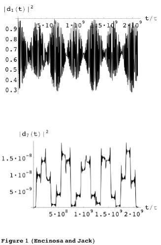
FIG 1. : Ground state $|d_{1}(t)|^{2}$ and seventh state $|d_{7}(t)|^{2}$ probability amplitudes for the system subjected to a LPW along the toroidal symmetry axis (time scale here: $\tau=3\times 10^{-11}\,ns$).

FIG 2. : Ground state $|d_{1}(t)|^{2}$ and seventh state $|d_{7}(t)|^{2}$ probability amplitudes for the system subjected to a CPW along the toroidal symmetry axis.

FIG 3. : $J^{a}_{\theta}(t_{f},\theta)$ in units of $J_{0}=e\hbar/m$ (longest arrow = $.00015$) plotted on the torus (in units of $R=1$) at $\phi=0$ in $\theta=\pi/4$ intervals for the LPW case. The net current integrated over the loop is zero ($t_{f}=0.68ns$).

FIG 4. : $J^{b}_{\theta}(t_{f},\theta)$ plotted on the torus (in units of $R=1$) at $\phi=0$ in $\theta=\pi/4$ intervals for the LPW case. The longest arrow is $3\times 10^{-6}J_{0}$. The net current integrated over the loop is non-zero and arises from the presence of the negative $\theta$ parity $d_{7}(t)$ amplitude.

FIG 5. : $J^{a}_{\theta}(t_{f},\theta)$ plotted on the torus (in units of $R=1$) at $\phi=0$ in $\theta=\pi/4$ intervals for the CPW case. The longest arrow is $.034\times 10^{-6}J_{0}$. The net current integrated over the loop is zero.

FIG 6. : $J^{b}_{\theta}(t_{f},\theta)$ plotted on the torus (in units of $R=1$) at $\phi=0$ in $\theta=\pi/4$ intervals for the CPW case. The longest arrow is $6.2\times 10^{-7}J_{0}$. The net current integrated over the loop is small, but non-zero.

FIG 7. : $J_{\phi}(t_{f},\phi)$ plotted on the torus (in units of $R=1$) at $\theta=0$ in $\phi=\pi/2$ intervals for the LPW case. The longest arrow is $.011J_{0}$. The net current integrated over the loop is zero.

FIG 8. : $J_{\phi}(t_{f},\phi)$ plotted on the torus (in units of $R=1$) at $\theta=0$ in $\phi=\pi/2$ intervals for the CPW case. The net current integrated over the loop is non-zero. The longest arrow is $.11J_{0}$.

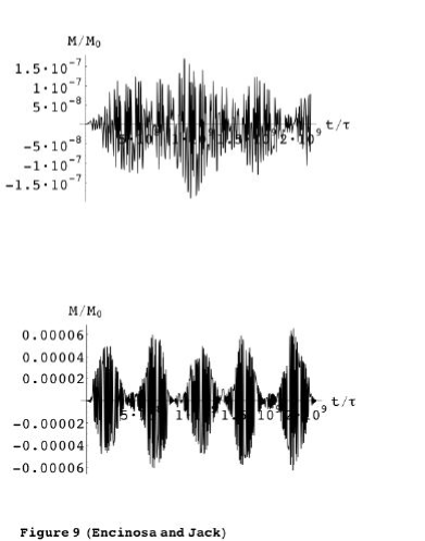
FIG 9. : Magnetic moments $M_{z}(t)$ (top) and $M_{\phi}(t)$ (lower) in units of $M_{0}=e\hbar R^{2}/4m$ at $\phi=\pi/2$ for the LPW case. The longest arrow is $.009J_{0}$.

FIG 10. : Magnetic moments $M_{z}(t)$ (top) and $M_{\phi}(t)$ (lower) in units of $M_{0}=e\hbar R^{2}/4m$ at $\phi=\pi/2$ for the CPW case.

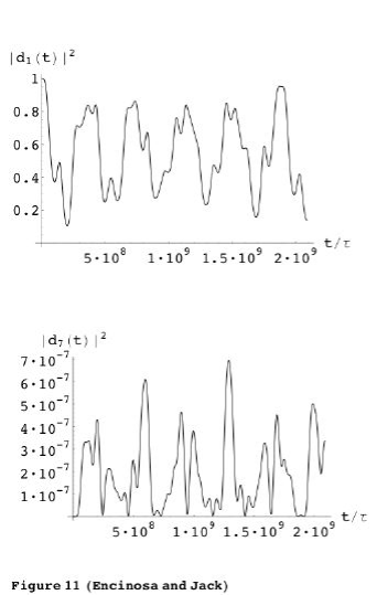
FIG 11. : Ground state $|d_{1}(t)|^{2}$ and seventh state $|d_{7}(t)|^{2}$ time dependent probability amplitudes for the system subjected to a LPW allowed to interfere with its reflection off an ideal mirror.

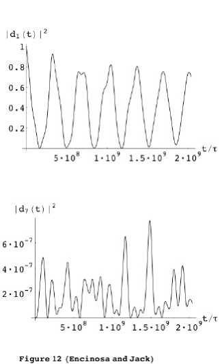
FIG 12. : Ground state $|d_{1}(t)|^{2}$ and seventh state $|d_{7}(t)|^{2}$ time dependent probability amplitudes for the system subjected to a CPW allowed to interfere with its reflection off an ideal mirror.

FIG 13. : $J^{b}_{\theta}(t_{f},\theta)$ plotted on the torus (in units of $R=1$) at $\phi=0$ in $\theta=\pi/4$ intervals for the CPW case where the wave is allowed to interfere with its reflection. A circulating SCD results. The longest arrow is $1.2\times 10^{-6}J_{0}$.

FIG 14. : $J^{b}_{\phi}(t_{f},\phi)$ plotted on the torus (in units of $R=1$) at $\theta=\pi$ in $\phi=\pi/4$ intervals for the CPW case where the wave is allowed to interfere with its reflection, showing that a circulating SCD results in the azimuthal direction as well as around the minor radius as per Fig. 13. The longest arrow is $1.5\times 10^{-2}J_{0}$.

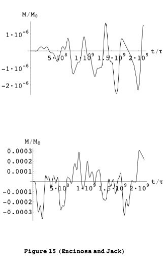
FIG 15. : Magnetic moments $M_{z}(t)$ (top) and $M_{\phi}(t)$ (lower) in units of $M_{0}=e\hbar R^{2}/4m$ at $\phi=\pi/2$ for the LPW case where the wave is allowed to interfere with its reflection.

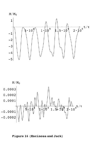
FIG 16. : Magnetic moments $M_{z}(t)$ (top) and $M_{\phi}(t)$ (lower) in units of $M_{0}=e\hbar R^{2}/4m$ at $\phi=\pi/2$ for the CPW case where the wave is allowed to interfere with its reflection.

References

• Shapiro and Brumer (2003) M. Shapiro and P. Brumer, Principles of the quantum control of molecular processes (John Wiley & Sons, Hoboken, NJ, 2003).
• Borzi et al. (2002) A. Borzi, G. Stadler, and U. Hohenester, Phys. Rev. A 66, 053811 (2002).
• Potz (1998) W. Potz, App. Phys. Lett. 72, 3002 (1998).
• Qin et al. (2003) H. Qin, D. W. van der Weide, J. Truitt, K. Eberl, and R. H. Blick, Nano. Lett. 14, 60 (2003).
• Oosterkamp et al. (1998) T. H. Oosterkamp, T. Fujisawa, W. G. van der Weil, K. Ishibashi, R. V. Hijman, S. Tarucha, and L. P. Kouwenhoven, Nature 395, 873 (1998).
• Bulaev et al. (2004) D. Bulaev, V. Geyler, and V. Margulis, Phys. B 69, 195313 (2004).
• Climente et al. (2005) J. I. Climente, J. Planelles, and F. Rajadell, J. Phys. Cond. Matt. 17, 1573 (2005).
• Tian and Datta (1994) W. Tian and S. Datta, Phys. Rev. B 49, 509 (1994).
• Filikhin et al. (2004) I. Filikhin, E. Deyneka, and B. Vlahovic, Modelling Simul. Mater. Sci. Eng. 12, 1121 (2004).
• Heinzel et al. (2001) T. Heinzel, K. Ensslin, W. Wegscheider, A. Fuhrer, S. L$\ddot{u}$scher, and M.Bichler., Nature 413, 822 (2001).
• Georgiev and Geller (2004) L. Georgiev and M. Geller, Phys. Rev. B 70, 155304 (2004).
• Gylfadottir et al. (2005) S. Gylfadottir, M. Nita, V. Gudmundsson, and A. Manolescu, Phys. E 27, 209 (2005).
• Ivanov and Lobanova (2003) A. Ivanov and O. Lobanova, Phys. E 23, 61 (2003).
• Latil et al. (2003) S. Latil, S. Roche, and A. Rubio, Phys. Rev. B 67, 165420 (2003).
• Pershin and Piermarocchi (2005a) Y. Pershin and C. Piermarocchi, Phys. Rev. B 72, 245331 (2005a).
• Pershin and Piermarocchi (2005b) Y. Pershin and C. Piermarocchi, Phys. Rev. B 72, 125348 (2005b).
• Sasaki et al. (2004) K. Sasaki, Y. Kawazoe, and R. Saito, Phys. Rev. A 321, 369 (2004).
• Sasaki and Kawazoe (2004) K. Sasaki and Y. Kawazoe, Prog. Theo. Phys. 112, 369 (2004).
• Simonin et al. (2004) J. Simonin, C. Proetto, Z. Barticevic, and G. Fuster, Phys. Rev. B 70, 205305 (2004).
• (20) S. Viefers, P. Koskinen, P. S. Deo, and M. Manninen, cond-mat /0310064.
• Encinosa and L.Mott (2003) M. Encinosa and L.Mott, Phys. Rev. A 68, 014102 (2003).
• Encinosa et al. (2005) M. Encinosa, L. Mott, and B. Etemadi, Phys. Scr. 72, 13 (2005).
• Encinosa (2006) M. Encinosa, Phys. Rev. A 73, 012102 (2006).
• Burgess and Jensen (1993) M. Burgess and B. Jensen, Phys. Rev. A 48, 1861 (1993).
• Jensen and Koppe (1971) H. Jensen and H. Koppe, Ann. of Phys. 63, 586 (1971).
• da Costa (1981) R. C. T. da Costa, Phys. Rev. A 23, 1982 (1981).
• da Costa (1982) R. C. T. da Costa, Phys. Rev. A 25, 2893 (1982).
• Matusani (1991) S. Matusani, J. Phys. Soc. Jap. 61, 55 (1991).
• Goldstone and Jaffe (1991) J. Goldstone and R. L. Jaffe, Phys. Rev. B 45, 14100 (1991).
• Exner and Seba (1989) P. Exner and P. Seba, J. Math. Phys. 30, 2574 (1989).
• Schuster and Jaffe (2003) P. C. Schuster and R. L. Jaffe, Ann. Phys. 307, 132 (2003).
• Kuhnel (1999) W. Kuhnel, Differential geometry (Friedr. Vieweg & Sohn Verlagsgesellschaft mbH, Wiesbaden, Germany, 1999).
• Garcia et al. (1997) J. M. Garcia, G. Medeiros-Ribeiro, K. Schmidt, T. Ngo, J. L. Feng, A. Lorke, J. Kotthaus, and P. M. Petroff, App. Phys. Lett. 71, 2014 (1997).
• Lorke et al. (2003) A. Lorke, S. Bohm, and W. Wegscheider, Superlattices Micro. 33, 347 (2003).
• Lorke et al. (2000) A. Lorke, R. J. Luyken, A. O. Govorov, and J. P. Kotthaus, Phys. Rev. Lett. 84, 2223 (2000).
• Zhang et al. (2003) H. Zhang, S. W. Chung, and C. A. Mirkin, Nano. Lett. 3, 43 (2003).
• Encinosa (a) M. Encinosa, physics /0501161.
• Encinosa (b) M. Encinosa, eprint unpublished.
Figures
Refer to caption