Chaotic Emission from Electromagnetic Systems Considering Self-Interaction

Abstract

The emission of electromagnetic waves from a system described by the Hénon-Heiles potential is studied in this work. The main aim being to analyze the behavior of the system when the damping term is included explicitly into the equations of motion. Energy losses at the chaotic regime and at the regular regime are compared. The results obtained here are similar to the case of gravitational waves emission, as long we consider only the energy loss. The main difference being that in the present work the energy emitted is explicitly calculated solving the equation of motion without further approximations. It is expected that the present analysis may be useful when studying the analogous problem of dissipation in gravitational systems.

I Introduction

I.1 Motivation

The chief motivation of the present work is trying to better understand the effects of damping forces (the radiation reaction forces) in radiating systems undergoing chaotic motions. Our ultimate interest is in gravitational systems, in particular, in the case of radiating chaotic systems. However, due to the difficulties that usually arise during the numerical evolution of equations from Einstein gravity, we start analyzing the electromagnetic analogous problem and shall use the experience acquired here to be able to circumvent those difficulties in future work dealing with gravitational systems.

In a classical field theory, the losses of energy and momenta due to the presence of radiation reaction forces is of fundamental importance to determine the physical properties of the system. Studies on this subject have been done in electromagnetic systems since Maxwell has established the foundations of the electromagnetic interaction, and in gravitational systems just after Einstein has formulated the theory of general relativity. Even though much progress have been done in both cases, there are still some points to be clarified.

Recent works about emission of gravitational waves from chaotic systems presented several interesting features of such systems. However, some important questions remained without answer. Particularly, the influence of the damping term to the dynamics of a chaotic system is not well understood. A major difficulty in studying the effects of radiation reaction in the dynamics of a (chaotic) gravitational system is the necessity of including higher order Post-Newtonian (PN) terms. Levin levin2000 has shown that at $2.0$ PN order, the two body problem with spin is chaotic, extending previous study of Suzuki and Maeda suzuki . Nevertheless, the effects of a dissipation term become important only with inclusion of $2.5$ PN order. So, in order to describe possible effects of chaotic emission on the detection of gravitational waves, it becomes important to consider higher order terms (see for example the comments from Cornish cornish and Hughes hughes ).

It has been shown that the amount of energy carried away by gravitational waves in a chaotic regime is smaller than in a regular regime kokubun (see also cornish ; suzuki ). However, this result was obtained by brute force method, because in Newtonian gravity, the emission of gravitational waves is dynamically unimportant, and in these works the energy emission was considered at Newtonian approximation. Thus, knowing the exact manner in which the emission of gravitational waves in a chaotic system is affected by the damping term is still an open question. The way to find the answer to this question is not as straightforward as we might naively think. In Einstein gravity, a damping term appears explicitly into the equations of motion for a test particle just after some type of approximation is performed. The exact form of the dissipation term depends not only on the coordinate system chosen, but depends also on the approximation technique used. This is a consequence of the non-linearity of the equations of motion. Moreover, the problem of gravitational radiation reaction usually involves enormously complicated calculations and are full of potential sources of errors which may lead to results whose physical meaning is difficult to be established.

On the other hand, the analogous problem of the electromagnetic radiation reaction is far easier to be analyzed and quite well understood. Much work on the subject has been done since the pioneering papers by Lorentz lorentz and Planck planck . The relativistic version of the radiation reaction force was derived by Abraham abraham and lately by Dirac dirac , and we can say that the effects of radiation reaction force on an accelerated particle, as a classical field theory in special relativity, is very well understood (see, e.g., jackson and references therein). The generalization of Dirac’s result to curved spacetimes was done by DeWitt and Brehme dewittbrehme , and by Hobbs hobbs . When considering the quantum theory, the classical electromagnetic radiation reaction force is also soundly based, since it can be obtained by taking the appropriate limit of a particular quantum electrodynamical process moniz . For instance, the position of a linearly accelerated charged particle in the Lorentz-Dirac theory is reproduced by the $\hbar\longrightarrow 0$ limit of the one-photon emission process in QED (See higuchi and Refs. therein). However, the study of chaotic radiating electromagnetic systems found in the literature refers mostly to quantum properties of such systems. Its classical counterpart was not investigated perhaps because the radiation reaction is really important in microscopic systems.

The similarity between the Abraham-Lorentz theory and the equations appearing in some approximation schemes from the general relativistic analogous problem of a radiating gravitational system (see e. g. Ref. pfenningpoisson ), and the simplicity of the electromagnetic case compared to the gravitational case, makes interesting to deepen the study on this subject. Therefore, we perform here the analysis of the effects of radiation reaction forces considering a classical electromagnetic chaotic system, and in a future work we investigate the gravitational case. We expect that the comparison of the results from the present work to future works considering gravitational systems, although different in characteristics, shed some light helping to better understand the gravitational radiation damping problem, particularly in chaotic systems (see e.g. kunze for the comparison among electromagnetic and gravitational non-chaotic damped systems).

I.2 The problem

In order to investigate the effects of radiation reaction on the dynamics of an electromagnetic chaotic system, we consider a charged test particle (it can be a macroscopic test particle) of mass $m$ and charge $q$ submitted to an external electrostatic field. In such a case, the non-relativistic motion of the test particle is governed by the equation ford1 ; rohrlich

$$m\frac{d\vec{v}}{dt}=\vec{F}_{\rm ext}+\tau_{\rm q}\frac{d\vec{F}_{\rm ext}}{dt},$$ (1)

where $\vec{F}_{\rm ext}$ denotes the external force acting on the charged particle, $\displaystyle{d\vec{F}_{\rm ext}\over dt}$ is the complete (convective) time derivative of the external force, and $\tau_{\rm q}=2q^{2}/(3mc^{3})$ is the characteristic dissipation time, which indicates how efficient is the energy emission. The last term of the above equation is the particle self-force which arises due to the emission of electromagnetic radiation, and is interpreted as a dissipative force. Accordingly, such a term is usually referred to as a damping term, and also as a dissipation term, both of which are used throughout this paper.

Accordingly, the names damping term, or dissipation term are also used.

The derivation of Eq. (1), and of its relativistic version, with some applications and with the interpretation of the dissipation term (and, in particular, of the parameter $\tau$) can be found in the classical textbooks landaulifshitz ; jackson . In fact, in the original derivation by Lorentz lorentz and Planck planck (the relativistic version was derived by Abraham abraham and Dirac dirac ) the resulting equation of motion is $m\,\vec{a}=\vec{F}_{\rm ext}+m\tau_{\rm q}\,(d\vec{a}/dt)$, which leads to runaway solutions. A way to avoid such a type of solutions is by replacing the time derivative of the particle’s acceleration $d\vec{a}/dt$ by the time derivative of the external force, $m(d\vec{a}/dt)={d\vec{F}_{\rm ext}/dt}$, into this equation, what yields Eq. (1) as a first approximation to the equation of motion for a charged particle. A deeper analysis, however, performed in Ref. rohrlich claims that Eq. (1) is the correct equation of motion for a charged particle submitted to an external force $\vec{F}_{\rm ext}$ (see also Refs. ford2 ; vogt ).

A further well known property of Eq. (1) is that, for motions within a time interval $\Delta t$ such that $\Delta t\ll\tau_{\rm q}$, the radiative effects on the dynamics of the system will be negligible, and the last term in Eq. (1) can be neglected. Thus, in order for the effects of the damping term to be noticeable, the time of observation must be large compared to $\tau_{\rm q}$. This is equivalent to say that the effects of dissipation will be important only for situations in which the external force is applied for a time interval $\Delta t$ much larger than the dissipation time $\tau_{q}$, $\Delta t\gg\tau_{q}$. These conditions were both taken into account in our simulations (see Sec. II.2). Hence, the system we are analyzing here can be interpreted as the analogous to the case of an orbiting test body in a weak gravitational field, but considering explicitly the damping term.

I.3 The structure of the paper

In the following section we write explicitly the equations of motion for a test charged particle in the Hénon-Heiles potential, by assuming a non relativistic motion. Sec. III is dedicated to report the numerical results and to their analysis. A brief analysis on the relativistic particle motion is done in Sec. IV, and finally in Sec. V we conclude by making a few remarks and final comments.

II Hénon-Heiles Systems

II.1 The model

We consider an external force $\vec{F}_{\rm ext}$ derived from a Hénon-Heiles electrostatic potential hh , and work in a non-relativistic regime where Eq. (1) holds (for a relativistic version of Eq. (1) see rohrlich ; ford2 ; see also Sec. IV). The choice of such a potential was due mainly to its simplicity allied to its dynamical richness, implying for instance chaotic motions, what is of capital importance in our analysis. Other interesting point to be mentioned is that a potential of the same type was used in a previous work which analyzed the emission of gravitational waves kokubun instead electromagnetic waves, and so the results of the two works can be compared. Hénon-Heiles systems are described by a potential of the form

$$V(x,y)=m\omega^{2}\frac{x^{2}+y^{2}}{2}+\frac{m\omega^{2}}{a}\left(x^{2}y-\frac{y^{3}}{3}\right),$$ (2)

and have been considered in several contexts vernov beyond the original astrophysical scenario. This potential is basically a perturbed two-dimensional harmonic oscillator. Therefore, $\omega$ may be identified with the oscillatory frequency which, in the absence of the perturbation term, is $\omega=\sqrt{k/m}$, $k$ being a spring constant, for a mechanical system or $\omega=\sqrt{|Qq|/ma^{3}}$, where $Q$ and $q$ are respectively the source and the test particle charges, for an electric system (in CGS-Gaussian units). Parameter $a$ is the characteristic length of the system. The characteristic frequency $\omega$ defines a characteristic period of motion, $T=\omega^{-1}$.

Without the damping term, and with the usual choice of units hh , $m=\omega=a=1$, and in our case also $Q=q=1$ (see below), the chaoticity of the Hénon-Heiles system is controlled only by its energy $E$: the system is bound if $E\lesssim 1/6$, being mostly regular for the energy range from $0$ to nearly $1/10$, and being mostly chaotic for $E$ in the range $1/10$ to $1/6$.

In the presence of the damping term, the dynamics of a charged point particle in the potential given by equation (2) is governed by the equations

$$\ddot{x}+\omega^{2}x = -2\frac{\omega^{2}}{a}xy-\tau_{q}\omega^{2}\left[\dot{x}+2\frac{1}{a}\left(x\dot{y}+y\dot{x}\right)\right]\,,$$ (3)

$$\ddot{y}+\omega^{2}y = -\frac{\omega^{2}}{a}\left(x^{2}-y^{2}\right)-\tau_{q}\omega^{2}\left[\dot{y}+2\frac{1}{a}\left(x\dot{x}-y\dot{y}\right)\right]\,.$$ (4)

Here, working with electromagnetic field and using Eqs. (3) and (4), we considered the effects of radiation damping, comparing long term energy loss between chaotic and regular regimes. The energy loss being considered directly into the equations of motion without further approximations. The main results are reported and analyzed in Sec. III.

II.2 Units and normalized parameters

We present here a discussion about the physical parameters of the present Hénon-Heiles electromagnetic system. However, let us stress once more that the present model is to be considered a toy model, as a laboratory test for our procedures, and not as a test for the electromagnetic theory.

Eqs. (3) and (4) have three free parameters characteristic to the system under consideration: The constant $a$, the characteristic time $\tau_{\rm q}$, and the frequency $\omega$. Then we follow the standard procedure and choose a new normalized time parameter $\tau$ and a new normalized time variable $t$ given respectively by the relations $\tau=\tau_{\rm q}\times\omega$, and $t=t(s)\times\omega$, where $\tau_{\rm q}$ and $t(s)$ carry dimensions, while $\tau$ and $t$ are dimensionless parameters. The constant $a$, which carries dimensions of length, is used to normalize the variables $x$ and $y$. The usual choice is to measure $x$ and $y$ in units of $a$, which is equivalent to making $a=1$ into the equations of motion.

As far as the effects of dissipation are concerned, the important parameter is the rationalized characteristic time $\tau$. The contribution of the radiation reaction force to the dynamics of the system is proportional to $\tau$ (see Eq. 1). Therefore, the value to be chosen for $\tau$ has to be as large as possible. On the other hand, as shown below, the time of observation (the computation time) has to be much larger than $\tau$ in order for the effects of dissipation being noticeable.

Considering the motion of charged elementary particles, the largest value for $\tau_{\rm q}$ follows when the test particle is an electron, in which case one has $\tau_{\rm q}\equiv\tau_{\rm e}\simeq 6.3\times 10^{-24}s$. If the test particle is a proton then $\tau_{q}\simeq 3.4\times 10^{-27}s$. For macroscopic systems, however, the ratio $q/m$ is not fixed and $\tau_{q}$ may assume values several orders of magnitude larger than $\tau_{\rm e}$. For a charged test body such that $q=\alpha e$ and $m=\beta m_{\rm e}$ one has $\tau_{\rm q}=(\alpha^{2}/\beta)\tau_{\rm e}$. Take, for instance, a test body of mass $m=10g$ and charge $q=1.0\times 10^{7}\,\rm{esu}\simeq 3.3\times 10^{-3}C$. Then, it follows $\alpha=2.1\times 10^{16}$, $\beta=1.1\times 10^{28}$, and $\tau_{\rm q}=2.5\times 10^{-19}s$.

Regarding to the third parameter of the model, the characteristic frequency $\omega$, one sees that it depends also upon the source of the Hénon-Heiles potential, being a typical period of the system. For an electromagnetic system it is related to the total charge $Q$ of the source by a relation of the form, $m\omega^{2}=Qq/a^{3}$, $m$ and $q$ being respectively the mass and the electric charge of the test particle, and $a$ being the characteristic length of the system mentioned above. As usual in Hénon-Heiles systems, we are free to fix $\omega$ as an inverse time unit, $\omega=\omega_{q}$, in such a way that $\tau=\tau_{q}\omega_{q}$. Thus, if the source of the potential has mass $m=\beta m_{e}$ and net electric charge $q=\alpha e$, we have

$$\tau=\tau_{q}\omega_{q}=\frac{\alpha^{2}}{\beta}\tau_{e}\omega_{q}\,.$$ (5)

Therefore, if we think of a specific orbiting particle ($\tau_{q}$ fixed), different values of the dissipation parameter mean different values for $\omega_{q}$, which gives the corresponding physical parameters of the Hénon-Heiles potential.

Now we are ready to fix the parameters and to establish some constraints to the physical size of our system. Let us consider a system with typical size $L$ (which is essentially of the order of the parameter $a$ mentioned above). Being $\omega_{q}^{-1}$ a typical period, we have that $L\omega_{q}$ is a typical velocity of the system. Such a velocity has to be smaller than the speed of light $c$, i.e., $L\omega_{q}\leq c$, so that we have the following upper bound for the system size

$$L\lesssim c\omega_{q}^{-1}=c\frac{\tau_{e}}{\tau}\frac{\alpha^{2}}{\beta}\simeq 2\times 10^{-13}\frac{\alpha^{2}}{\tau\beta}\;\rm{cm}.$$ (6)

As we shall see below, physically interesting values of $\tau$ for which the numerical results can be clearly interpreted lay in the interval $\tau\in[10^{-10},10^{-4}]$. Considering such a range for $\tau$ and taking an electron as the test particle, for which $\alpha=\beta=1$, we obtain the typical size of the system as $L\lesssim 2\times 10^{-9}\rm{cm}$ for $\tau=10^{-4}$, and $L\lesssim 2\times 10^{-3}\rm{cm}$ for $\tau=10^{-10}$. On the other hand, if the test body has mass $m=10g$ and charge $q=10^{7}\rm{esu}$ ($\alpha=2.1\times 10^{16}$, $\beta=1.1\times 10^{28}$), we obtain respectively, $L\lesssim 8\times 10^{-5}\,\rm{cm}$ and $L\lesssim 80\rm{cm}$. If the test particle is an electron, the typical size of the system is microscopic which is more difficult to be managed. Thus, in order to consider a possible experimental setup, it will be certainly more feasible to work with a macroscopic test particle. However, the choice of $\tau$ in the above range describes both the microscopic and the macroscopic systems.

One more issue on the subject of fixing parameters concerns the physical properties of the source in the Hénon-Heiles system. Namely, the electric charge $Q$ and the characteristic length $a$. As we have seen above, these are related to the characteristic frequency $\omega_{q}$, and once we have normalized units through Eqs. (5) and (6), the ratio $Q/a^{3}$ is fixed as soon as we fix the dissipation parameter $\tau$. From the above definitions and choices it is found $Q\sim 1.7\times 10^{3}\beta\,L/\alpha\,\,(\rm{CGS})$, where we assumed that the characteristic size of the source is of the same order of magnitude as the parameter $L$ defined in Eq. (6). Hence, in the case of the preceding examples it gives the upper limits $Q\sim 3.6\,\rm{esu}$ and $3.6\times 10^{-6}\,\rm{esu}$ for the microscopic orbiting particle, respectively with $\tau=10^{-10}$ and $\tau=10^{-4}$. And for the macroscopic orbiting particle we find $Q\sim 7.1\times 10^{16}\,\rm{esu}$ and $7.1\times 10^{10}\,\rm{esu}$, respectively, for $\tau=10^{-10}$ and $\tau=10^{-4}$.

III Numerical simulations and results

III.1 Methodology

Equations (3) and (4) were solved numerically. For the sake of comparison, we initially used two different numerical methods: a fourth order Runge-Kutta with fixed stepsize and a Runge-Kutta with adaptive stepsize NR . Also, we used MATHEMATICA built-in procedures for solving Ordinary Differential Equations.

At first, we integrated Eqs. (3) and (4) considering no dissipation term, i.e., with $\tau=0$. The initial conditions were generated at random, fixing only initial energy and choosing $x=0$ at the start. Since in this case the system is conservative, the energy is a constant of motion, and its value was used to check and compare the numerical results obtained through different methods. No significant differences were observed, so we adopted a fourth order Runge-Kutta in our simulations.

III.2 Numerical simulations

The main concern of this work is answering the question: How does the value of the dissipation time $\tau$ affect the dynamics of system? In particular, we also want to know how much energy is radiated by the accelerated particle undergoing chaotic motions in comparison to regular motions. It is expected that a large value of $\tau$ will strongly affect the dynamics, in opposition to small values, for which the dynamics of the system should be weakly affected. Nonetheless, it remains to be defined what values of $\tau$ can be considered large and what are small ones. For comparison we made simulations for several different values of $\tau$ and same initial conditions. After a few tries, we have chosen five particular cases to analyze in more detail. The chosen values are $\tau=0,\;10^{-4},\;10^{-6},\;10^{-8}$, and $10^{-10}$, with initial energy $E=0.12$ and the same initial conditions for all of the five cases.

The results can be seen in Fig. 1, where we plot the Poincaré sections for each value of $\tau$. Each one of the graphs represents the resulting section for only one orbit, corresponding to the particular initial conditions we have chosen. Notice that except for $\tau=10^{-4}$, all other Poincaré sections look very similar, suggesting that $\tau\sim 10^{-4}$ or greater are to be considered large values, and $\tau$ is to considered small if its value is of the order of $10^{-6}$ or below.

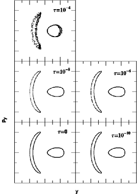
Figure 1: Poincaré sections for $E=0.12$ and several values of $\tau$. All sections with the same initial conditions.

In order to better understand the behavior of the Poincaré sections we evaluate the percent amount of radiated energy $\Delta E$ as a function of time in each case shown in Fig. 1 The results are seen in Fig. 2 where we plot the graphics of $\Delta E\times t$ for each case. Note that these graphs are the actual data points, and not fits adjusting the data. For instance, the lines appearing in the first four graphs of that figure are the result of plotting the set of points obtained numerically for each one of the particular orbits chosen to be analyzed. Such straight lines indicate that energy emission rate is constant, and that the total energy of the system decreases linearly with time. This is so for small dissipation times $\tau$, while for higher values of $\tau$ the energy loss rate is not constant with time (see Fig. 3). It is seen that for $\tau=0$ the variations in the energy are exceedingly small ($\sim 10^{-11}\,\%$) and look like random variations. This is surely not an effect of dissipation, because the total energy dissipated during the integration time is essentially zero. These random variations are caused by numerical inaccuracy, as it can be inferred by comparing this to the other cases with $\tau\neq 0$, where the energy variations are much larger and systematic, causing the energy to decrease monotonically with time. For instance, for $\tau=10^{-4}$ the total energy dissipated during the integration time reaches nearly $20\,\%$ of the initial value, so that at time $t\simeq 2000$ the energy of the system is about $E\simeq 0.096$. On the other hand, for $\tau=10^{-6}$ the energy variation reaches nearly $0.20\%$ of its initial value in the same integration time, and the energy is reduced to nearly $E\simeq 0.1197$, meaning it is almost a constant of motion. Also for $\tau=10^{-8}$ and $10^{-10}$ the energy variations reach $\sim 10^{-3}\,\%$ and $\sim 10^{-5}\,\%$, respectively. Even though these energy variations are quite small, they are about eight (for $\tau=10^{-8}$) and six (for $\tau=10^{-10}$) orders of magnitude larger then in the case $\tau=0$, and yet we can see they cause the energy of the system to decrease monotonically with time.

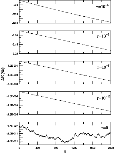
Figure 2: Percentage of energy loss for five values of $\tau$, as indicated in the figure. Initial energy is E=0.12, and the same initial conditions were used for all cases, as in Fig. 1.

As a further example of a large (higher) $\tau$ value, we performed simulations with $\tau=10^{-3}$ and with energy $E=0.12$, and the results are seen in Fig. 3. The large graphics shows the percent variations of the energy, and the small graph is the Poincaré section for this special orbit. Due to the large dissipation parameter, the motion is highly damped and, after some time, rest is attained. At time $t=2000$ nearly $90\%$ of the initial energy has been carried away by electromagnetic radiation. Note also that the amount of energy emitted does not vary linearly with time, as it happens for smaller values of $\tau$.

For our purposes here, high values of $\tau$, $\tau\gtrsim 10^{-4}$, say, are not interesting because the dynamics of the system is highly affected and the comparison to the case without dissipation becomes difficult (if not impossible) to be done. Then, we considered only $\tau=10^{-6},\;\tau=10^{-8}$, and $\tau=10^{-10}$ in our full simulations.

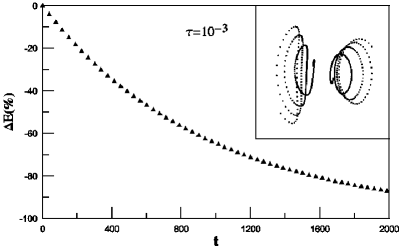
Figure 3: Energy emission with high $\tau$ term as a function of time. The small graphics is the Poincaré section of the motion. The initial energy is $E=0.12$ and $\tau=10^{-3}$.

Once fixed the values of $\tau$, the next step was solving numerically Eqs. (3) and (4) with several initial conditions, and for the energy values $E=0.12$ and $E=0.14$. A set of $500$ distinct initial conditions was generated using a (pseudo) random number generator RN , and the same set was used for every combination of the controlled parameters, $\tau\in\{0,\;10^{-6},\;10^{-8},\;10^{-10}\}$ and $E\in\{0.12,\;0.14\}$. For each pair of these parameters we performed $500$ simulation, with the $\tau=0$ case being included only for comparison purposes.

Although we performed simulations also for $E=0.09$ and $E=0.10$, the respective results were not considered in our analysis. In such cases, the number of chaotic motions (typically less than $10$ in $500$ simulations) in our set of results was too small for a good statistics, and so they would not be useful in comparing chaotic to regular regimes, which is the basic aim of the present work.

III.3 Results and analysis

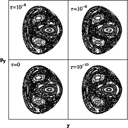
Figure 4: Poincaré sections for $E=0.12$ and four values of $\tau$, as indicated in each graphics, corresponding to $500$ distinct initial conditions in each plot.

Using the results of our simulations, we constructed Poincaré section for each case, all of them being drawn on the surface $x=0$ in phase space. These sections were analyzed in order to separate between dynamics with chaotic motions from dynamics with regular motions.

The graphics in Fig. 4 are Poincaré sections obtained for $E=0.12$, without damping term ($\tau=0$), and with dissipation term for $\tau=10^{-10}$, $\tau=10^{-8}$, and $\tau=10^{-6}$, as indicated in each plot. Although the overall aspects are the same, a detailed analysis of individual sections reveals different aspects as seen in Fig. 5, where we plot Poincaré sections for particular orbits corresponding to three different sets of initial conditions for each value of $\tau$. Here a very important result is that with the inclusion of a small damping term, the overall aspect of motions are the same, and in particular, the energy is nearly constant, so that Poincaré section is still a good tool in order to classify the motions as regular or chaotic. From this figure it is also seen the dependence of the dynamics on the initial conditions, besides the dependence upon $\tau$. It is also worth saying that a few particular orbits, out of the 500 initially chosen, were neglected since it was not clear from the obtained Poincaré sections whether they correspond to regular or chaotic motions (see Table 1).

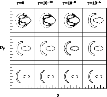
Figure 5: Poincaré sections for $E=0.12$ and four distinct values of $\tau$, but with the same initial conditions, are shown at the same horizontal level. The corresponding $\tau$ values appear on top of each column.

Now with our set of simulations already separated into two sets, one set with ordered motions only and the other set with chaotic ones, we calculated for each initial condition (in each set) a best linear fit to the energy variations $\Delta E=At+B$, determining $A$ and $B$ by using standard techniques of linear regression. Then, with such a set of values for $A$ and $B$ we determined the mean values $<A>$ and $<B>$, and their respective standard deviations, $\sigma_{A}$ and $\sigma_{B}$, for each regime of motions. The results are summarized in Table 1, where we show just the values of $<A>$ and $\sigma_{A}$. These are more important than the values of $<B>$ and $\sigma_{B}$, because they furnish the (time) rate of energy carried away by electromagnetic waves. We also show in that table (last column), the resulting number of regular and chaotic motions for each pair of values of the initial energy and dissipation time. As mentioned above, some orbits are missing because they could not be classified as regular nor as chaotic ones.

$E=0.12$

$\tau$ $\qquad<A>$ $\qquad\sigma_{A}$ Regime $\;\#$ $10^{-6}$ $-9.92\times 10^{-5}$ $-9.24\times 10^{-5}$ $1.33\times 10^{-5}\;$ $3.99\times 10^{-6}$ Regular Chaotic 282 202 $10^{-8}$ $-1.02\times 10^{-6}$ $-9.18\times 10^{-7}$ $1.29\times 10^{-7}\;$ $5.39\times 10^{-8}$ Regular Chaotic 236 260 $10^{-10}$ $-1.08\times 10^{-8}$ $-9.09\times 10^{-9}$ $9.09\times 10^{-10}$ $6.90\times 10^{-10}$ Regular Chaotic 163 337

$E=0.14$

$10^{-6}$ $-1.05\times 10^{-4}$ $-9.06\times 10^{-5}$ $1.53\times 10^{-5}\;$ $4.76\times 10^{-6}$ Regular Chaotic 146 350 $10^{-8}$ $-1.06\times 10^{-6}$ $-9.05\times 10^{-7}$ $1.51\times 10^{-7}\;$ $5.28\times 10^{-8}$ Regular Chaotic 141 359 $10^{-10}$ $-1.12\times 10^{-8}$ $-9.06\times 10^{-9}$ $7.97\times 10^{-10}$ $7.42\times 10^{-10}$ Regular Chaotic $\;96$ 403

Table 1: Mean values of the energy loss rates $<A>$, and the standard deviations $\sigma_{A}$ for each energy and $\tau$ values. The last column shows the number of motions in each particular regime.

With the obtained data, we compared the amount of energy radiated in regular regimes with respect to chaotic regimes, and calculated the percent ratio $\eta$ as follows

$$\eta=\frac{<A>_{R}-<A>_{C}}{<A>_{C}}\times 100,$$ (7)

where the subscript $C$ stands for chaotic and subscript $R$, for regular. This is shown in Table 2. In all cases the average energy radiated in regular regimes is larger than in chaotic regimes. These results are compatible with what was obtained when considering gravitational waves emission kokubun ; suzuki (see also levin2000 ; cornish ).

$E$	$\tau$	$\eta$ (%)
$0.12$	$10^{-6}$	7%
0.12	$10^{-8}$	11%
0.12	$10^{-10}$	18%
0.14	$10^{-6}$	16%
0.14	$10^{-8}$	17%
0.14	$10^{-10}$	24%

Table 2: The percent values of energy emitted by the system in a regular regime with respect to a chaotic regime.

IV Relativistic motion

We have also investigated the behavior of the electromagnetic Hénon-Heiles system in relativistic dynamics. In such a case we solved the equations rohrlich ; jackson

$${d\vec{p}\over dt}=\vec{F}+\tau\gamma{d\vec{F}\over dt}-\tau{\gamma^{3}\over c^{2}}{d\vec{v}\over dt}\times\left(\vec{v}\times\vec{F}\right)\,,$$ (8)

where $\vec{p}=\gamma m\vec{v}$, $\gamma=1/\sqrt{1-v^{2}\,}$, and $\vec{F}$ is the external force given by $\vec{F}=-\vec{\nabla}U$, U being the potential function given by Eq. (2). The explicit form of Eqs. (8), analogous to Eqs. (3) and (4), were used in the numerical calculations.

The numerical results obtained from the relativistic equation (8) were essentially the same as in the non-relativistic case. This can be understood noticing that for the bound system the particle undergoes a non-relativistic motion, as can be verified by the following facts. In the Hénon-Heiles potential (2), for the test particle to acquire velocities comparable to the velocity of light, its initial energy $E$ has to be large. In the rationalized units used here, this means $E\sim 1$. However, as shown in Ref. hh , if $E$ is larger than $1/6$ the system is not bound, and then in the regime where relativistic effects become important the particle is not bound by the Hénon-Heiles potential. Therefore, the relativistic regime is not important in the present analysis.

V Final remarks

Our results show that when we consider explicitly the effects of radiation reaction force, the energy emission through electromagnetic waves in the chaotic regime is smaller than in the regular regime, as it was in the case of emission of gravitational waves.

The ratio of energy loss in regular compared to chaotic motions increases with the initial energy of the system, and decreases with the dissipation parameter. Since in Hénon-Heiles systems the chaoticity increases with the energy, this means that the ratio between the energy emitted in regular motions and in chaotic motions grows with the chaoticity of the system.

We recall that, in the gravitational waves case, the simulations were performed at PN approximation lower than 2.5PN. The result was that the effect of gravitational waves emission is negligible to the dynamics of the system. However, being PN lower than $2.5$, in those simulations the effects of radiation emission were in fact not fully considered. In our analysis of the electromagnetic Hénon-Heiles system, these effects are fully considered through the radiation reaction force. Another important result is related to the mean life-time of source. If we make a prediction considering only regular dynamics its mean life-time may be shorter than the prediction from chaotic dynamics. However, in the case of dissipation by emission of gravitational radiation a more careful analysis has to be done.

The numerical procedures and analysis performed in this work will certainly be useful in our task of studying the gravitational analogous problem, the one about the gravitational radiation emitted by a particle undergoing chaotic motion, considering explicitly the damping term into the equations of motion (work on this subject is in progress).

References

- (1) J. Levin, Phys. Rev. Lett. 84, 3515 (2000).
- (2) S. Suzuki and K. I. Maeda, Phys. Rev. D 55, 4848 (1997).
- (3) N. J. Cornish, Phys. Rev. Lett. 85, 3980 (2000).
- (4) S. A. Hughes, Phys. Rev. Lett. 85, 5480 (2000).
- (5) F. Kokubun, Phys. Rev. D 57, 2610 (1998).
- (6) A. H. Lorentz, Arch. Neérl. 25, 363 (1892), see also A. H. Lorentz, Theory of Electrons (Dover, New York, 1952).
- (7) M. Planck, Ann. d. Phys. 296, 577 (1897).
- (8) M. Abraham, Ann. d. Phys. 319, 236 (1904).
- (9) P. A. M. Dirac, Proc. Roy. Soc. (London) A 167, 148 (1938).
- (10) J. D. Jackson, Classical Electrodynamics (John Wiley and Sons, New York, 1975).
- (11) B. S. DeWitt and R. W. Brehme, Ann. Phys. (NY) 9, 220 (1960).
- (12) J. M. Hobbs, Ann. Phys. (NY) 47, 141 (1968).
- (13) E. J. Moniz and D. H. Sharp, Phys. Rev. D 10, 1133 (1974).
- (14) A. Higuchi and G. D. R. Martin, Phys. Rev. D 70, 081701(R) (2004).
- (15) M. J. Pfenning and E. Poisson, Phys. Rev. D 65, 084001 (2002).
- (16) M. Kunze and A. D. Rendall, Classical Quantum Gravity 18, 3573 (2001).
- (17) G. W. Ford and R. F. O’Connell, Phys. Lett. A 157, 217 (1991).
- (18) F. Rohrlich, Phys. Lett. A 283, 276 (2001).
- (19) L. D. Landau and E. M. Lifshitz, Teoriya Polya (Nauka, Moscow, 1941), later French translation: Théorie du Champ (MIR, Moscow, 1966).
- (20) G. W. Ford and R. F. O’Connell, Phys. Lett. A 174, 182 (1993).
- (21) D. Vogt and P. S. Letelier, Gen. Relativ. Gravit. 35, 2261 (2003).
- (22) M. Hénon and C. Heiles, Astron. J. 69, 73 (1964).
- (23) S. Y. Vernov, Theor. Math. Phys. 135, 792 (2003).
- (24) W.H. Press, S.A. Teukolsky, W.T. Vetterling and B.P. Flannery, Numerical Recipes in FORTRAN, Cambridge Press (1992).
- (25) G. Marsaglia, A. Zaman, Toward a Universal Random Number Generator, Florida State University Report: FSU-SCRI-87-50 (1987), see also G. Marsaglia, A. Zaman and W.W. Tsang, Statistics Prob. Lett.9, 35 (1990) and G. Marsaglia, A. Zaman and W.W.Tsang, Comp. Phys. Commun.,60, 345 (1990).