Epidemic spreading in lattice-embedded scale-free networks

Abstract

We study geographical effects on the spread of diseases in lattice-embedded scale-free networks. The geographical structure is represented by the connecting probability of two nodes that is related to the Euclidean distance between them in the lattice. By studying the standard Susceptible-Infected model, we found that the geographical structure has great influences on the temporal behavior of epidemic outbreaks and the propagation in the underlying network: the more geographically constrained the network is, the more smoothly the epidemic spreads, which is different from the clearly hierarchical dynamics that the infection pervades the networks in a progressive cascade across smaller-degree classes in Barabási-Albert scale-free networks.

, ,

1 Introduction

The classical mathematical approach to disease spreading either ignores the population structure or treats populations as distributed in a regular medium [1]. However, it has been suggested recently that many social, biological, and communication systems possess two universal characters, the small-world effect [2] and the scale-free property [3], which can be described by complex networks whose nodes represent individuals and links represent the interactions among them [4]. In view of the wide occurrence of complex networks in nature, it is important to study the effects of topological structures on the dynamics of epidemic spreading. Pioneering works [5, 6, 7, 8] have given some valuable insights of that: for small-world networks, there are critical thresholds below which infectious diseases will eventually die out; on the contrary, even infections with low spreading rates will prevail over the entire population in scale-free networks, which radically changes many of the conclusions drawn in classic epidemic modelling. Furthermore, it was observed that the heterogeneity of a population network in which the epidemic spreads may have noticeable effects on the evolution of the epidemic as well as the corresponding immunization strategies [8, 9, 10].

In many real systems, however, individuals are often embedded in a Euclidean geographical space and the interactions among them usually depend on their spatial distances [11]. Also, it has been proved that the characteristic distance plays a crucial role in the phenomena taking place in the system [12, 13, 14, 15]. Thus, it is natural to study complex networks with geographical properties. Rozenfeld et al. considered that the spatial distance can affect the connection between nodes and proposed a lattice-embedded scale-free network (LESFN) model [12] to account for geographical effects. Based on a natural principle of minimizing the total length of links in the system, the scale-free networks can be embedded in a Euclidean space without additional external exponents. Since distributions of individuals in social networks are always dependent on their spatial locations, the influence of geographical structures on epidemic spreading is of high importance, but up to now it has rarely been studied except for [16, 17].

In this paper, we study the standard Susceptible-Infected (SI) model on the LESFNs, trying to understand how the geographical structure affects the dynamical process of epidemic spreading. Especially, we consider the temporal behavior of epidemic outbreaks and the propagation in the underlying network. It is found that the geographical structure plays an important role in the epidemic outbreaks and the propagation of diseases.

2 The model

According to Ref. [12], the LESFN is generated as follows: (i) a lattice of size $N=L\times L$ with periodic boundary conditions is assumed, upon which the network will be embedded; (ii) for each site, a preset degree $k$ is assigned taken from the scale-free distribution, $P(k)\sim k^{-\gamma}$, $m<k<K$; (iii) a node (say $i$, with degree $k_{i}$) is picked out randomly and connected to its closest neighbors until its degree quota $k_{i}$ is realized or until all sites up to a distance, $r(k_{i})=A\sqrt{k_{i}}$, have been explored. Duplicate connections are avoided. Here, $r(k_{i})$ is the spatial distance on a Euclidean plane, denoting the characteristic radius of the region that node $i$ can almost freely connect to the others; (iv) this process is repeated throughout all the sites on the lattice. Following this method, networks with $\gamma>2$ can be successfully embedded up to a (Euclidean) distance $r(k)$, which can be made as large as desired depending upon the change of the territory parameter $A$. Especially, the model turns out to be a randomly connected scale-free network when $A\rightarrow\infty$ [18]. Typical networks with $\gamma=2.5$ resulting from the embedding method are illustrated in Fig. 1. The power-low degree distributions of the LESFNs achieve their natural cutoff lengths for $A=2$, $3$, and $9$, respectively. While for $A=1$, the network ends at some finite-size cutoff length.

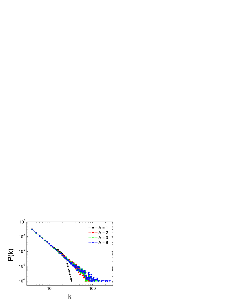
Figure 1: (Color online) Degree distribution of an LESFN model with $N=10000$, $\gamma=2.5$, and for different values of $A$. The territory parameter $A$ controls the influence of the geographical distance on the network structure.

In order to study the dynamical evolution of epidemic outbreaks, we focus on the standard SI model [1]. In this model, individuals have only two discrete states: susceptible (or healthy) and infected. Each individual is represented by a vertex of the network and the links are the connections between individuals along which the infection may spread. There are initially a number of $I_{0}$ infected nodes and any infected node can pass the disease to its susceptible neighbors at a spreading rate $\lambda$. Once a susceptible node is infected, it remains in this state. The total population (the size of the network) $N$ is assumed to be constant and, if $S(t)$ and $I(t)$ are the numbers of susceptible and infected individuals at time $t$, respectively, then $N=S(t)+I(t)$. In spite of its simplicity, the SI model is a good approximation for studying the early dynamics of epidemic outbreaks [1, 10] and assessing the effects of the underlying topologies on the spreading dynamics [15, 19].

3 Simulation results

We have performed Monte-Carlo (MC) simulations of the SI model with synchronously updating on the LESFNs. With relevance to empirical evidence that many networks are characterized by a power-low distribution with $2<\gamma<3$ [4], we set $\gamma=2.5$ in the present work. Initially, we select one node randomly and assume it is infected. The disease will spread throughout the network and the dynamical process is controlled by the topology of the underlying network.

Figure 2: (Color online) Density of infected individuals versus MC time in the LESFNs for different values of $\lambda$ and $A$. (a) $A=9$, $\lambda=0.001$ (solid line), $0.002$ (dash line), $0.003$ (dot line), and $0.005$ (dash-dot line), respectively. (b) $\lambda=0.001$, $A=1$ (solid line), $2$ (dash line), $3$ (dot line), and $4$ (dash-dot line), respectively. The network size is $N=10000$. All the plots were averaged over $500$ experiments.

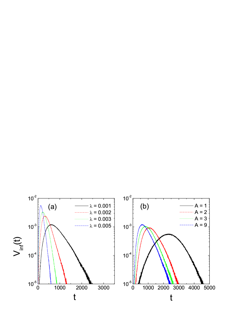
Figure 3: (Color online) Linear-log plots of spreading velocity in the LESFNs for different values of $\lambda$ and $A$. The network size is $N=10000$. All the curves were averaged over $500$ realizations. The symbols are the same as in Fig. 2.

In Fig. 2, we report the temporal behavior of outbreaks in the LESFNs. The density of infected individuals, $\rho(t)$ ($=I(t)/N$), is computed over $500$ realizations of the dynamics. Consistent with the definition of the model, all the individuals will be infected in the long-time limit, i.e., $\lim_{t\rightarrow\infty}\rho(t)=1$, since infected individuals remain unchanged during the evolution. In Fig. 2(a), for the given connecting region ($A=9$), the greater the spreading rate $\lambda$ is, the more quickly the infection spreads. Fig. 2(b) shows the dependence of the infectious prevalence $\rho(t)$ on the territory parameter $A$, while the spreading rate is fixed at $\lambda=0.001$. As $A$ increases from $1$ to $9$, the average spatial length of edges increases [12]; namely, the nodes have larger probabilities to connect to more other nodes, which therefore leads to a faster spread of the infection.

To better understand the virus propagation in the population, we study in detail the spreading velocity, written as [20]

$$V_{inf}(t)=\frac{d\rho(t)}{dt}\approx\rho(t)-\rho(t-1).$$ (1)

We count the number of newly infected nodes at each time step and report the spreading velocity in Fig. 3. Apparently, the spreading velocity goes up to a peak quickly and leaves very short response time for us to develop control measures. Before the outbreaks of the infection, the number of infected individuals is very small, lasting for a very long time during the outbreak, and the number of susceptible individuals is very small. Thus, when $t$ is very small (or very large), the spreading velocity is close to zero. In the case of $A=9$ (Fig. 3(a)), all plots show an exponential decay in the long-time propagation. These results are weakened for a small circular connecting probability (in particular, for $A=1$), as shown in Fig. 3(b), where the disease spreads in a relatively low velocity, which therefore slows down the outbreaks.

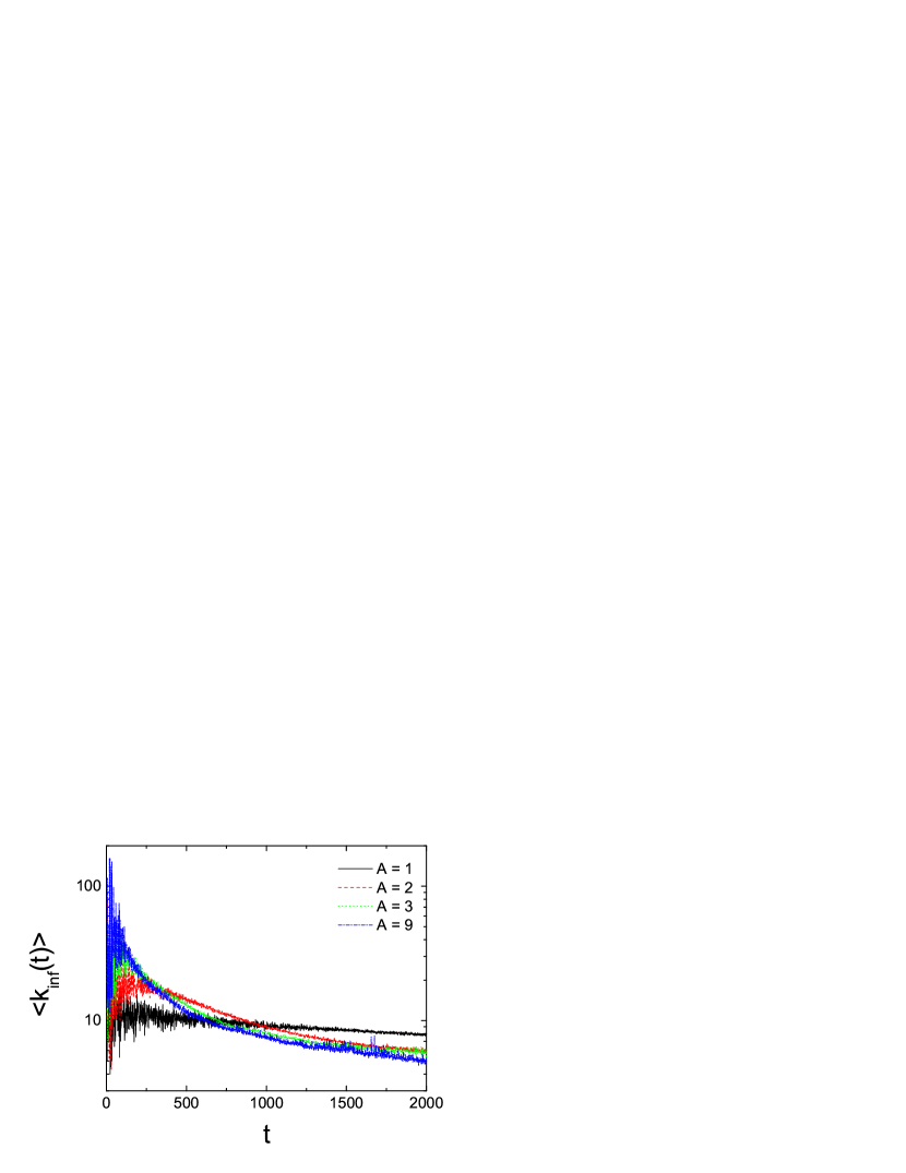
Figure 4: (Color online) Temporal behavior of the average degree of the newly infected nodes for the SI model outbreaks in the LESFNs with $N=10000$ and $\lambda=0.001$. The data are averaged over $500$ dynamical processes.

A more precise characterization of the epidemic diffusion through such a network can be achieved by studying the average degree of the newly infected individuals at time $t$ [10], given by

$$\langle k_{inf}(t)\rangle=\frac{\sum_{k}kI_{k}(t)-\sum_{k}kI_{k}(t-1)}{I(t)-I(t-1)},$$ (2)

where $I_{k}(t)$ is the number of infected nodes with degree $k$. In Fig. 4, we plot the temporal behavior of $k_{inf}(t)$ for the SI model with $\lambda=0.001$ in the LESFNs. Different from the clearly hierarchical dynamics in Barabási-Albert scale-free networks [10], in which the infection pervades the networks in a progressive cascade across smaller-degree classes, epidemic spreads slowly from higher- to lower-degree classes in the LESFNs. The smaller the territory parameter $A$ is, the more smoothly the infection propagates. Especially, strong global oscillations arise in the initial time region, which implies that the geographical structure plays an important role in early epidemic spreading, independent of the degrees of the infected nodes.

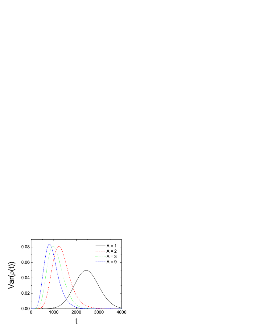
Figure 5: (Color online) Temporal behavior of the variance of the density of infected nodes in the LESFNs for different values of $A$. The results are obtained for $\lambda=0.001$ and on networks of size $N=10000$.

Since the intrinsic stochasticity of the epidemic spreading makes each realization unique [15, 17], it is valuable to analyze the statistical fluctuations around the average behavior for assessing simulation results with respect to real outbreaks. We measure the variance of the prevalence, defined by

$$Var(\rho(t))=E[(\rho(t)-\overline{\rho}(t))^{2}].$$ (3)

In order to evaluate this quantity, we have performed $500$ independent runs with different configurations of the intrinsic frequencies as well as different network realizations. Fig. 5 displays the time evolution of $Var(\rho(t))$ for LESFNs with different values of $A$. Since the initial prevalence is fixed and is the same for all instances, $Var(\rho(t))$ is initially equal to zero and can only increase. At very large time, almost all nodes are infected, implying that $\lim_{t\rightarrow\infty}Var(\rho(t))=0$. Compared with Fig. 3(b), one can easily find that time regions in which the fluctuations are maximal are the same as that in which the spreading velocities are the fastest. Moreover, an important feature is the rough symmetry of curves, regardless of $A=9$ (more randomly scale-free) or $A=1$ (more locally constrained) and the time regimes in which the fluctuations are maximal corresponding to a small diversity of the degrees of the infected nodes. This is also different from that in Barabási-Albert scale-free networks [15].

4 Conclusions

We have studied geographical effects on the spreading phenomena in lattice-embedded scale-free networks, in which a territory parameter $A$ controls the influence of the geographical structure on the network. We have investigated the temporal behavior of epidemic outbreaks and found that the spreading velocity reaches a peak very quickly in the initial infection period and then decays in an approximately exponential form in a more randomly scale-free region, which is consistent with previous studies. While the networks are more graphically constrained, this feature is apparently weakened. Furthermore, we have studied the propagation of the infection through different degree classes in the networks. Different from the clearly hierarchical dynamics in which the infection pervades the networks in a progressive cascade across smaller-degree classes in Barabási-Albert scale-free networks, epidemic smoothly spreads from higher- to lower-degree classes in the LESFNs. Finally, we have analyzed the prevalence fluctuations around the average epidemic process. A rough symmetry of curves is found and the time regions in which the fluctuations are maximal correspond to a small diversity of the degrees of the infected nodes, which is also different from that observed from Barabási-Albert scale-free networks.

5 Acknowledgements

X.-J. Xu acknowledges financial support from FCT (Portugal), Grant No. SFRH/BPD/30425/2006. G. Chen acknowledges the Hong Kong Research Grants Council for the CERG Grant CityU 1114/05E.

References

- [1] J.D. Murray, Mathematical Biology, Springer Verlag, Berlin, 1993; R.M. Anderson, R.M. May, Infectious Diseases in Humans, Oxford University Press, Oxford, 1992.
- [2] D.J. Watts, S.H. Strogatz, Nature 393 (1998) 440.
- [3] A.-L. Barabási, R. Albert, Science 286 (1999) 509; A.-L. Barabási, R. Albert, H. Jeong, Physica A 272 (1999) 173.
- [4] R. Albert, A.-L. Barabási, Rev. Mod. Phys. 74 (2002) 47; S.N. Dorogovtsev, J.F.F. Mendes, Adv. Phys. 51 (2002) 1079; M.E.J. Newman, SIAM Rev. 45 (2003) 167.
- [5] R. Cohen, K. Erez, D. ben-Avraham, S. Havlin, Phys. Rev. Lett. 85 (2000) 4626.
- [6] R.M. May, A.L. Lloyd, Phys. Rev. E 64 (2001) 066112.
- [7] M. Kuperman, G. Abramson, Phys. Rev. Lett. 86 (2001) 2909.
- [8] R. Pastor-Satorras, A. Vespignani, Phys. Rev. Lett. 86 (2001) 3200; Phys. Rev. E 63 (2001) 066117.
- [9] R. Cohen, S. Havlin, D. ben-Avraham, Phys. Rev. Lett. 91 (2003) 247901.
- [10] M. Barthélemy, A. Barrat, R. Pastor-Satorras, A. Vespignani, Phys. Rev. Lett. 92 (2004) 178101.
- [11] S.-H. Yook, H. Jeong, A.-L. Barabási, Proc. Natl. Acad. Sci. USA 99 (2002) 13382; G. Nemeth, G. Vattay, Phys. Rev. E 67 (2003) 036110; M.T. Gastner, M.E.J. Newman, Eur. Phys. J. B 49 (2006) 247.
- [12] A.F. Rozenfeld, R. Cohen, D. ben-Avraham, S. Havlin, Phys. Rev. Lett. 89 (2002) 218701; D. ben-Avraham, A.F. Rozenfeld, R. Cohen, S. Havlin, Physica A 330 (2003) 107.
- [13] C.P. Warren, L.M. Sander, I.M. Sokolov, Phys. Rev. E 66 (2002) 056105.
- [14] L. Huang, L. Yang, K. Yang, Phys. Rev. E. 73 (2006) 036102.
- [15] P. Crépey, F. Alvarez, M. Barthélemy, Phys. Rev. E 73 (2006) 046131.
- [16] M. Small, C.K. Tse, Physica A 351 (2005) 499; M. Small, C.K. Tse, D.M. Walker, Physica D 215 (2006) 146.
- [17] V. Colizza, A. Barrat, M. Barthélemy, A. Vespignani, Proc. Natl. Acad. Sci. USA 103 (2006) 2015.
- [18] M.E.J. Newman, S.H. Strogatz, D.J. Watts, Phys. Rev. E 64 (2001) 026118.
- [19] M. Barthélemy, A. Barrat, R. Pastor-Satorras, A. Vespignani, J. Theor. Biol. 235 (2005) 275.
- [20] Z.-X. Wu, X.-J. Xu, Y.-H. Wang, Eur. Phys. J. B 45 (2005) 385.