Interplay between function and structure in complex networks
Abstract
We show that abrupt structural transitions can arise in functionally optimal networks, driven by small changes in the level of transport congestion. Our results offer an explanation as to why so many diverse species of network structure arise in Nature (e.g. fungal systems) under essentially the same environmental conditions. Our findings are based on an exactly solvable model system which mimics a variety of biological and social networks. We then extend our analysis by introducing a novel renormalization scheme involving cost motifs, to describe analytically the average shortest path across multiple-ring-and-hub networks. As a consequence, we uncover a ‘skin effect’ whereby the structure of the inner multi-ring core can cease to play any role in terms of determining the average shortest path across the network.
PACS numbers: 87.23.Ge, 05.70.Jk, 64.60.Fr, 89.75.Hc
I Introduction
There is much interest in the structure of the complex networks which are observed throughout the natural, biological and social sciences newman ; newman2 ; watts98 ; nets ; nets2 ; charges ; central ; search ; gradient ; prl ; dm . The interplay between structure and function in complex networks has become a major research topic in physics, biology, informatics, and sociology watts98 ; nets ; nets2 ; charges ; central ; search ; gradient . For example, the very same links, nodes and hubs that help create short-cuts in space for transport may become congested due to increased traffic yielding an increase in transit time charges . Unfortunately there are very few analytic results available concerning network congestion and optimal pathways in real-world networks charges ; central ; search ; gradient ; danila ; moore ; gastner .
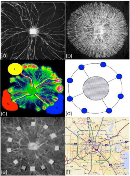
The physics community, in particular, hopes that a certain universality might exist among such networks. On the other hand, the biological community knows all too well that a wide diversity of structural forms can arise under very similar environmental conditions. In medicine, cancer tumors found growing in a given organ can have very different vascular networks. In plant biology, branching networks of plant roots or aerial shoots from different species can co-exist in very similar environments, yet look remarkably different in terms of their structure. Mycelial fungi mark provide a particularly good example, as can be seen in Figs. 1(a) and 1(b) which show different species of fungi forming networks with varying degrees of lateral connections (anastomoses). Not only do fungi represent a wide class of anastomosing, predominantly planar, transport networks, but they have close parallels in other domains, including vascular networks, road and rail transport systems, river networks and manufacturing supply chains. But given that such biological systems could adapt their structures over time in order to optimize their functional properties, why do we observe such different structures as shown in Figs. 1(a) and 1(b) under essentially the same environmental conditions?
In this paper, we provide exact analytic results for the effects of congestion costs in networks with a combined ring-and-star topology prl . We thus address the question above by showing that quite different network structures can indeed share very similar values of the functional characteristics relevant to growth. We also show that small changes in the level of network congestion can induce abrupt changes in the optimal network structure. In addition to the theoretical interest of such phase-like structural transitions, our results suggest that a natural diversity of network structures should arise under essentially the same environmental conditions – as is indeed observed for systems such as fungi (see Figs. 1(a) and (b)). We then extend this analysis by introducing a novel renormalization scheme involving cost motifs, to describe analytically the average shortest path across multiple-ring-and-hub networks. We note that although some of the findings of Ref. central appear similar to the present ones in terms of the wording of the conclusions, the context and structures considered are quite different – in addition, the results in the present paper are analytic and are obtained in a completely different way.
As a consequence of the present analysis, we uncover an interesting ‘skin effect’ whereby the structure of the inner multi-ring core can cease to play any functional role in terms of determining the average shortest path across the network. The implication is that any food that is found on the perimeter of the network structure, can be transported across the structure without having to go through the central core – and as a result, the network structure in the central core may begin to die out because of a lack of nutrient. Interestingly, there is experimental evidence that real fungal networks mark do indeed exhibit such a skin-effect. Other real-world examples in which an inner network core ceases to be fed by nutrients being supplied from the perimeter, and hence dies out, include the vasculature inside the necrotic (i.e. dead) region in a growing cancer tumour, and the inner core of a growing coral reef.
Our analytically-solvable model system is inspired by the transport properties of real fungi (see Fig. 1(c)). A primary functional property of an organism such as a fungus, is to distribute nutrients efficiently around its network structure in order to survive. Indeed, fungi need to transport food (carbon (C), nitrogen (N) and phosphorous (P)) efficiently from a localized source encountered on their perimeter across the structure to other parts of the organism. In the absence of any transport congestion effects, the average shortest path would be through the center – however the fungus faces the possibility of ‘food congestion’ in the central region since the mycelial tubes carrying the food do not have infinite capacity. Hence the organism must somehow ‘decide’ how many pathways to build to the center in order to ensure nutrients get passed across the structure in a reasonably short time. In other words, the fungus – either in real-time or as a result of evolutionary forces – chooses a particular connectivity to the central hub. But why should different fungi (Figs. 1(a) and (b)) choose such different solutions under essentially the same environmental conditions? Which one corresponds to the optimal structure? Here we will show that, surprisingly, various structurally distinct fungi can each be functionally optimal at the same time.
Figure 1(d) shows our model’s ring-and-hub structure. Although only mimicking the network geometry of naturally occurring fungi (Figs. 1(a) and (b)), it is actually a very realistic model for current experiments in both fungal and slime-mold systems. In particular, experiments have already been carried out with food-sources placed at peripheral nodes for fungi (Fig. 1(e)) and slime-mold slime with the resulting network structures showing a wide range of distinct and complex morphologies slime . We use the term ‘hub’ very generally, to describe a central portion of the network where many paths may pass but where significant transport delays might arise. Such delays represent an effective cost for passing through the hub. In practice, this delay may be due to (i) direct congestion at some central junction, or (ii) transport through some central portion which itself has a network structure (e.g. the inner ring of the Houston road network in Fig. 1(f)). We return to this point later on.
II The Model
II.1 The Dorogovtsev-Mendes model of a Small-World network
We begin by introducing the Dorogovtsev-Mendes (hereon DM) model dm of a small world network. The DM-model consists of a ring-hub structure, and places nodes around a ring, each connected to their nearest neighbour with a link of unit length. Links around the ring can either be directed in the “directed” model or undirected in the “undirected” model. With a probability each node is connected to the central hub by a link of length , and these links are undirected in both models.
We may proceed to solve this model, as in dm , by first finding the probability that the shortest path between any two nodes on the ring is , given that they are separated around the ring by length . These expressions can be found explicitly for both directed and undirected models. Summing over all for a given and dividing by yields the probability that the shortest path between two randomly selected nodes is of length . The average value for the shortest path across the network is then . For the undirected model, the expressions are more cumbersome due to the additional possible paths with equal length. However, if we define where and , a simple relationship may be found between the undirected and directed models in the limit with , that is . Thus the “directed” and “undirected” models only differ in this limit by a factor of two: , with now running from to .
II.2 The addition of congestion costs
We generalize the DM model of section II.1 to include a cost, , for passing through the central hubprl . This cost is expressed as an additional path-length, however it could also be expressed as a time delay or reduction in flow-rate for transport and supply-chain problems. We then consider a number of cases for the structure of such a cost, e.g. a constant cost where is independent of how many connections the hub already has, i.e. is independent of how ‘busy’ the hub is; a linear cost where grows linearly with the number of connections to the hub, and hence varies as ; or nonlinear cost where grows according to a number of nonlinear cost-functions.
For a general, non-zero cost that is independent of and , we can write (for a network with directed links):
| (1) | |||||
| (2) | |||||
| (3) |
Performing the summation gives:
| (4) |
The shortest path distribution is hence:
Using the same analysis for undirected links yields a simple relationship between the directed and undirected models. Introducing the variable with and as before, we may define and hence find in the limit , that . For a fixed cost, not dependent on network size or the connectivity, this analysis is straightforward. Paths of length are prevented from using the central hub, while for the distribution is similar to that of Ref. dm .
III Results for linear and quadratic cost-functions
For linear costs, dependent on network size and connectivity, we can show that there exists a minimum value of the average shortest path as a function of the connectivity to the central hub. We denote this minimal path length as . Such a minimum is in stark contrast to the case of zero cost per connection, where the value of would just decrease monotonically towards one with an increasing number of connections to the hub. The average shortest path can be calculated from from which we obtain
| (5) |
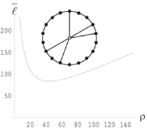
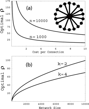
Figure 2 shows the functional form of with a cost of unit path-length per connection to the hub (i.e. , with ). The optimal number of connections in order that is a minimum is approximately and depends on . The corresponding minimal shortest path is approximately . Figure 3(a) shows analytic results for the optimal number of connections which yield the minimal shortest path , as a function of the cost per connection for a fixed network size. Figure 3(b) shows analytic results for the optimal number of connections which yield the minimal shortest path , as a function of the network size for a fixed cost per connection to the hub.
To gain some insight into the underlying physics, we make some approximations that will allow us to calculate the average shortest path analytically for a given cost-function that is valid within the approximations. We begin by noting that for large , or more importantly large , the first term in Eq. (III) may be written as . With the condition that the cost for using the hub isn’t too high, the region containing the minimum shortest path will be at sufficiently high to ignore this term, yielding a simplified form for the average shortest path:
| (6) |
We may then proceed by considering that, for a fixed network size and a cost that depends on connectivity, to locate the minima we differentiate Eq. (6) with respect to and set the result equal to zero and obtain
| (7) |
We substitute into this expression the scaled connectivity, , and it then becomes
| (8) |
In the limit of and , the dominant terms on both sides of Eq. (8) are those in leaving
| (9) |
From this expression we may obtain the location of the minimum of the average shortest path for a given cost-function for which the approximations are valid. For example, in the case of linear cost , we find that for the optimum number of connections we have . Using and , we obtain the value of the optimum number of connections as , which agrees well with the exact value calculated from Eq. (III). Inserting the optimum value for into Eq. (6) and keeping the largest terms we obtain , which also agrees well with the exact result.
We now consider quadratic cost-functions, . This could be a physically relevant cost-function when the cost for using the central hub depends on the number of connected pairs created, rather than the number of direct connections made to the hub. Solving for the optimal number of connections using Eq. (9) gives , corresponding to a minimum average shortest path length . One is also able to consider a cost dependant on a general exponent . This gives for the optimal number of connections
| (10) |
The corresponding average shortest path is a more complicated expression, but it scales with and as
| (11) |
This analysis can be adapted to the ‘undirected’ model by using the usual scaling relation between the models that was described above. For the case of linear costs on an undirected network one gets an optimal number of connections at and a minimum average shortest path of .

IV Results for non-linear cost-functions
We now consider the functional form of for non-linear cost functions, specifically a cubic cost-function and a ‘step’ cost-function. We show that for these non-linear cost-functions, a novel and highly non-trivial phase-transition can arise. First we consider the case of a general cubic cost-function:
| (12) |
where is the scaled probability, and . In order to demonstrate the richness of the phase transition and yet still keep a physically reasonable model, we choose the minimum in this cubic function to be a stationary point. Hence the cost-function remains a monotonically increasing function, but features a regime of intermediate connectivities over which congestion costs remain essentially flat (like the ‘fixed charge’ for London’s congestion zone). Since we are primarily concerned with an optimization problem, we can set the constant . Hence
| (13) |
where is the location of the stationary point. Substituting into Eq. (III) yields the shortest path distribution for this particular cost-function in terms of the parameters , , and . The result is too cumbersome to give explicitly – however we emphasize that it is straightforward to obtain, it is exact, and it allows various limiting cases to be analyzed analytically.
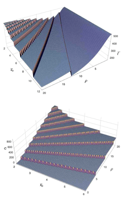
Figure 4 (top) shows the value of the average shortest path for varying values of and . As can be seen, the optimal network structure (i.e. the network whose connectivity is such that is a global minimum) changes abruptly from a high connectivity structure to a low connectivity one, as the cost-function parameter increases. Figure 4 (bottom) shows that this transition resembles a first-order phase transition. At the transition point , both the high and low connectivity structures are optimal. Hence there are two structurally inequivalent networks having identical (and optimal) functional properties. As we move below or above the transition point (i.e. or respectively) the high or low connectivity structure becomes increasingly superior.
Using the same approximations as those in Sec. III, we may estimate the approximate value of the cubic function parameter, , that will lead to two minima in the average shortest path distribution. We proceed by solving Eq. (9) with our cubic function as the cost-function:
| (14) |
The solutions to this equation are then stationary points in , and at least three stationary points are required for the distribution to have multiple minima. We thus have and . Inserting the central value, , into Eq. (14) gives an approximate lower bound for :
| (15) |
Although this calculation does not give us the value of , it is expected (and results confirm such a conjecture) to be close to . From this analysis, we can also see that both the location of the minima and the distance between them is governed by the cubic parameter .
We have checked that similar structural transitions can arise for higher-order nonlinear cost-functions. In particular we demonstrate here the extreme case of a ‘step’ function, where the cost is fixed until the connectivity to the central hub portion reaches a particular threshold value. As an illustration, we consider the particular case:
| (16) |
where depending on whether is negative, zero, or positive respectively, and determines the frequency of the jump in the cost. Figure 5 (top) shows the average shortest path for this step cost-function (Fig. 5 (bottom)) as and are varied. A multitude of structurally-distinct yet optimal network configurations emerge. As decreases, the step-size in the cost-function decreases and the cost-function itself begins to take on a linear form – accordingly, the behavior of tends towards that of a linear cost model with a single identifiable minimum. Most importantly, we can see that once again a gradual change in the cost parameter leads to an abrupt change in the structure of the optimal (i.e. minimum ) network.
V The ring-hub structure as a network motif
We have allowed our ring-and-hub networks to seek optimality by modifying their radial connectivity while maintaining a single ring. Relaxing this constraint to allow for transitions to multiple-ring structures yields a number of related findings. In particular, allowing both the radial connectivity and the number of rings to change yields abrupt transitions between optimal networks with different radial connectivities and different numbers of rings. One could, for example, consider this to be a model of a complicated fungal structure (Figs. 1(b), 1(e)) or of the interactions between hierarchies within an organization, such as in Fig. 6.
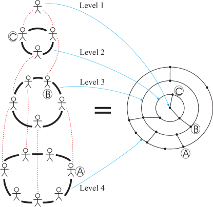
To analyze analytically such multiple-ring structures we introduce the following renormalization scheme. Consider the two-ring-and-hub network in Fig. 1(f). For paths which pass near the center, there is a contribution to the path-length resulting from the fact that the inner ring has a network structure which needs to be traversed. Hence the inner-ring-plus-hub portion acts as a renormalized hub for the outer ring. In short, the ring-plus-hub of Eq. (1) can be treated as a ‘cost motif’ for solving multiple-ring-and-hub problems, by allowing us to write a recurrence relation which relates the average shortest path in a network with rings to that for rings:
| (17) |
where and with being a general cost for the inner-most hub. The case is identical to Eq. (1). As before, represents the probability of a link between rings and and is the number of nodes in ring .
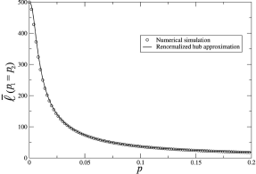
We investigate the properties of our renormalized -ring network by placing a number of constraints on the parameters and observing the average shortest path behaviour, so we may once again determine regimes of functionally optimal network configurations. We begin by increasing the number of rings to , with the constraint that the number of nodes on each ring is fixed. We find that the configuration that yields the minimum average shortest path length has all the ring probabilities, , equal. Figure 7 demonstrates the average shortest path distribution for such a case. Figure 7 also demonstrates the accuracy of our analytic renormalized result, as compared to a full-scale numerical calculation for . If we allow the number of nodes on the two rings to be different, we find that the configuration that optimizes the shortest path favours a larger number of connections on the ring with the most nodes. Returning to the original configuration, with an equivalent number of nodes on each ring, we consider the effect of a cost on the central hub of the inside ring. We find that a greater number of connections on the ring without costs optimizes the network, as one might expect.
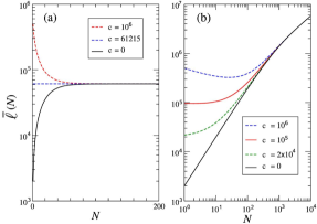
The addition of further rings, such that , leads to some interesting results. For a network with an equivalent number of nodes on each ring the optimal configuration remains such that all the ring probabilities, , are equal. However, for , we begin to see a deviation: connections should be moved to the outer rings of the network (those furthest away from the hub) in increasing numbers out to the edge of the network to obtain the minimum shortest path. We thus consider the properties of a network with varying ; equal ring probabilities ; inner ring costs, , that vary from ; both fixed numbers of nodes on each ring, constant, and varying numbers of nodes on each ring such that . Figure 8 shows the average shortest path distribution for several such cases. Interestingly, for large the system becomes indifferent to the cost of the central hub, , and all the distributions converge, in both the case of fixed and varying numbers of nodes on each individual ring. This is suggestive of an effective ‘skin effect’, as the center of the network becomes effectively disconnected after the addition of a large number of rings. The redundance of the central portion of the network offers an explanation for an earlier finding: that as we approach the optimal configuration ceases to be such that all innermost ring probabilities, , are equal. We find that to optimize the network we need to move the connections into the skin, more than likely as a result of the detachment of the center of the network from the whole.
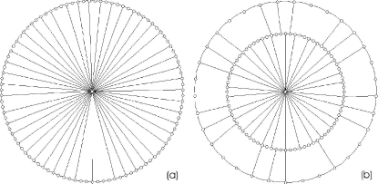
By comparison of the shortest path values of our multiple ring networks, we have found a further important result. We find that there are optimal network structures with different numbers of rings and radial connectivities, yet which have the same average shortest path length across them note . Hence, as before, optimal network structures exist which are structurally very different, yet functionally equivalent. Figure 9 shows an explicit example of two such functionally equivalent, optimal networks. It is remarkable that these images are so similar to the real fungi shown in Figs. 1(a) and (b).
VI Conclusion
In summary, we have analyzed the interplay between the structure and function within a class of biologically-motivated networks, and have uncovered a novel structural phase transition. Depending on the system of interest (e.g. fungus, or road networks) these transitions between inequivalent structures might be explored in real-time by adaptive re-wiring, or over successive generations through evolutionary forces or ‘experience’. Through the use of an approximation, we treated the original network as a cost-motif for a larger network and considered the circumstances under which such networks obtained their optimal functional structure. The equivalence in function, defined by the networks transport properties, between various topologically distinct structures may provide insight into the existence of such disparate structure in real fungi. An important further implication of this work is that in addition to searching for a universality in terms of network structure, one might fruitfully consider seeking universality in terms of network function.
Acknowledgements
We kindly acknowledge L. Boddy, J. Wells, M. Harris and G. Tordoff (University of Cardiff) for the fungal images in Figs. 1(a), (b) and (e). N.J. and M.F. acknowledge the support of EU through the MMCOMNET project, and N.J. acknowledges the support of the EPSRC through the Life Sciences Program.
References
- (1) M.E.J. Newman, SIAM Review 45, 167 (2003).
- (2) M.T. Gastner, M.E.J. Newman, cond-mat/0409702.
- (3) D.J. Watts and S.H. Strogatz, Nature 393, 440 (1998).
- (4) D. S. Callaway, M. E. J. Newman, S. H. Strogatz, and D. J. Watts, Phys. Rev. Lett. 85, 5468 (2000)
- (5) R. Albert and A.L. Barabasi, Phys. Rev. Lett. 85, 5234 (2000).
- (6) L.A. Brunstein, S.V. Buldyrev, R. Cohen, S. Havlin and H.E. Stanley, Phys. Rev. Lett. 91, 168701 (2003).
- (7) B. Danila, Y. Yu, S. Earl, J.A. Marsh, Z. Toroczkai and K.E. Bassler, cond-mat/0603861.
- (8) C. Moore, G. Ghoshal and M.E.J. Newman, cond-mat/0604069.
- (9) M.T. Gastner, and M.E.J. Newman, cond-mat/0603278.
- (10) R. Guimera, A. Diaz-Guilera et al., Phys. Rev. Lett. 89, 248701 (2002).
- (11) V. Colizza, J. R. Banavar et al., Phys. Rev. Lett. 92, 198701 (2004).
- (12) Z. Toroczkai, K. E. Bassler, Nature 428, 716 (2004).
- (13) D.J. Ashton, T.C. Jarrett, and N.F. Johnson, Phys. Rev. Lett. 94, 058701 (2005).
- (14) S.N. Dorogovtsev and J.F.F. Mendes, Europhys. Lett. 50, 1 (2000).
- (15) M. Tlalka, D. Hensman, P.R. Darrah, S.C. Watkinson and M.D. Fricker, New Phytologist 158, 325 (2003).
- (16) T. Nakagaki, R. Kobayashi, Y. Nishiura, and T. Ueda, Proc. R. Soc. Lond. B 271, 2305 (2004).
- (17) The networks need to be optimal in order that this question of equivalence be meaningful and non-trivial. By contrast, it is a fairly trivial exercise to find non-optimal structures which are functionally equivalent.