Scaling of Circulation in Buoyancy Generated Vortices

Abstract

The temporal evolution of the fluid circulation generated by a buoyancy force when two-dimensional (2D) arrays of 2D thermals are released into a quiescent incompressible fluid is studied through the results of numerous lattice Boltzmann simulations. It is observed that the circulation magnitude grows to a maximum value in a finite time. When both the maximum circulation and the time at which it occurs are non-dimensionalised by appropriately defined characteristic scales, it is shown that two simple Prandtl number (Pr) dependent scaling relations can be devised that fit these data very well over nine decades of Pr spanning the viscous and diffusive regimes and six decades of Rayleigh number (Ra) in the low Ra regime. Also, obtained analytically is the exact result that circulation magnitude continues to grow in time for a two-dimensional laminar or turbulent single buoyant (3D) vortex ring in an infinite unbounded fluid.

Buoyancy generated vorticity is an attractive area of study for its influential role in various fields of science and engineering, its relevance to mixing and, undoubtedly, for the aesthetically pleasing nature of its visualised flow structure (see, for example, Scorer (1957); Wilkins et al. (1971); Lupton et al. (1998); Brandenburg and Hazlehurst (2001); Zinn and Drummond (2005); Rogers and Morris (2005) and the references therein). Buoyant vortices are generated when plumes and thermals have different temperatures to an ambient fluid. Following some classical work on buoyant vortex rings and starting plumes Turner (1957, 1962), detailed studies on a single starting plume have generated some understanding, though not yet complete, of the interesting phenomena of mushroom-type vortex head generation and its pinch-off (see, for example, Pottebaum and Gharib (2004)). A number of studies on thermals have focused mainly on the time evolution of the linear dimension of the thermal and its penetration in the streamwise direction Lundgren et al. (1992); Thompson et al. (2000); Diez et al. (2003). Lundgren et al. Lundgren et al. (1992) has also provided some information on the time evolution of the circulation. Further, effects of the initial geometry of thermals on their evolution were investigated recently Shapiro and Kanak (2002); Bond and Johari (2005). Despite this considerable interest, some basic aspects of buoyancy generated vorticity remain to be elucidated, including the presence or otherwise of quantitative scaling laws in different flow regimes. Such scaling laws may be used to predict aspects of the behaviour of a system without performing full solutions of the system’s governing equations.

In this letter, the results of numerous computer simulations using the lattice Boltzmann method (LBM) are used to investigate the universal scaling behaviour associated with the circulation generated by buoyant forces when 2D thermals are released into a quiescent incompressible fluid. Also presented is an analytical derivation showing that for a 3D buoyant vortex ring formed by releasing a thermal in an infinite domain of a quiescent fluid the magnitude of the circulation grows continuously in time for both laminar and turbulent cases.

In terms of the Cartesian coordinate system ($x,y,z$) each of the simulated 2D systems comprised a $2L_{x}\times 2L_{y}\times 1$ sized domain of incompressible fluid which was initially quiescent and of uniform density, $\rho$, and temperature, $T_{0}$. The centre of the domain coincided with the origin of a Cartesian coordinate system. At time $t=0$ a circular (to within the lattice resolution) thermal of initial radius $R_{0}<L_{x},L_{y}$ and temperature $T_{1}<T_{0}$ was introduced into the centre of the domain. Cyclic boundary conditions were applied at all lattice boundaries making the simulation equivalent to that of an infinite system initialised with an infinite number of circular thermals positioned at the nodes of a rectangular array such that their centres were separated by $2L_{x}$ in the $x$-direction and $2L_{y}$ in the $y$-direction. The temperature difference causes the thermals to move in the negative (downward) $y$-direction which coincides with the direction of acceleration due to gravity $-g\,\hat{\mathbf{e}}_{y}$, where $\hat{\mathbf{e}}_{y}$ is the unit vector in the $y$-direction. This motion is caused by the buoyancy force acting on the thermal due to its density being different from that of the surrounding fluid. For $t>0$ the temperature of the thermal diffuses and convects as it descends and a vorticity field with non-zero component $\omega_{z}(x,y,t)\equiv\omega(x,y,t)=\nabla\wedge\mathbf{u}(x,y,t)=\partial_{x}u_{y}(x,y,t)-\partial_{y}u_{x}(x,y,t)$ is generated, where $u_{x}$ and $u_{y}$ are the fluid velocity components in the $x$ and $y$-directions, respectively. This system is governed by the Navier-Stokes equations with the Boussinesq approximation, written as

$$\partial_{i}u_{i} = 0,$$

$$D_{t}u_{i} = -\rho^{-1}\partial_{i}p-\delta_{iy}g+\alpha g\left(T-T_{0}\right)\delta_{iy}+\nu\partial_{j}^{2}u_{i},$$

and the equation for temperature field $T$

$$D_{t}T=\kappa\partial_{j}^{2}T,$$

where summation notation applies to the indices $i$ and $j$ which take the values $x$ and $y$, $D_{t}=\partial_{t}+u_{i}\partial_{i}$, $\delta_{ij}$ is the Kronecker delta function, $p$ is the pressure, $\nu$ is the kinematic viscosity and $\kappa$ is the thermal diffusivity. The solution of these equations with cyclic boundary conditions at $x=L_{x},-L_{x}$ and $y=L_{y},-L_{y}$ and initial temperatures $T_{1}$ and $T_{0}$ describes the flow field generated by the infinite rectangular array of thermals. It should be noted that $L_{x}\rightarrow\infty$ and $L_{y}\rightarrow\infty$ represents the situation of a single isolated thermal in an infinite fluid.

The LBM used to solve the governing equations was a multi-relaxation-time algorithm which sets all non-hydrodynamic modes to zero at each time step. It is based on the LBM for the Boussinesq equations described in Guo et al. (2002). At regular intervals during the simulations measurements were made of the circulation, $\Gamma(t)$, calculated over the $x>0$ half-domain and defined by $\Gamma(t)=\int_{-L_{y}}^{L_{y}}\int_{0}^{L_{x}}\omega(x,y,t)\,dx\,dy$. It was observed in all simulations that the circulation magnitude, $\Gamma(t)$, grew to a maximum value, denoted $\Gamma_{\textrm{max}}$, in a time denoted by $t_{\textrm{max}}$, and then decayed. The parameters influencing the phenomena are $g\alpha\Delta T$, $\nu$, $\kappa$, $R_{0}$, $L_{x}$ and $L_{y}$ (here, $\Delta T=\left|T_{0}-T_{1}\right|$). In general

$$\Gamma_{\textrm{max}} \equiv \Gamma_{\textrm{max}}\left(g\alpha\Delta T,\nu,\kappa,R_{0},L_{x},L_{y}\right),$$ (1)

$$t_{\textrm{max}} \equiv t_{\textrm{max}}\left(g\alpha\Delta T,\nu,\kappa,R_{0},L_{x},L_{y}\right).$$ (2)

To reveal the scaling relations for $\Gamma_{\textrm{max}}$ and $t_{\textrm{max}}$ a total of 211 individual simulations were performed using various combinations of the parameters $g\alpha\Delta T$, $\nu$, $\kappa$, $R_{0}$, $L_{x}$ and $L_{y}$. Sets of simulations were performed in which all variables except one were held constant and the values $\Gamma_{\textrm{max}}$ and $t_{\textrm{max}}$ were measured and recorded. The simulations were run for sufficient times, between $3,000$ and $160,000$ time steps depending on the parameter set, to enable the measurement of the initial growth of circulation and its subsequent decay. The parameter ranges, in lattice Boltzmann units, were as follows: $10^{-5}<\alpha g\Delta T<5\times 10^{-5}$, $10^{-4}<\nu<19/6$, $10^{-4}<\kappa<1$, $2/\sqrt{\pi}<R_{0}<4\sqrt{5/\pi}$, $30<L_{x}<500$ and $30<L_{y}<500$ . These dimensional parameters where combined to yield dimensionless parameters covering a wide range of values. Specifically: the Prandtl number, $\textrm{Pr}=\nu/\kappa$, ranged over nine decades ($10^{-4}<\textrm{Pr}<10^{4}$); the Rayleigh number, $\textrm{Ra}=g\alpha\Delta TR_{0}^{3}/\nu\kappa$, over six decades ($1.4\times 10^{-5}<\textrm{Ra}<38.5$); and the aspect ratios $\Lambda_{x}=L_{x}/R_{0}$ and $\Lambda_{y}=L_{y}/R_{0}$, over nearly two decades ($7.9<\Lambda_{x,y}<443$). The range of Pr crosses from the low to high (diffusive to viscous) Pr regimes; the range of Ra, however, remains in the low Ra regime.

Firstly, the dependency of the parameters $g\alpha\Delta T$, $R_{0}$, $L_{x}$ or $L_{y}$ was investigated by varying just one of these parameters and examining plots of $\Gamma_{\textrm{max}}$ and $t_{\textrm{max}}$ versus the varied parameter. This showed the following scaling relations to hold: $\Gamma_{\textrm{max}}\sim g\alpha\Delta T\sim R_{0}^{2}\sim L_{x}\sim L_{y}^{0}$ and $t_{\textrm{max}}\sim\left(g\alpha\Delta T\right)^{0}\sim R_{0}^{0}\sim L_{x}^{2}\sim L_{y}^{0}$. The dependency on $\nu$ or $\kappa$ was more complicated, as varying just one of these and examining plots of $\Gamma_{\textrm{max}}$ and $t_{\textrm{max}}$ versus the varied parameter showed behaviour that depended on Pr. These relations suggest appropriate characteristic scales for circulation and time are $\Gamma_{0}\equiv L_{x}R_{0}^{2}\,g\alpha\Delta T/\nu$ and $t_{0}\equiv L_{x}^{2}/\nu$, where the viscosity is used in the denominator to ensure the correct dimensionality ( note that one could have equally well used $\kappa$ instead of $\nu$). These characteristic scales, $\Gamma_{0}$ and $t_{0}$, thus contain the correct dependency of $\Gamma_{\textrm{max}}$ and $t_{\textrm{max}}$ on all the parameters except $\nu$ and $\kappa$. Along with (1) and (2), this suggests that the maximum circulation and the time of its occurrence may be written in the following dimensionless form which depends only on Pr

$$\Gamma_{\textrm{max}}/\Gamma_{0} = f_{1}\left(\textrm{Pr}\right),$$ (3)

$$t_{\textrm{max}}/t_{0} = f_{2}\left(\textrm{Pr}\right).$$ (4)

The functions $f_{1}\left(\textrm{Pr}\right)$ and $f_{2}\left(\textrm{Pr}\right)$ are as yet unknown, but, to see the scaling relations, $\Gamma_{\textrm{max}}/\Gamma_{0}$ and $t_{\textrm{max}}/t_{0}$ are plotted against Pr on log-log scales in Figure 1. The abscissa covers nine decades of Pr and the ordinate, about four decades of $\Gamma_{\textrm{max}}/\Gamma_{0}$ and $t_{\textrm{max}}/t_{0}$. The figures exhibit certain power laws which may be written as $\Gamma_{\textrm{max}}/\Gamma_{0}\propto\textrm{Pr}^{n}$ and $t_{\textrm{max}}/t_{0}\propto\textrm{Pr}^{m}$, where the values of $n$ and $m$ are observed to be different in different Pr regimes. The plots in Figure 1 suggest that the values of $n$ and $m$ tend to constant values in the limits of high and low Pr. Assuming this to be the case, the following scaling relations, chosen for their simple form and correct asymptotic behaviour, were fitted to the data

$$\Gamma_{\textrm{max}}/\Gamma_{0} = a\left(\textrm{Pr}^{-n_{l}}+\textrm{Pr}^{-n_{h}}\right)^{-1},$$ (5)

$$t_{\textrm{max}}/t_{0} = b\left(\textrm{Pr}^{-m_{l}}+\textrm{Pr}^{-m_{h}}\right)^{-1},$$ (6)

where $a$, $n_{l}$, $n_{h}$, $b$, $m_{l}$ and $m_{h}$ are constant fitting parameters. A nonlinear least-squares Marquardt-Levenberg algorithm was used to fit the data. The fitted scaling relations are shown as black lines on the plots in Figure 1 and it can be seen that they do indeed give extremely good fits to the data across all the Pr regimes. The fitted values of the fitting parameters are, with standard errors: $a=0.4936\pm 0.0046$, $n_{l}=0.9458\pm 0.0015$, $n_{h}=0.0539\pm 0.0014$, $b=0.20912\pm 0.0015$, $m_{l}=0.8770\pm 0.0013$ and $m_{h}=0.1275\pm 0.0012$. To within three standard errors all of these may be given as the following simple fractions: $a=1/2$, $n_{l}=19/20$, $n_{h}=1/20$, $b=7/34$, $m_{l}=7/8$ and $m_{h}=1/8$. It is an interesting observation, for which we have no explanation, that the fitted values suggest that $n_{l}=1-n_{h}$ and $m_{l}=1-m_{h}$. This suggests single exponent scalings of the form $\Gamma_{\textrm{max}}/\Gamma_{0}=a\,\textrm{Pr}^{n_{h}}\left(1+\textrm{Pr}^{2n_{h}-1}\right)^{-1}$ and $t_{\textrm{max}}/t_{0}=b\,\textrm{Pr}^{m_{h}}\left(1+\textrm{Pr}^{2m_{h}-1}\right)^{-1}$.

The dependencies on the other dimensionless parameters, Ra and the aspect ratio $\Lambda_{x}=L_{x}/R_{0}$, can be highlighted by writing the scalings relations (3) and (4) as $\Gamma_{\textrm{max}}/\kappa=\Lambda_{x}\textrm{Ra}\,f_{1}\left(\textrm{Pr}\right)$ and $\nu\,t_{\textrm{max}}/R_{0}^{2}=\Lambda_{x}^{2}\,f_{2}\left(\textrm{Pr}\right)$. The accuracy of scalings obtained for $\Gamma_{\textrm{max}}$ and $t_{\textrm{max}}$ are further confirmed by the plots in Figures 2 and 3 of the alternatively non-dimensionalised $\Gamma_{\textrm{max}}$ and $t_{\textrm{max}}$ plotted against the two dimensionless parameters Ra and $\Lambda_{x}$. In both figures the fitted scaling relations are shown as black lines, and again, the fits are seen to be extremely good.

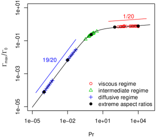
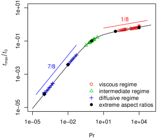
Figure 1: (Colour online) Dimensionless $\Gamma_{\textrm{max}}/\Gamma_{0}$ and $t_{\textrm{max}}/t_{0}$ plotted over six decades of Prandtl number. The black lines are the best fits to the functions using (5) and (6).

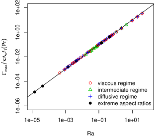
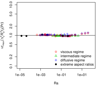
Figure 2: (Colour online) Particular non-dimensionalised forms of $\Gamma_{\textrm{max}}$ and $t_{\textrm{max}}$ plotted over six decades of Rayleigh number. The black lines are $\Gamma_{\textrm{max}}/\kappa\,\Lambda_{x}f_{1}\left(\textrm{Pr}\right)=\textrm{Ra}$ and $\nu\,t_{\textrm{max}}/\Lambda_{x}^{2}R_{0}^{2}f_{2}\left(\textrm{Pr}\right)=1$ respectively.

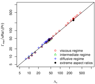
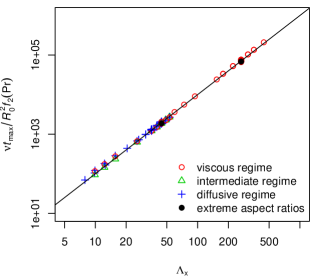
Figure 3: (Colour online) Particular non-dimensionalised forms of $\Gamma_{\textrm{max}}$ and $t_{\textrm{max}}$ plotted over two decades of the aspect ratio $\Lambda_{x}$. The black lines are $\Gamma_{\textrm{max}}/\kappa\,\textrm{Ra}\,f_{1}\left(\textrm{Pr}\right)=\Lambda_{x}$ and $\nu\,t_{\textrm{max}}/R_{0}^{2}\,f_{2}\left(\textrm{Pr}\right)=\Lambda_{x}^{2}$ respectively.

The scaling relations given in (5) and (6) suggest that in an infinite domain, that is to say, $L_{x}\rightarrow\infty$, $\Gamma_{\textrm{max}}$ and $t_{\textrm{max}}$ tend to infinity. A theoretical justification for this observation is now provided. The equation for the non-zero component of vorticity, $\omega$, can be written as

$$\partial_{t}\omega+\partial_{x}\left(u_{x}\omega\right)+\partial_{y}\left(u_{y}\omega\right)=\nu\left(\partial_{x}^{2}+\partial_{y}^{2}\right)\omega+\alpha g\partial_{x}T$$

and so the equation governing the circulation in an infinite domain can be written as

$$\partial_{t}\Gamma=\alpha g\int_{-\infty}^{\infty}\left(T_{0}-T|_{x=0}\right)dy-\nu\int_{-\infty}^{\infty}\left(\partial_{x}\omega|_{x=0}\right)\,dy.$$ (7)

The first term on the right-hand side (rhs) of (7) is the buoyancy term, which is always positive as $T_{0}>T_{1}$ forces $\left(T_{0}-T|_{x=0}\right)>0$. The second term on the rhs of (7) is negative due to the fact that $\partial_{x}\omega|_{x=0}\geq 0$ because of the change in the sign of $\omega$ near $x=0$. Also, the magnitude of this second term is zero at $t=0$ and starts to increase as the vorticity field is generated in the domain. In the limit of the viscous force being small compared to the buoyancy force, $\partial_{t}\Gamma$ remains positive and so $\Gamma$ will continue to increase without limit. Although the above argument for a continuous increase of $\Gamma$ requires $\nu$ to be small, this is not a restriction in the case of an axisymmetric buoyant vortex ring in an infinite domain as is now discussed.

Consider a domain of quiescent fluid of uniform density $\rho$ and temperature $T_{0}$ in a cylindrical coordinate system $(r,\theta,z)$ having $0\leq r\leq\infty$, $-\infty<z<\infty$ and $0\leq\theta<2\pi$ and acceleration due to gravity, $g$, acting in the negative $z$-direction. At time $t=0$ a spherical volume of fluid of radius $R_{0}$ and temperature $T_{1}<T_{0}$ is introduced into the domain with its centre coinciding with the origin of the coordinate system. For time $t>0$, the thermal starts descending along the $z$-axis due to the buoyancy force and a vortex ring of buoyant thermal fluid is generated (see, for example, Turner (1957) for a discussion of an ascending vortex ring when $T_{1}>T_{0}$). Due to the angular symmetry in the $\theta$-direction, this system can be analysed in 2D $(r,z)$ coordinates. By employing the Boussinesq approximation for the buoyancy force in the Navier-Stokes equations and using $\omega_{\theta}=\partial_{z}u_{r}-\partial_{r}u_{z}$ to denote the non-zero vorticity component, the governing equation for the circulation $\Gamma(t)=\int_{0}^{\infty}\int_{-\infty}^{\infty}\omega_{\theta}\,dz\,dr$ of the 2D vortex ring can be written as

$$\partial_{t}\Gamma=\alpha g\int_{-\infty}^{\infty}\left(T(r=0,z,t)-T_{0}\right)dz,$$ (8)

in which the viscous term does not arise due to the symmetry of the problem. Indeed, starting from the ensemble averaged (denoted by $\left\langle\cdot\right\rangle$) Navier-Stokes equations and applying various symmetry conditions to the ensemble averaged flow properties, one can show that $\partial_{t}\left\langle\Gamma\right\rangle=\alpha g\int_{-\infty}^{\infty}\left(\left\langle T(r=0,z,t)\right\rangle-T_{0}\right)dz$, where $\left\langle\Gamma\right\rangle=\int_{0}^{\infty}dr\int_{-\infty}^{\infty}dz\left\langle\omega_{\theta}\right\rangle$ is the ensemble average of the instantaneous circulation $\Gamma=\left\langle\Gamma\right\rangle+\Gamma^{\prime}$ and $\Gamma^{\prime}$ represents the turbulent fluctuations in $\Gamma$ over the $\left\langle\Gamma\right\rangle$. Thus, because $T(r=0,z,t)-T_{0}<0$, or $\left\langle T(r=0,z,t)\right\rangle-T_{0}<0$ for a turbulent system, (8) suggests that in the case of a descending vortex ring in an infinite domain both $\Gamma$ and $\left\langle\Gamma\right\rangle$ continue to decrease (or $\left|\Gamma\right|$ and $\left|\left\langle\Gamma\right\rangle\right|$ continue to increase) from their initial values of zero.

In this letter it was shown that, for an infinite system comprising an infinite number of 2D thermals initially arranged in a rectangular array, the magnitude of the buoyancy generated circulation, $\Gamma(t)$, reaches a maximum value, $\Gamma_{\textrm{max}}$, at a finite time, $t_{\textrm{max}}$. Accurate scaling relations for $\Gamma_{\textrm{max}}$ and $t_{\textrm{max}}$, covering nine decades of Pr and six decades of Ra, were inferred from LB simulations. Theoretical justification has been provided to support the observation, based on the scaling relations, that $\Gamma_{\textrm{max}}$ increases in proportion to the size of the domain. Furthermore, exact analytical results were derived for a single buoyancy generated vortex ring in both the laminar and turbulent cases. These exact results suggest that for a buoyant vortex ring in an infinite unbounded domain the magnitude of $\Gamma$, or $\left\langle\Gamma\right\rangle$ if the vortex ring is turbulent, will continue to grow indefinitely. The implication of this in predicting the growth of size $R$ of the vortex ring can be exhibited by the second term involving $d\Gamma/dt$ in $\pi\rho\Gamma\,dR^{2}/dt+\pi\rho R^{2}d\Gamma/dt=F_{b}$, where $F_{b}$ is constant buoyancy force acting on the buoyant fluid. In fact, Turner Turner (1957) assumed $\Gamma$ was constant and neglected this second term when predicting the growth of a vortex ring. We also note that it is assumed in the model used in Lundgren et al. (1992) that the circulation remains constant after an initial increase.

It is hoped that these results will inspire future work, for example: finding scaling relations and exponents in 3D cases with different initial configurations of thermals, addressing why the exponents found here add up to unity, and extending the study to examine high Ra regimes.

References

- Scorer (1957) R. S. Scorer, J. Fluid Mech. 2, 583 (1957).
- Wilkins et al. (1971) E. M. Wilkins, Y. Sasaki, and R. H. Schauss, Monthly Weather Review 99, 577 (1971).
- Lupton et al. (1998) J. E. Lupton, E. T. Baker, N. Garfield, G. J. Massoth, R. A. Feely, J. P. Cowen, R. R. Greene, and T. A. Rago, Science 280, 1052 (1998).
- Brandenburg and Hazlehurst (2001) A. Brandenburg and J. Hazlehurst, Astronomy and Astrophysics 370, 1092 (2001).
- Zinn and Drummond (2005) J. Zinn and J. Drummond, J. Geophys. Res. 110, A04306 (2005).
- Rogers and Morris (2005) M. C. Rogers and S. W. Morris, Phys. Rev. Lett. 95, 024505 (2005).
- Turner (1957) J. S. Turner, Proc. Royal Soc. London, Series A, Mathematical and Physical Sciences 239, 61 (1957).
- Turner (1962) J. S. Turner, J. Fluid Mech. 13, 356 (1962).
- Pottebaum and Gharib (2004) T. S. Pottebaum and M. Gharib, Experiments in Fluids 37, 87 (2004).
- Lundgren et al. (1992) T. S. Lundgren, J. Yao, and N. N. Mansour, J. Fluid Mech. 239, 461 (1992).
- Thompson et al. (2000) R. S. Thompson, W. H. Snyder, and J. C. Weil, J. Fluid Mech. 417, 127 (2000).
- Diez et al. (2003) F. J. Diez, R. Sangras, G. M. Faeth, and O. C. Kwon, J. Heat Trans. Trans. ASME 125, 821 (2003).
- Shapiro and Kanak (2002) A. Shapiro and K. N. Kanak, J. Atmos. Sci. 59, 2253 (2002).
- Bond and Johari (2005) D. Bond and H. Johari, Exp. in Fluids 30, 591 (2005).
- Guo et al. (2002) Z. Guo, B. Shi, and C. Zheng, International Journal for Numerical Methods in Fluids 39, 325 (2002).