Dependence of fluorescence-level statistics on bin time size in a few-atom magneto-optical trap

Abstract

We have analyzed the statistical distribution of the fluorescence signal levels in a magneto-optical trap containing a few atoms and observed that it strongly depends on the relative size of the bin time with respect to the trap decay time. We derived analytic expressions for the signal distributions in two limiting cases, long and short bin time limits, and found good agreement with numerical simulations performed regardless of the size of the bin time. We found an optimal size of the bin time for minimizing the probability of indeterminate atom numbers while providing accurate information on the instantaneous number of atoms in the trap. These theoretical results are compared with actual experimental data. We observed super-Poisson counting statistics for the fluorescence from trapped atoms, which might be attributed to uncorrelated motion of trapped atoms in the inhomogeneous magnetic field in the trap.

I INTRODUCTION

One of the long-sought experimental capabilities in modern atomic physics and quantum optics is the ability to load a single atom in a microscopic volume for an extended time and to manipulate and probe its internal and external states at will. In recent years, several groups have developed technics for trapping and controlling a single or a few neutral atoms based on tightly localized magneto-optical traps or dipole traps Ruschewitz96 ; Hu94 ; Haubrich96 ; Youn06 . Single or a-few-atom traps have been applied to wide range of fields such as cavity quantum electrodynamics studies Ye99 , experiments on single-photon generation on demand Barquie05 , and even archeological dating of ancient aquifers Sturchio04 .

The most distinctive signature of single atom trapping is the quantized fluorescence signal. When the number of trapped atoms is decreased to single-atom level, the fluorescence signal from atoms exhibits stepwise underlying variation in time and the size of the fluorescence signal with respect to a background level is interpreted as being proportional to the instantaneous number of atoms in the trap. Such stepwise fluorescence signals have been regarded as the most definitive evidence for single atom trapping. With this understanding, one can obtain the atom-number distribution in the trap from the histogram of the fluorescence signal levels and can also identify individual loading and loss events of atoms in the trap Youn06 ; Ueberholz00 .

In actual single-atom trap experiments, since the fluorescence signal from a single atom is extremely weak, one needs to choose a bin time for photon counting as long as possible in order to achieve enough signal to noise ratio. If the bin time is too long, however, the atom number can change several times during the bin time and thus the observed fluorescence no longer provides accurate information on the instantaneous atom number.

From the experimental point of view, therefore, several questions naturally arise regarding the conditions under which the fluorescence measurement should be performed: what will be the optimal size for the bin time, what determines the shape of the signal distribution and thus what information one can get from the observed signal distribution. The purpose of this paper is to answer these questions.

This paper is organized in the following way. In Sec. II, we define the problem and derive analytic expressions for the signal distributions in two limiting cases, long and short bin time limits, along with signal-to-noise considerations. These results are compared with numerical simulations in Sec. III, where an iterative method and Monte Carlo simulations are employed to calculate steady-state atom number distribution functions and the signal distributions regardless of the size of the bin time. In Sec. IV, an optimal size of the bin time is identified for minimizing the probability of indeterminate atom numbers while providing accurate information on the instantaneous number of atoms in the trap. The analytic expressions and numerical results are then compared with experimental results in Sec. V. It is demonstrated that the experimental signal distribution is well fit by our theoretical model and from observed signal distributions one can extract information not only on the number of atoms but also on the state of atoms in the trap. In Sec. VI, we summarize our findings and draw conclusions.

II Theoretical Consideration

In a few-atom trap, the fluorescence signal from atoms, induced by a probe laser or by a weak trap laser itself in the case of a magneto-optic trap (MOT), is proportional to the number of atoms in the trap. The fluorescence signal is measured with a photodetector, usually in photon counting mode with photon counting electronics. Suppose the signal counts are successively taken in time for a preset bin time of $\Delta t$. The signal counts $S_{i}$ measured in $i^{\rm th}$ time bin, specified as $t_{i}<t<t_{i+1}$ with $t_{i}\equiv i\Delta t$ ($i=0,1,2,\ldots$), can be written as

$$S_{i}=\int^{t_{i}+\Delta t}_{t_{i}}\left(\sum_{j=1}^{N(t)}a_{j}(t)+b(t)\right)dt\;,$$ (1)

where $N(t)$ is the instantaneous number of atoms in the trap ($N(t)=0,1,2,\ldots$), $a_{j}(t)$ is the counting rate of fluorescence from $j^{\rm th}$ atom, and $b(t)$ is the counting rate of background signal such as detector dark counts and scattered laser light or stray room light. The bin time $\Delta t$ is assumed to be much larger than spontaneous emission lifetime of atoms, typically tens of nanoseconds. The signal $S_{i}$ is truncated to the nearest integer by the counting electronics.

The instantaneous number of atoms $N(t)$ rapidly fluctuates due to various stochastic processes. Temporal change of its probability distribution function $P_{N}(t)$ is governed by the following master equation:

$$\frac{dP_{N}}{dt} = RP_{N-1}-\left[R+\Gamma_{1}N+\Gamma_{2}{N\choose 2}\right]P_{N}$$ (2)

$$+\Gamma_{1}(N+1)P_{N+1}+\Gamma_{2}{N+2\choose 2}P_{N+2}\;,$$

where $N=0,1,2,\ldots$ with $P_{-1}=0$, $R$ is loading rate of atoms into the trap, $\Gamma_{1}$ is the one-atom loss rate due to collisions with background gas, $\Gamma_{2}$ is the two-atom loss rate due to light-assisted intra-trap collisions Ueberholz00 . The master equation Eq.(2) cannot be solved analytically. However, for a microscopic trap with only a few atoms in a volume of a few micron in diameter, the two-atom loss terms proportional to $\Gamma_{2}$ are negligibly small, and thus approximate expressions for $P_{N}$ and the number correlation function $\left<N(t)N(t+\tau)\right>_{t}$ can be obtained Choi06 with $\left<~{}\right>_{t}$ denoting a time average. For now, we just neglect the two-atom loss terms. The analysis including these terms will be discussed later.

Without the $\Gamma_{2}$ terms, the master equation Eq.(2) becomes the same as the simple birth-death model of population 9 , yielding a Poisson distribution in steady state with a mean value $\bar{N}=R/\Gamma_{1}$ and a variance $\sigma^{2}=\bar{N}$. For a few-atom trap with $N\sim 1$, the correlation decay time $\tau$ of the number correlation function is given by $\tau=1/\Gamma_{1}$ and is the measure of the average time during which $N(t)$ remains constant Haubrich96 . When $\Gamma_{2}$ terms are not negligible, the correlation decay time is a complicate function of $R$, $\Gamma_{1}$ and $\Gamma_{2}$ and always smaller than $1/\Gamma_{1}$ due to the additional two-atom loss process Choi06 . We denote the correlation decay time in this case as $\tau_{\rm eff}$ in order to distinguish it from the above definition of $\tau$ for the $\Gamma_{2}=0$ case. The correlation decay time is also called the trap decay time for macroscopic traps.

The signal distribution shows much different behaviors depending on the size of $\Delta t$ with respect to $\tau$. For analytic analysis we consider two limiting cases, long bin time ($\Delta t\gg\tau$) and short bin time ($\Delta t\ll\tau$), as illustrated in Fig. 1. In the long bin time limit, there exist many loading and loss events in a single bin time whereas the atom number hardly changes during the bin time in the short bin time limit, and thus these two limiting cases lead to quite different signal distributions.

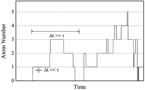
Figure 1: Number of atoms in the trap fluctuates in time due to stochastic processes. Two limiting cases of bin time, $\Delta t\gg\tau$ and $\Delta t\ll\tau$, for the integral in Eq. (1) are shown.

II.1 $\Delta t\gg\tau$ limit

Assume that $N\sim 1\ll a_{j}\Delta t,b\Delta t$ and that $a_{j}(t)$ and $b(t)$ fluctuate much faster than $\tau$. Under this assumption, for a given $N$ the variations in $a_{j}\Delta t$ and $b\Delta t$ go like square root of those, respectively, and thus much smaller than $a_{j}\Delta t$ and $b\Delta t$ themselves. On the other hand, the variation due to $N$ change is as large as $a_{j}\Delta t$. Therefore, in evaluating the integral in Eq. (1), we can neglect the fluctuations in $a_{j}$ and $b$ and replace them with their mean values $\bar{a}$ and $\bar{b}$, respectively.

$$S_{i}\simeq\int_{t_{i}}^{t_{i}+\Delta t}[N(t)\bar{a}+\bar{b}]dt=\left(N_{i}\bar{a}+\bar{b}\right)\Delta t\;,$$ (3)

where

$$N_{i}=\frac{1}{\Delta t}\int_{t_{i}}^{t_{i}+\Delta t}N(t)dt$$ (4)

is the time-averaged atom number in the $i^{\rm th}$ time bin. Since $\Delta t\gg\tau$, $N_{i}$, which is no longer an integer, fluctuates around the mean value $\bar{N}$ with a new variance $\tilde{\sigma}^{2}$, which is not the same as the variance $\sigma^{2}$ of $P_{N}$ distribution above. In fact, $\tilde{\sigma}^{2}\rightarrow 0$ as $\Delta t\rightarrow\infty$. The probability distribution $P(N_{i})$ can be obtained by the central limit theorem as a Gaussian distribution,

$$P(N_{i})=\frac{1}{\sqrt{2\pi}\tilde{\sigma}}\exp\left[-\frac{1}{2\tilde{\sigma}^{2}}(N_{i}-\bar{N})^{2}\right]\;,$$ (5)

where the variance $\tilde{\sigma}^{2}$ is proportional to the original variance $\sigma^{2}$, which equals $\bar{N}$ for a Poisson distribution, and inversely proportional to the sample size, which is in the order of $\Delta t/\tau$. The exact calculation for a Poisson distribution ($\Gamma_{2}=0$ case) is given below:

$$\tilde{\sigma}^{2} = \langle N_{i}^{2}\rangle-\langle N_{i}\rangle^{2}$$

$$= \frac{1}{\Delta t^{2}}\left<\int_{t_{i}}^{t_{i}+\Delta t}dt\int_{t_{i}}^{t_{i}+\Delta t}dt^{\prime}N(t)N(t^{\prime})\right>-\bar{N}^{2}$$

$$= \frac{1}{\Delta t^{2}}\int_{0}^{\Delta t}dt\int_{0}^{\Delta t}dt^{\prime}\left<N(t)N(t^{\prime})\right>_{t}-\bar{N}^{2}\;,$$

where $\langle~{}\rangle$ denotes an ensemble average and by the ergodic theorem the ensemble average is replaced with the time average. Since the correlation function for a Poisson distribution is given by 9

$$\langle N(t)N(t^{\prime})\rangle_{t}=\bar{N}^{2}+\bar{N}e^{-|t^{\prime}-t|/\tau}\;,$$ (7)

the variance becomes

$$\tilde{\sigma}^{2}=\frac{2\bar{N}\tau^{2}}{\Delta t^{2}}\left(e^{-\Delta t/\tau}+\Delta t/\tau-1\right)\;.$$ (8)

In the limit of $\Delta t\gg\tau$, we then obtain

$$\tilde{\sigma}^{2}\simeq 2\bar{N}\tau/\Delta t$$ (9)

as expected.

The probability distribution for $S_{i}$ is then obtained from Eqs. (3) and (5) as

$$P(S_{i})=\frac{1}{\sqrt{2\pi}\sigma_{S}}\exp\left[-\frac{1}{2\sigma_{S}^{2}}(S_{i}-\bar{S})^{2}\right]\;,$$ (10)

where

$$\bar{S}=(\bar{N}\bar{a}+\bar{b})\Delta t$$ (11)

and the deviation $\sigma_{S}$ is given by

$$\sigma_{S}=\tilde{\sigma}\bar{a}\Delta t\rightarrow\sqrt{2\bar{N}\bar{a}^{2}\tau\Delta t}$$ (12)

with the arrow indicating approximation under the condition of $\Delta t/\tau\rightarrow\infty$ and $\Gamma_{2}=0$. The signal to noise ratio $(S/N)_{S}$ for $S_{i}$ is given by

$$(S/N)_{S} \equiv \frac{\bar{S}}{\sigma_{S}}=\frac{(\bar{N}\bar{a}+\bar{b})}{\tilde{\sigma}\bar{a}}$$ (13)

$$\rightarrow [\bar{N}+\bar{b}/\bar{a}]\sqrt{\frac{\Delta t}{2\bar{N}\tau}}\propto\sqrt{\Delta t}\;,$$

increasing as the square root of the bin time. Fig. 2 shows the behavior of $P(S_{i})$ for different ratio of $\Delta t/\tau$. The distribution is single-peaked centered around $\bar{S}$ and the relative width of the peak with respect to the mean $\bar{S}$ becomes narrower as $\Delta t$ is made larger, as expected from Eq.(13).

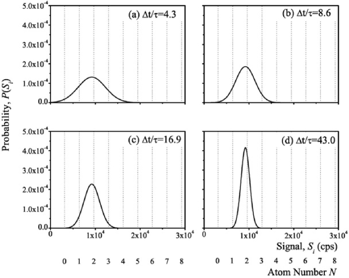
Figure 2: Signal distribution given by Eq. (10) with $\bar{N}$=1.9, $\bar{a}$=3270 s^-1, $\bar{b}$=3140 s^-1 and $\tau$=23 s. These parameters are derived from the experimental data in Ref. Choi06 . In plotting the distributions, signal counts are divided by corresponding bin times for the horizontal axis so as to align the distributions with different bin times. The dotted lines indicate corresponding atom numbers.

II.2 $\Delta t\ll\tau$ limit

In this limit, $N(t)$ remains at a certain integer value $m$ through out the bin time and thus

$$S_{i} = \int^{t_{i}+\Delta t}_{t_{i}}\left(\sum_{j=1}^{m}a_{j}(t)+b(t)\right)dt$$ (14)

$$= \sum_{j=1}^{m}A_{j,i}+B_{i}\;,$$

where

$$A_{j,i} = \int_{t_{i}}^{t_{i}+\Delta t}a_{j}(t)dt$$

$$B_{i} = \int_{t_{i}}^{t_{i}+\Delta t}b(t)dt$$ (15)

are the number of fluorescence and background counts in the bin time, respectively, and thus integers.

In general, the statistics of $A_{j,i}$ and $B_{i}$, with associated distribution functions $P_{a}(A_{j,i})$ and $P_{b}(B_{i})$, respectively, are not necessarily Poissonian. However, in many cases these quantities follow Poisson statistics. For example, although the photon statistics of resonance fluorescence of a small number of atoms is sub-Poissonian, when measured with an imperfect photodetector, the counting statistics become Poissonian. In addition, statistics of scattered light of laser beam is Poissonian. Of course, there are cases where these statistics become super-Poissonian, particularly when laser power fluctuations and other technical noises enter. For now, we just assume both $A_{j,i}$ and $B_{i}$ follow Poisson statistics with mean values $\bar{A}\equiv\bar{a}\Delta t$ and $\bar{B}\equiv\bar{b}\Delta t$, respectively.

Under this assumption, the conditional probability for $S_{i}$ with a constraint $N=m$ is given by

$$P(S_{i}|m)={\sum}^{\prime}_{\left\{A_{j,i},B_{i}\right\}}\left[\prod_{j=1}^{m}P_{a}(A_{j,i})\right]P_{b}(B_{i})$$ (16)

where ${\sum}^{\prime}_{\left\{A_{j,i},B_{i}\right\}}$ represents summations to be performed for all possible combinations of $A_{j,i}$ and $B_{i}$ under the constraint of Eq. (14). If we assume Poisson distributions for $P_{a}(A_{j,i})$ and $P_{b}(B_{i})$,

$$P(S_{i}|m) = {\sum}^{\prime}_{\left\{A_{j,i},B_{i}\right\}}\left[\prod_{j=1}^{m}\frac{\bar{A}^{A_{j,i}}e^{-\bar{A}}}{A_{j,i}!}\right]\frac{\bar{B}^{B_{i}}e^{-\bar{B}}}{B_{i}!}$$ (17)

$$= \frac{\left(e^{-\bar{A}}\right)^{m}e^{-\bar{B}}}{S_{i}!}{\sum}^{\prime}_{\left\{A_{j,i},B_{i}\right\}}S_{i}!\left[\prod_{j=1}^{m}\frac{\bar{A}^{A_{j,i}}}{A_{j,i}!}\right]\frac{\bar{B}^{B_{i}}}{B_{i}!}$$

$$= \frac{e^{-\bar{S}_{m}}}{S_{i}!}\left[\left(\sum_{j=1}^{m}\bar{A}\right)+\bar{B}\right]^{S_{i}}$$

$$= \frac{\bar{S}_{m}^{S_{i}}}{S_{i}!}e^{-\bar{S}_{m}}$$

where

$$\bar{S}_{m}=m\bar{A}+\bar{B}\;.$$ (18)

The resulting distribution is just a Poisson distribution with both mean value and variance equal to $\bar{S}_{m}$. For non-Poisson distributions for $P_{a}(A_{j,i})$ and $P_{b}(B_{i})$, the resulting $P(S_{i}|m)$ is not Poissonian. However, it is still a well-localized Gaussian-like distribution with a mean value $\bar{S}_{m}$, but its variance is no longer equal to $\bar{S}_{m}$.

The probability distribution for $S_{i}$ for all possible $N$ values is then given by

$$P(S_{i})=\sum_{m=0}^{\infty}P(S_{i}|N=m)\cdot P_{N=m}$$ (19)

where each $P(S|m)$, peaked around its mean $\bar{S}_{m}$ with a variance $\sigma_{m}^{2}$, is modulated by $P_{m}$ as shown in Fig. 3. The signal to noise ratio $(S/N)_{m}$ for the $N=m$ signal level becomes,

$$(S/N)_{m}=\sqrt{\bar{S}_{m}}=\sqrt{(m\bar{a}+\bar{b})\Delta t}\propto\sqrt{\Delta t}\;.$$ (20)

The half width of the $m$th peak in the signal distribution is also given by the square root of $\bar{S}_{m}$ and thus the ratio of the $m$th-peak full width to the spacing of two adjacent peaks is equal to

$$2\sqrt{\bar{S}_{m}}/\bar{A}=2\sqrt{\frac{m+\bar{b}/\bar{a}}{\bar{a}\Delta t}}\;.$$ (21)

Unless this ratio is very small, the adjacent peaks substantially overlap and thus we have a significant probability of indeterminate atom numbers. A necessary condition for well separated adjacent peaks is then $\tau\gg\Delta t\ggg 4/\bar{a}$.

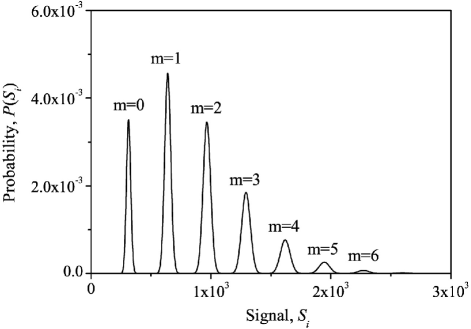
Figure 3: Signal distribution given by Eq. (19) with $\bar{N}$=1.9, $\bar{a}$=3270 s^-1, $\bar{b}$=3140 s^-1, $\tau$=23 s, $\Delta t$=0.100 s, and thus $\Delta t/\tau$=0.0043. These parameters are derived from the experimental data in Ref. Choi06 . Each peak in the distribution is marked with a corresponding atom number $m$.

For example, consider the set of parameters used in Figs. 2 and 3, $\bar{a}$=3270 s^-1, $\bar{b}$=3140 s^-1 and $\tau$=23 s, but with a very short bin time, $\Delta t/\tau$=0.00043. For these parameters the ratio in Eq. (21) is 0.34, 0.48, 0.59, 0.68 for $m=0,1,2,3$, respectively, and thereby results in significant overlap between adjacent peaks for $m\geq 1$. This situation is illustrated in Fig. 6(a), which is the result of Monte Carlo simulation obtained for this set of parameters. Detailed discussion on Fig. 6 will be given in the next section.

III Numerical Simulations

In the preceding sections, we argued that the two-atom loss terms in the master equation are negligibly small for a few-atom trap with a few-micron in size and thus the atom number distribution function is approximately Poissonian. When the number of atoms in such microscopic trap is increased with its size fixed, the two-atom loss processes take place more frequently. As a result, the atom-number distribution deviates significantly from a Poissonian distribution and thus the Poisson approximation in the preceding sections are no longer applicable. In this section, we include the two-atom loss term and calculate distribution functions numerically.

Although the master equation, Eq. (2), cannot be solved analytically, a steady-state solution can be found numerically. In steady state, we have $dP_{N}/dt=0$ and by rearranging terms we obtain the following recursion relation with $P_{-1}=0$.

$$RP_{N} = \frac{1}{2}(N+1)(2\Gamma_{1}+N\Gamma_{2})P_{N+1}$$ (22)

$$+\frac{1}{2}(N+2)(N+1)\Gamma_{2}P_{N+2}.$$

Using this relation the atom-number distribution $P_{N}$ can be easily calculated by iterative method. Alternatively, one can calculate a fluctuating time sequence of $S_{i}$ in steady state by simulating loading and one- and two-atom losses and simulating fluctuating $a_{j}(t)$ and $b(t)$ in Monte Carlo simulation. From the time sequence, one can calculate the histogram of atom number, i.e., the steady-state atom-number distribution.

We compare the results of these two numerical methods in Fig. 4. The values of $R,\Gamma_{1}$ and $\Gamma_{2}$ used in the calculations were derived from the experimental data of Ref. Choi06 . A Poisson distribution with the same $R$ and $\Gamma_{1}$ is also shown in Fig. 4 (by filled circle-line) for comparison. Once $P(N)$ is known, we can calculate the mean atom number $\bar{N}$ and variance $\sigma^{2}$. The results are $\bar{N}=1.6$ and $\sigma^{2}=1.5$, which should be compared with $\bar{N}=\sigma^{2}=R/\Gamma_{1}=1.9$ obtained for $\Gamma_{2}=0$. With inclusion of $\Gamma_{2}$ term, the mean atom number decreases because of the additional loss term. Although the distribution is not Poissonian, the deviation from a Poissonian distribution with the same $\bar{N}$ value is negligibly small. According to Ref.Choi06 , the correlation function which includes the two atom loss term can be approximated by the functional form for Poisson case as in Eq. (7) with $\tau$ replaced with an effective correlation decay time $\tau_{\rm eff}$.

$$\tau_{\rm eff}=1/\Gamma_{\rm eff}=4/[\Gamma_{1}+3\sqrt{\Gamma_{1}^{2}+4R\Gamma_{2}}]$$

For the above parameters, $\tau_{\rm eff}$=18 s, compared to $\tau=\Gamma_{1}^{-1}$=23 s.

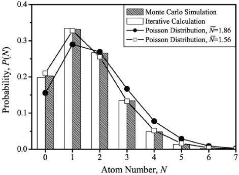
Figure 4: Atom number distribution for $R$=0.080 s^-1, $\Gamma_{1}$=0.043 s^-1 and $\Gamma_{2}$=0.0056 s^-1. For Monte Carlo simulation, we assumed $\Delta t$=0.20 s. Empty bar shows the probability calculated by iterative method and the filled bar that by Monte Carlo simulation. Filled circle-line shows a Poisson distribution with the same $R$ and $\Gamma_{1}$ but $\Gamma_{2}=0$ whereas empty square-line represents a Poisson distribution with the same mean value as the iterative and Monte Carlo simulations.

.

This observation allows us to use Eqs.(5) and (10) for the calculation of $P(N_{i})$ and $P(S_{i})$, respectively, with the $\bar{N}$ and $\tau_{\rm eff}$ values obtained above for nonzero $\Gamma_{2}$. For $\Delta t\ll\tau$ limit, we can calculate $P(S_{i})$ distribution by using Eq. (19) with substitution of the exact $P_{N=m}$ obtained numerically. In Fig. 5 the solid lines are given by Eqs. (10) and (19) and the filled area is by the Monte Carlo simulation.

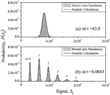
Figure 5: Signal distribution for $R$=0.080 s^-1, $\Gamma_{1}$=0.043 s^-1, $\Gamma_{2}$=0.0056 s^-1, $\bar{a}$=3270 s^-1 and $\bar{b}$=3140 s^-1. (a) $\Delta t\gg\tau$ limit, and (b) $\Delta t\ll\tau$ limit. Solid curves in (a) and (b) are obtained by Eq.(10) and Eq.(19), respectively, and filled areas are the result by Monte Carlo simulations in both cases. In (b), each peak is marked with a corresponding atom number.

The signal distribution $P(S_{i})$ in the intermediate region, other than two limiting cases considered above, can only be obtained by Monte Carlo simulations. From the time sequence of $S_{i}$ calculated by means of the Monte Carlo simulation with the aforementioned parameters, we can calculate $P(S_{i})$ for various $\Delta t/\tau$ by combining $S_{i}$ values in neighboring time bins. The results are summarized in Fig. 6. For $\Delta t/\tau\ll 1$, individual atom-number peaks are well separated and resolved as shown in Fig. 6(b) as long as $\Delta t/\tau\ggg 4/(\bar{a}\tau)$. Otherwise, the peaks for large $m$ overlap with neighboring peaks significantly as shown in Fig. 6(a). As the ratio $\Delta t/\tau$ increases, the broad background appears and grows in height as in Fig. 6(c) until the background outgrows the atom-number peaks completely as in Fig. 6(d).

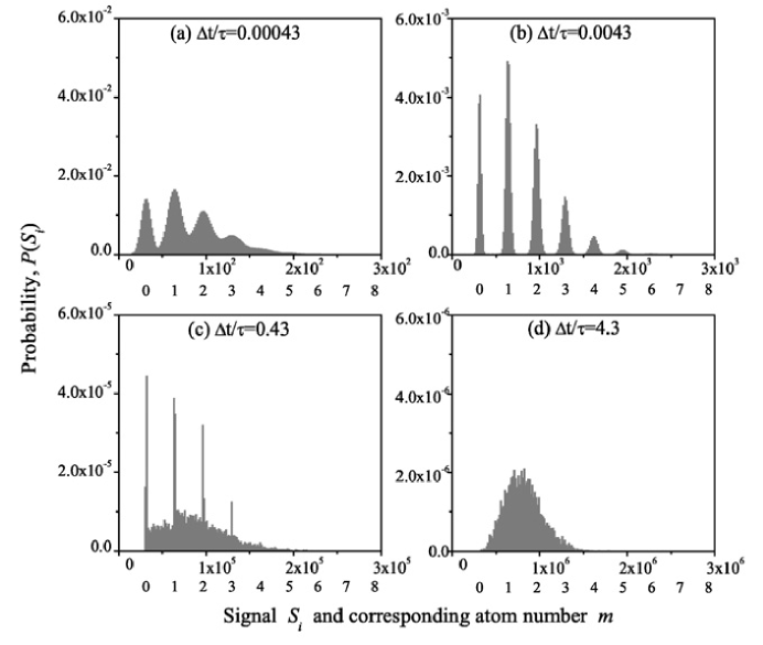
Figure 6: Dependence of signal distributions on $\Delta t/\tau$. (a), (b), (c) and (d) shows the results of Monte Carlo simulations.

IV Optimal Bin Time

The trend observed in Fig. 6 can be formulated in a quantitative way. We have observed for $\Delta t\ll\tau$ that individual signal distributions significantly overlap with neighboring peaks (due to poor signal-to-noise ratio) unless $\Delta t$ is much greater than $4/\bar{a}$. The overlap of distribution functions leads to an increase in the probability of having indeterminate atom numbers. We can quantify this probability ${\mathpzc P}_{<}$ as a sum of all areas under the distribution function $P(S_{i})$ outside the boundaries set by $\bar{S}_{m}-\eta\bar{A}<S_{i}<\bar{S}_{m}+\eta\bar{A}$ around the $m$th peak with $\eta<0.5$. In the time trace picture of fluorescence signal as in Fig. 7, this probability is proportional to the number of data points outside the region specified by dotted lines around a mean signal level. For these data points the atom number cannot be assigned unambiguously. From Eq. (19) we then obtain

$${\mathpzc P}_{<}(\Delta t)=\frac{1}{1-2\eta}\left[1-\sum^{\infty}_{m=0}\int^{\bar{S}_{m}+\eta\bar{A}}_{\bar{S}_{m}-\eta\bar{A}}P(S_{i})\ dS_{i}\right]$$ (23)

where the factor $1/(1-2\eta)$ is introduced in order to make $\mathpzc{P}_{<}$ be properly normalized in the limit of $\eta\rightarrow 0$.

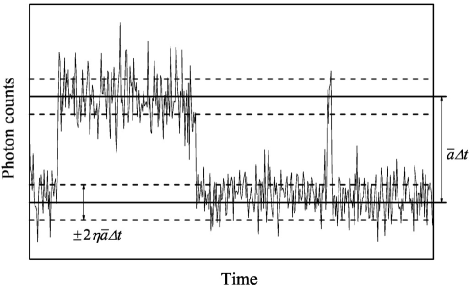
Figure 7: Signal counts outside a region centered around the mean signal level cannot be associated unambiguously with the atom number corresponding to the mean signal level.

The atom number also becomes indeterminate if it changes during the bin time as in the case of $\Delta t\gg\tau$. From the master equation, Eq. (2), it can be seen that the total rate of change $\Gamma_{\rm tot}$ of the atom number is given by

$$\Gamma_{\rm tot}(m)=R+\Gamma_{1}m+\Gamma_{2}{m\choose 2}.$$ (24)

for the atom number $m$ at that instance. The probability that the atom number would change from $N=m$ during $\Delta t$ is then

$${\mathpzc P}(\Delta t|N=m)=1-\exp[-\Gamma_{\rm tot}(m)\Delta t].$$ (25)

By summing over all possible atom numbers according to $P_{N}$, we obtain the probability ${\mathpzc P}_{>}(\Delta t)$ that the atom number would change during $\Delta t$ regardless of its initial values.

$${\mathpzc P}_{>}(\Delta t)=\sum^{\infty}_{N=0}\left\{1-\exp\left[-\Gamma_{\rm tot}(N)\Delta t\right]\right\}\cdot P_{N}.$$ (26)

If the atom number changes during the bin time $\Delta t$, the atom number cannot be determined unambiguously from the signal level for this particular bin time. Therefore, ${\mathpzc P}_{>}(\Delta t)$ can be regarded as the total probability of indeterminate atom numbers for $\Delta t\gtrsim\tau$.

In general, the above two processes occur independently and thus can occur simultaneous during $\Delta t$. Therefore, the total probability of indeterminate atom numbers for arbitrary $\Delta t$ is given by

$${\mathpzc P}_{\rm tot}(\Delta t)={\mathpzc P}_{>}(\Delta t)+{\mathpzc P}_{<}(\Delta t)-{\mathpzc P}_{>}(\Delta t)\cdot{\mathpzc P}_{<}(\Delta t).$$ (27)

In Fig. 8(a), this probability ${\mathpzc P}_{\rm tot}(\Delta t)$ is plotted as the ratio $\Delta t/\tau$ for several $\eta$ values. Symbols represent the results of Monte-Carlo simulations. The bin time $\Delta t$ that minimizes this probability can be regarded as an optimal bin time for accurate measurement of the instantaneous atom numbers in a few-atom trap. The optimal $\Delta t/\tau$ value is plotted as a function of $\eta$ in Fig. 8(b). It can be seen that for $0.2<\eta<0.4$ the optimal bin time is within the range of $0.003<\Delta t/\tau<0.008$. Particularly, for $\eta=0.3$, we have an optimal bin time of $\Delta t/\tau=0.004$ for the same parameter values as used in Figs. 2–6. Among the plots in Fig. 6, plot (b) is the most closest to the case of the optimal bin time.

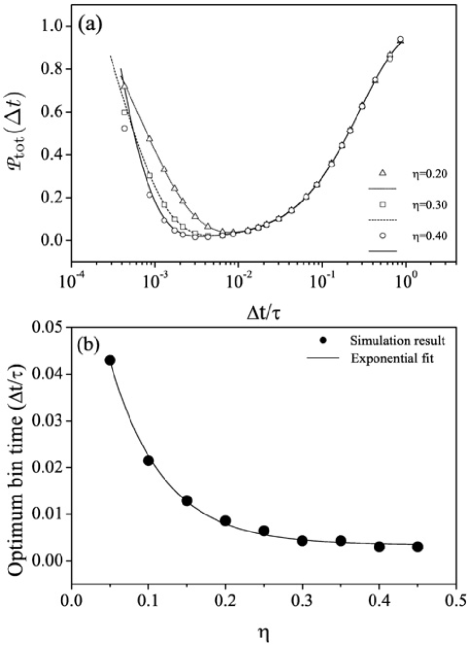
Figure 8: (a) Total probability ${\mathpzc P}_{\rm tot}(\Delta t)$ of indeterminate atom numbers, given by Eq. (27), for various values of $\eta$. Symbols denote Monte-Carlo simulation results. (b) Optimal bin time as a function of $\eta$.

V Comparison with Experimental Data

Detailed information on our experiment can be found elsewhere Youn06 ; Choi06 . In short, a few rubidium atoms were trapped in a microscopic MOT with a diameter of a few microns and fluorescence induced by a trap laser was measured in photon counting mode. A raw experimental data, a segment of which is shown in Fig. 9(a), was taken with a bin time of 0.20 s. The atom-number correlation time $\tau$ was measured to be 23 s, resulting in $\Delta t/\tau$ of 0.0086. Distributions with larger values of $\Delta t/\tau$ are derived from the raw data by combining counts in neighboring time bins.

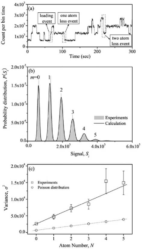
Figure 9: (a) A segment of the fluorescence signal time trace observed in the experiment in Ref. Choi06 . Loading events and atom- and two-atom loss events can be identified in the trace. (b) Signal distribution obtained from the experimental data in (a). The filled area shows the experimental result. The solid line shows a fit based on Eqs. (19) and (30). Each peak is marked with a corresponding atom number. (c) The filled squares represent the variances of individual atom-number peaks in the observed signal distribution in (b) whereas the unfilled squares show those of Poisson statistics. Bin time $\Delta t$ was 0.20 s and the correlation decay time $\tau$ was about 23 s in both experiment and analysis. All other parameter are the same as in Figs. 2–6.

We pay close attention to Fig. 9(b), where the fit is given by Eq. (19) with each $P(S_{i}|m)$ given by a Gaussian distribution with a mean of $\bar{S}_{m}=m{\bar{A}}+{\bar{B}}$ and a variance of $\sigma_{m}^{2}$ to be evaluated below.

The average background photon number, $\bar{B}=\bar{b}\Delta t$, and the average level spacing, $\bar{A}=\bar{a}\Delta t$, are 627 and 653, respectively, obtained from the experiment. By counting the individual loading and loss events in the time trace of fluorescence as shown in Fig. 9(a), one can measure the loading rate $R$ and the one- and two-atom loss rates $\Gamma_{1}$ and $\Gamma_{2}$, respectively, and the results are $R$=0.080 s^-1, $\Gamma_{1}$=0.043 s^-1, $\Gamma_{2}$=0.0056 s^-1. The detailed information on experiments to measure these rates can be found elsewhere Choi06 . From these parameters we obtain $\bar{N}$=1.6. The Poisson distribution for this actual $\bar{N}$ is used for $P_{N=m}$ in Eq. (19) for the fit. Note that the only fitting parameter is then the variance $\sigma_{m}^{2}$, which can be decomposed into

$$\sigma_{m}^{2}=\sigma_{B}^{2}+\sigma_{S}^{2}$$ (28)

where $\sigma_{B}^{2}$ and $\sigma_{S}^{2}$ are the variances of background and signal counts, respectively.

The background counts are mostly due to scattered light of trap and repump lasers of MOT. Due to long-term power fluctuations, the mean value of background counts also fluctuates, and as a result, the width of the zero-atom peak in the signal distribution $P(S_{i})$ becomes larger than that of a Poissonian distribution. In fact, the background variance $\sigma_{B}^{2}$ was measured to be 2570$\pm$180, about 4.5 times larger than the mean count $\bar{B}$.

If we assume that the fluorescence counts follow Poisson statistics, the variance $\sigma_{m}^{2}$ can be modeled as

$$\sigma_{m}^{2}=\sigma_{B}^{2}+m\sigma_{A}^{2}=(2570\pm 180)+m\bar{A}$$ (29)

where $\sigma_{A}^{2}$ is the variances of one-atom fluorescence, and it is assume that the fluorescence from one atom is statistically independent from that of another atom. However, as shown in Fig. 9(c), the observed variances of individual peaks are not well fit by the above formula. Rather they are well fit by an empirical formula given by

$$\sigma_{m}^{2}=(2570\pm 180)+(2280\pm 190)m\;,$$ (30)

the slope of which is about four times larger than that of Eq. (29).

The fact that the variance is still linear in $m$ indicates that the fluorescence from one atom is still statistically independent from that of another atom. This observation excludes, as a source of the increased variance, the fluorescence dispersion due to power fluctuation of trap and probe lasers, mechanical vibrations and similar technical noises since they all have to induce correlated fluctuations in the signals of individual atoms and thus proportional to $m^{2}$.

One possible reason for this increase variance is the motional effect of individual atoms. The atoms move independently from each other inside the MOT. Due to the spatially inhomogeneous magnetic field, atoms experience different Zeeman shifts and thus their upper level populations vary in time differently and independently from one atom to another. This variation can give rise to the observed increased variance in fluorescence counts.

Such motional effect might be observed in the second order correlation function of the fluorescence in the long time limit. In the short time limit, comparable to the life time of the atom (tens of nanosecond), antibunching characteristics of the resonance fluorescence will be dominant effect. But in the long time limit, much longer than the atomic life time and comparable to the characteristic time ($\sim$ millisecond) of atomic motion in the trap, an oscillatory feature would appear in the second order correlation function. The detailed study on this phenomena is beyond the scope of this paper and left for the future work.

VI Conclusion

We have derived analytic expressions for signal distribution $P(S_{i})$ of fluorescence photo-counts from a few-atom MOT and compared the results with Monte Carlo simulations and experimental data. The signal distribution strongly depends on the relative size of the bin time $\Delta t$ of photon counting with respect to the trap decay time $\tau$. In the limit of $\Delta t\ll\tau$, the distribution shows multiple peaks with the integrated areas of individual peaks constituting the atom-number distribution function $P_{N}$. Conversely, the stepwise fluorescence signal corresponding to a multi-peak distribution can be regarded as a definitive evidence of a few atoms in the trap. As $\Delta t\ll\tau$ is increased, a broad background appears and eventually outgrows sharp peaks corresponding to atom numbers and turns into a single peak in the limit of $\Delta t\gg\tau$. The validity of our derivation was confirmed by comparing the results with those of numerical simulations including Monte Carlo simulation. These theoretical results were then compared with experimental results. Fluorescence photo-count distributions were observed to be super-Poissonian, the origin of which might be due to the statistically independent motion of atoms in the inhomogeneous magnetic field of MOT. Our results provide necessary theoretical background for analyzing and interpreting the fluorescence signal of a few atom MOT and also clarify the optimum condition on the bin time in actual experiments.

This work was supported by National Research Laboratory Grants and Korea Research Foundation Grants (KRF-2002-070-C00044, -2005-070-C00058).

References

- (1) F. Ruschewitz, D. Bettermann, J. L. Peng and W. Ertmer, Europhys. Lett. 34, 651 (1996).
- (2) Z. Hu and H. J. Kimble, Opt. Lett. 19, 1888 (1994).
- (3) D. Haubrich, H. Schadwinkel, F. Strauch, B. Ueberholz, R. Wynands and D. Meschede, Europhys. Lett. 34, 663 (1996).
- (4) S. Yoon, Y. Choi, S. Park, J. Kim, J.-H. Lee, and K. An, Appl. Phys. Lett. 88, 211104 (2006).
- (5) J. Ye, D. W. Vernooy and H. J. Kimble, Phys. Rev. Lett. 83, 4987 (1999).
- (6) B. Darquié, M. P. A. Jones, J. Dingjan, J. Beugnon, S. Bergamini, Y. Sortais, G. Messin, A. Browaeys, and P. Grangier, Science 309, 454 (2005).
- (7) N. C. Sturchio, X. Du, R. Purtschert, B. E. Lehmann, M. Sultan, L. J. Patterson, Z.-T. Lu, P. Muller, T. Bigler, K. Bailey, T. P. O’Connor, L. Young, R. Lorenzo, R. Becker, Z. El Alfy, B. El Kaliouby, Y. Dawood and A. M. A. Abdallah, Geophys. Res. Lett. 31, L05503 (2004).
- (8) B. Ueberholz, S. Kuhr, D. Frese, D. Meschede and V. Gomer, J. Phys. B: At. Mol. Opt. Phys. 33, L135-L142 (2000).
- (9) Y. Choi, S. Yoon, S. Kang, W. Kim, J. Lee and K. An, “Analysis of the atom-number correlation function in a few-atom trap”, arxiv:physics/0604220.
- (10) C. W. Gardiner, Handbook of Stochastic Methods (Springer-Verlag, Berlin, 1983).