Scaling laws for the tropical cyclone derived from the stationary atmospheric vortex equation

Abstract

In a two-dimensional model of the planetary atmosphere the compressible convective flow of vorticity represents a strong nonlinearity able to drive the fluid toward a quasi-coherent vortical pattern. This is similar to the highly organised motion generated at relaxation in ideal Euler fluids. The problem of the atmosphere is however fundamentally different since now there is an intrinsic length, the Rossby radius. Within the Charney Hasegawa Mima model it has been derived a differential equation governing the stationary, two-dimensional, highly organised vortical flows in the planetary atmosphere. We present results of a numerical study of this differential equation. The most characteristic solution shows a strong similarity with the morphology of a tropical cyclone. Quantitative comparisons are also favorable and several relationships can be derived connecting the characteristic physical parameters of the tropical cyclone: the radius of the eye-wall, the maximum azimuthal velocity and the radial extension of the vortex.

1 Introduction

In the absence of dissipation the two-dimensional models of the planetary atmosphere and of the magnetized plasma can be reduced to differential equations having the same structure: the Charney equation for the nonlinear Rossby waves, in the physics of the atmosphere (Charney 1948); and the Hasegawa-Mima equation for drift wave turbulence, in plasma physics (Hesagawa and Mima 1978). One of the characteristics of these equations is the presence of an intrinsic length parameter, which can be seen from the fact that there is no space scale invariance, in contrast to the Euler equation (see Horton and Hasegawa 1994). This length is the Rossby radius for the atmosphere and the ion sonic Larmor radius for the magnetized plasma.

A long series of observations, experiments and theoretical (analytical and numerical) studies has established that the fluids exhibit an intrinsic trend to organisation. This is most obvious at relaxation from turbulent states when the fluid evolves toward a reduced subset of flow patterns, characterized by regular form of the streamfunction as shown for example by Mathaeus et al. 1991a, Matthaeus et al. 1991b, Kinney et al. 1995, Horton and Hasegawa 1994 (and references therein).

It has been shown (Spineanu and Vlad 2005) that the stationary states attained at late times in the evolution of the Charney-Hasegawa-Mima (CHM) fluids are described by the following equation

$$\Delta\psi+\frac{1}{2p^{2}}\sinh\psi\left(\cosh\psi-p\right)=0$$ (1)

Here $\psi$ is the streamfunction and $p$ is a positive constant. This equation has been derived within a field-theoretical formulation of the model of interacting point-like vortices and reveals that the asymptotic state of organization of the physical vorticity in fluids and plasmas is identical to states of self-duality of classical field theory of matter interacting with a gauge field. Consistent with the physical model from which it is derived, this equation should describe the states of fluids/plasmas characterized by the presence of a background of vorticity (a condensate of vorticity) and a finite intrinsic length (or a velocity of propagation of perturbation, like the gravity wave speed or the sonic speed). The numerical solutions of this differential equation has provided interesting results for the physical systems which it should be able to describe: plasma vortices, atmospheric vortices, non-neutral plasma vortex crystals, current sheets. Comparisons with experimental results on Navier-Stokes fluid, consisting of scatterplots $\left(\psi,\omega\right)$ $\equiv$ (streamfunction, vorticity) (de Rooij et al. 1999), and with the scatterplots obtained in numerical simulations by Seyler (1995) are also favorable. A brief discussion of the derivation of Eq.(1) will be presented in Section 2.

Due to the similar analytical structure (although for largely different magnitude of parameters) of the plasma vortex and the atmospheric vortex, we expect that this equation leads to solutions that may capture the strong nonlinear character of the atmospheric vortical flows in those states where the stationarity can be assumed a good approximation. Certainly the problem of the structure of the atmospheric vortex cannot be reduced in general to only fluid nonlinear dynamics, knowing the very important role of the heat exchange and moisture transport and condensation processes. These are essential elements of tropical cyclogenesis (see Emanuel 1986 and 1989 and references therein) but it is often accepted that the fluid dynamics is an adequate framework to study the vortex structure at the late stage of the evolution (Reasor and Montgomery 2001, Kossin and Schubert 2001). The fluid dynamic nonlinearity becomes the dominant constraint determining the structure of the velocity field when the thermodynamic processes have reached the stationary equilibrium.

The results of a numerical investigation of equation (1), for a range of parameters relevant for the physics of the atmosphere, are summarised here.

The monopolar solutions of the differential equation have the same morphology as the two-dimensional flow of a tropical cyclone (Willoughby and Black 1996, Wang and Wu 2004, Reasor and Montgomery 2001, Kossin and Schubert 2001). The solutions are characterized by a very narrow dip of the profile of the azimuthal velocity (tangential wind) in the center of the vortex. The radius of the “maximum tangential wind” or the radius of the eye wall is much smaller than the radius of the vortex. There is a decay of the magnitude of the azimuthal velocity toward the periphery, which is much slower compared with the fast decay toward the center. We find a very low magnitude (almost vanishing) of the vorticity over most of the vortex (approx. from the radius of maximum wind to the periphery), while the magnitude in a narrow central region is extremely high. Quantitatively, we obtain for the diameter of the cyclone’s eye a magnitude which compares well with the observations. The maximum vorticity is in a realistic range and the radial profile of the tangential velocity is similar to what is found in observations or with what is obtained in empirical models and numerical simulations. These favorable comparisons are valid in the case of mature, quasi-stationary tropical cyclones, after the phases of genesis and dynamic intensification.

Besides the structure of the flow, the numerical solutions for a very large number of cases provide a large data set from which various correlations can be extracted. In this regard we are mainly led to look for correlations between parameters that may present interest in practical cases and eventually can be compared with the observations. The main parameters that have been collected in the numerical work are: total radial extension of the atmospheric vortex, $R_{\max}$; the radius where the maximum of the tangential velocity is attained, $r_{v_{\theta}^{\max}}$; the magnitude of the maximum tangential wind, $v_{\theta}^{\max}$. In addition we have collected the total energy $E_{fin}$ and vorticity $\Omega_{fin}$ in the final state flow field. It is encouraging that we find the linear relationship, $E_{fin}\sim\Omega_{fin}$ which has also been revealed in numerical investigations of a large ensemble of point-like vortices (Yatsuyanagi et al. 2005). The numerical studies carried out until now are organized in the form of several scaling relations connecting vortex characteristics to the few parameters of the Eq.(1). They may be used for comparison with observation or with more complex theoretical models.

In addition, the numerical study of Eq.(1) reveals the existence of metastable states (quasi-solutions) consisting of (a) extremely concentrated vortical flows, similar to the cross section of a tornado and (b) collection of vortices with symmetric positions in plane (vortex crystals).

2 The physical model and the field theoretical description

In this section we briefly recall the origin of Eq.(1). It is useful to consider first the ideal fluid described by the Euler equation, for which it has been shown that it evolves at relaxation toward a very ordered flow pattern, consisting of two (positive and negative) vortices. This state persists for long times, being limitted by only the effect of some residual dissipation. From numerical simulations it has also been inferred the form of the flow function. It has been found that the streamfunction $\psi\left(x,y\right)$ obeys, in these states, the sinh-Poisson equation, an equation which has very special properties. It is an exactly integrable equation (by Inverse Scattering Transform) and is connected with a wide class of fundamental systems, like the Thirring lattice of spins in plane, the affine Toda system, the Gauss-Codazzi equations for embedding a surface in three dimensional space, etc. David Montgomery and his collaborators have developed a theoretical statistical model which explains the presence of this equation in this context (Kraichnan and Montgomery 1980, Fyfe, Montgomery and Joyce 1976, Joyce and Montgomery 1973, Montgomery and Joyce 1974, Montgomery et al. 1992).

The Euler equation is

$$\left[\frac{\partial}{\partial t}+\left(-\mathbf{\nabla}_{\perp}\psi\times\widehat{\mathbf{n}}\right)\cdot\mathbf{\nabla}_{\perp}\right]\mathbf{\omega}=0$$ (2)

where $\widehat{\mathbf{n}}$ is the versor perpendicular on the plane, the velocity and the vorticity are respectively $\mathbf{v}=-\mathbf{\nabla}_{\perp}\psi\times\widehat{\mathbf{n}}$ and $\mathbf{\omega}=\widehat{\mathbf{n}}\mathbf{\nabla}_{\perp}^{2}\psi$. It is generally accepted (but not yet mathematically proved) that the Euler fluid may be described by an equivalent model, consisting of a set of discrete point-like vortices moving in plane under the effect of mutual interaction. The latter is expressed by a potential given by the natural logarithm of the relative distance between vortices normalized to the linear extension of the region in plane where the motion is bounded (Kraichnan and Montgomery 1980). A fundamental observation is that this formulation exhibits a particular structure: matter, field, interaction. The matter corresponds to the density of point-like vortices in plane; the field is derived from the potantial and can be seen as an independent component of the system; the interaction appears as the usual combination of the matter current with the potential and leads to the equation of motion of the point-like vortices. The sinh-Poisson equation has been derived by formulating the continuum version of the point-like vortices model as a field theoretical model of interacting gauge and matter fields in the adjoint representation of $SU\left(2\right)$ (Spineanu and Vlad 2003). The essential point of the latter derivation was the self-duality of the relaxation states of the fluid.

In its simplest form the Charney-Hasegawa-Mima equation is

$$\frac{\partial}{\partial t}\left(1-\mathbf{\nabla}_{\perp}^{2}\right)\psi-\left[\left(-\mathbf{\nabla}_{\perp}\psi\times\widehat{\mathbf{n}}\right)\cdot\mathbf{\nabla}_{\perp}\right]\mathbf{\nabla}_{\perp}^{2}\psi=0$$ (3)

Similar to the Euler equation there is a discrete vortex model for the Charney-Hasegawa-Mima equation, where the potential of interaction is now short range (the modified Bessel function of zero order), i.e. it decays on the range given by the intrinsic length of the CHM equation. This model has been used in meteorology by Morikawa (Morikawa 1960) and Stewart (Stewart 1943).

In a similar approach as for the Euler fluid, it has been developed (Spineanu and Vlad 2005) a field theoretical model for the continuous version of the point-like vortices with short range interaction, based on the Chern-Simons action for the gauge field in interaction with the nonlinear matter field, in the adjoint representation of the $SU\left(2\right)$ algebra. In this model it is possible to derive the energy as a functional that becomes extremum on a subset of stationary states and presents particular properties. The general characterization of this family of states is their self-duality, which here means that the energy functional becomes minimum when the squared terms in its expression are all vanishing, leaving as lower bound for energy a quantity with topological meaning, proportional with the total vorticity.

The result is a set of equations parametrized by the solutions of the Laplace equation in two-dimensions. The Eq.(1) is the simplest of this family.

3 Numerical studies

To solve Eq.(1) we use the code “GIANT A software package for the numerical solution of very large systems of highly nonlinear systems” written by U. Nowak and L. Weimann (Nowak and Weiman 1990). The code is part of the numerical software library CodeLib of the Konrad Zuse Zentrum fur Informationstechnik Berlin. The meaning of the abbreviation is: GIANT = Global Inexact Affine Invariant Newton Techniques. This code solves nonlinear problems

$$F\left(\psi\right) = 0$$ (4)

$$\text{initial guess of solution, }\psi = \psi^{\left(0\right)}$$

where $F\left(\psi\right)$ is a nonlinear partial differential operator. The presence of the hyperbolic trigonometric functions, with very fast variation with the argument, renders the equation difficult to solve and many initial conditions do not lead to a solution since they cannot initiate a converging iteration. With all the difficulties of finding a right initialization of the integration procedure we note however that the solution with the morphology of a tropical cyclone appears insistently from a wide class of initial functions which contains vortical flows.

3.1 Parameters and Initializations

Eq.(1) has been derived from the self-duality subset of the Euler-Lagrange variational equations for the action functional of the field-theoretical model. In this action there are only two physical parameters: the coefficient of the Chern-Simons action, which we have identified as the sound speed, $c_{s}$ and the asymptotic vorticity which is the Coriolis frequency $f_{0}$ (or, in plasma physics, the ion cyclotron frequency $\Omega_{c}$). The space-like parameter that normalizes the Laplace operator in the Eq.(1) is the ratio

$$\rho_{g}=c_{s}/f_{0}$$ (5)

i.e. the Rossby radius $\rho_{g}$ (respectively the sonic Larmor radius in plasma, $\rho_{s}=c_{s}/\Omega_{ci}$). All distances implied in the solution are normalized to $\rho_{g}$. The streamfunction is normalised as

$$\psi=\frac{\psi^{phys}}{\rho_{g}^{2}f_{0}}$$ (6)

The unit for the streamfunction is $\rho_{g}^{2}f_{0}$ and the unit for vorticity $f_{0}$. Then the unit for velocity is $\rho_{g}f_{0}$. Here and in the rest of the paper the upperscript phys is used to indicate that the quantity is dimensional, measured in appropriate physical units. However the units themselves (i.e. $\rho_{g}$, $f_{0}$ and combinations) are written without this upperscript since there can be no confusion.

If we know the large radial extension of a vortex ($R_{\max}^{phys}$) the normalized parameter $R_{\max}$ is obtained by dividing to $\rho_{g}$. The result of integration is very sensitive to $R_{\max}$ and this points out the essential role played by $\rho_{g}$ in numerical studies aiming to reproduce observations. When the depth of the atmospheric perturbation is $H$, the Rossby radius is $\rho_{g}=\left(gH\right)^{1/2}/f_{0}$ (where $g$ is the gravitational acceleration). Actually $\rho_{g}$ is influenced by several other parameters than $H$, in particular the vorticity and it can have a range from tens to thousand kilometers. When combined with the range of vortex extensions $R_{\max}^{phys}$, it results that $R_{\max}$ has a range between a fraction of unity to few units (in plasma $R_{\max}$ can be hundreads to thousands). For mature stationary cyclones the radial extension of the cyclon vortex and the Rossby radius are of similar magnitude and this means that we have to study the range $R_{\max}\sim 1$.

The domain of integration is a square with a side of length $2L$

$$\left(x,y\right)\in\left[-L,L\right]\times\left[-L,L\right]$$ (7)

on which we place a rectangular mesh $n\times n$ usually with $n=101$.

We impose Dirichlet boundary conditions i.e. the streamfunction is a constant, $\psi_{b}$ on the limits of the square of integration. Here $\psi_{b}$ is the smaller root of the equation $\cosh\psi-p=0$ and since in all our runs we have $p=1$, the condition is $\psi_{b}=0$. This means zero vorticity at the boundary but it has defavorable effect on the velocity field, which does not allways vanish at the border.

In general the initial profiles have been of various types: (a) symmetric profiles (e.g. Gaussian functions, or various annular shapes) with maximum centered on $\left(0,0\right)$, or the Petviashvili-Pokhotelov vortex, Eq.(8) below; (b) functions expressed as product of trigonometric functions; or (c) collections of localised vortex-like perturbations placed randomly. In this work we report results obtained for initializations with vorticity of the same sign over all the space region. It resulted that the monopolar vortex which may be relevant for the atmosphere physics can actually be obtained as a solution of the convergent iteration from a large class of initial conditions, of various shapes belonging to the three classes mentioned above. However, in terms of a set of parameters describing any of the classes of initialization, finding the convergence (solution) proves to be complicated and finding a solution is rather exceptional. It can be said that the regions favorable to convergence in the space of initial function are intricate and have sharp limits.

In order to simulate the formation of a vortex the main series of runs reported here have adopted as initial function (from which the iteration of GIANT starts) a monopolar, circularly symmetric form characterized by few parameters, the Petviashvili-Pokhotelov vortex

$$\psi\left(x,y\right)=\psi_{0}\left[\mathrm{\sec h}\left(kr\right)\right]^{4/3}+\psi_{b}.$$ (8)

Here $kr=\sqrt{\left(x^{2}+y^{2}\right)/\delta^{2}}$, $\delta$ may be seen as a peaking factor of the initial shape, $\psi_{0}$ is the amplitude and $\psi_{b}$ is the boundary value. The reason to choose the form (8) is connected with the set of equation (continuity and conservation of momentum) from which the CHM equation is originally derived. It has been shown by a multiple space-time scale analysis that the late stage evolution of the full set of equation is dominated by mesoscopic scales (of the order $\sqrt{L_{n}\rho_{s}}$ where $L_{n}$ is a typical length of the gradient of the equilibrium density) where a different nonlinear mechanism is present. Instead of the nonlinearity term in (3) there is a scalar or Korteweg-DeVries nonlinearity of the type $\psi\frac{\partial\psi}{\partial x}$ in one dimension, and the equation actually is replaced by the Flierl-Petviashvili equation (see for example Spineanu et al. 2004). Or, this equation has a solution expressed as Eq.(8). As initial function, Eq.(8) has some advantages: it has physical relevance for the system which is behind the stationary states emerging from Eq.(3); it is a vortical structure, as those which may be expected to form spontaneously in real situations; and it has few parameters which we take as coordinates in a space of initial functions that must be sampled to find solutions.

The parameters of the equation and of the initial function, which completely defines a numerical experiment, are: (a) half the length of the side of the square area taken as region of integration, $L=L^{phys}/\rho_{g}$; (b) the constant of the equation which in these runs is taken $p=1$. This implies that the boundary condition for the streamfunction, which also means zero vorticity, is $\psi_{b}^{\left(1,2\right)}=\ln\left(p\pm\sqrt{p^{2}-1}\right)=0$; (c) the peaking on the center, described by $\delta$; (d) the amplitude of the initial function $\psi_{0}$.

The choice of an initial amplitude $\psi_{0}$ favorable for reaching a solution is made easier if we use the following formula connecting the radius of the maximum azimuthal velocity $a$ with the amplitude of the streamfunction at this maximum $\psi_{0}$:

$$a\sim\sqrt{\psi_{0}}\exp\left(-\psi_{0}+1\right)$$ (9)

This formula can be derived by simple manipulations of the equation (1), together with approximations that are made possible by some numerical experience about the orders of magnitude of the normalized quantities. It is a rather poor but useful approximation and only works for $L\lesssim 3$, a range which is interesting for the atmospheric vortex.

From the other types of initial profiles we briefly discuss the second one. As suggested by the numerical study of the sinh-Poisson equation the initial function has been taken in several runs as a product of trigonometric functions in both directions, $x$ and $y$. To have a good initialization, we choose a point $\left(x,y\right)$ where the initial function is maximum. The equation imposes a condition on only the amplitude $\psi_{0}$ of the trigonometric functions of period $k$,

$$\Delta\psi=\psi_{0}\left[2\left(k\pi\right)^{2}\right]\simeq\frac{1}{2}\sinh\psi_{0}\left(\cosh\psi_{0}-1\right)$$ (10)

The equation is solved graphically and one of the roots is selected as the amplitude of the initial function. From these initializations we obtain sometimes quasi-solutions consisting of multiple vortices.

3.2 Numerical solution for circularly symmetric vortices

When the integration with GIANT identifies a monopolar, circularly symmetric solution (usually with the precision $10^{-8}$) the shape is still influenced by the square geometry of the domain of integration (7) and by the boundary condition $\psi_{b}=0$. The velocity is usually not zero on the boundaries and this means that we have a too approximative value for the total energy (this is not the case with the vorticity field and with the energy and vorticity for the strongly localized vortices). In these cases we can make a one dimensional (radial) integration

$$\frac{d^{2}\psi}{dr^{2}}+\frac{1}{r}\frac{d\psi}{dr}+\frac{1}{2p^{2}}\sinh\psi\left(\cosh\psi-p\right)=0$$

with $\psi=0$ at $r=R_{\max}$. Since the square and radial problem have different boundary conditions the mapping between the solutions obtained in square and in radial integrations requires certain care. We have found that the general rule

$$L=R_{\max}/\sqrt{2}$$ (11)

establishes a good correspondence between the square solutions and the radial solutions. This simply means that the solution on a square with half side $L^{sq}\equiv L$ are very close to the radial solution with extension $L^{rad}\equiv R_{\max}$ equal to half the diagonal of the square. This is shown by the Table 1 where we compare the important quantities: $r_{v_{\theta}^{\max}}$ (the radius where the maximum tangential velocity is attained) and $v_{\theta}^{\max}$ (the maximum tangential velocity), obtained in square (“sq”) and respectively radial (“rad”) integrations. These quantities are also compared in figures 1a and 1b.

$L^{sq}$	$L^{rad}$	$error^{rad}$	$\left(r_{v_{\theta}^{\max}}\right)^{sq}$	$\left(r_{v_{\theta}^{\max}}\right)^{rad}$	$\left(v_{\theta}^{\max}\right)^{sq}$	$\left(v_{\theta}^{\max}\right)^{rad}$	$\left(v_{\theta}^{perif}\right)^{rad}$
$0.5$	$0.707$	$4.88$	$0.05$	$0.045$	$21.44$	$21.77$	$2.26$
$0.65$	$0.92$	$3.1$	$0.07$	$0.078$	$13.18$	$13.44$	$1.67$
$0.75$	$1.06$	$2.47$	$0.095$	$0.09$	$10.8$	$10.077$	$1.42$
$1.$	$1.41$	$1.48$	$0.152$	$0.16$	$5.93$	$5.91$	$1.005$
$1.25$	$1.77$	$0.95$	$0.223$	$0.225$	$3.94$	$3.85$	$0.756$
$1.5$	$2.12$	$0.71$	$0.288$	$0.33$	$2.83$	$2.83$	$0.594$

For radial integrations we use BVPLSQ (Boundary Value Problem Least Square Solvers for highly nonlinear equations), written by P. Deulfhard and G. Bader. The code is a part of the CodeLib library of Fortran codes supported by Konrad Zuse Zentrum fuer Informationtechnik Berlin (ZIB) (see the Prolog of BVPLSQ at the CodeLIB web site). Although is more efficient than MULCON (also from CodeLIB) or the NAG subroutine D02GAF, we have noted that the radial integration has a weaker ability of identification of the solution compared with the two-dimensional (square) one, GIANT. The solution is obtained at a lower accuracy which we quantify by defining a functional $error^{rad}$

$$error^{rad}=\int d^{2}r\left[\left|\omega\right|-\left|NL\right|\right]^{2}$$ (12)

where $\omega$ is the vorticity and $NL$ is the nonlinear term in Eq.(1). This is shown in a column of the Table.

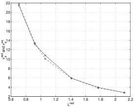
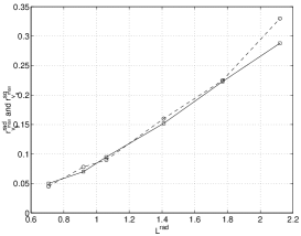
Figure 1: Comparison between results on square (squares and continuous line) and radial (circles and dashed line) integrations for: (a) $v_{\theta}^{\max}$ and (b) $r_{v_{\theta}^{\max}}$

A massive series of (automatic) radial integrations has been performed, since they are faster than GIANT. Both solutions and quasi-solutions are obtained and it is confirmed that the very precise results of the square integrations (GIANT) are points on a line of minimum error (12). They will be reported elsewhere.

4 Results

4.1 Summary of the numerical results

The strong nonlinear character of Eq.(1) combined with the internal procedures of GIANT (with no physical significance) imprints a particular structure to a space of functions that is explored for exact solutions. The space of functions representing initial conditions are divided into disjoint parts, such that from one subset one cannot access the final configuration of another subset. This means that in order to obtain a particular type of stationary (asymptotic) solution one has to initialize in a particular subset, homotopically connected to the final state. Most of the initial conditions does not lead to convergence and possibly they correspond to turbulent physical states. Exact solutions are obtained in the form of trivial ($\psi\equiv 0$) state and monopolar or multipolar vortices.

Besides exact solutions there are sets of functions that are almost solutions, i.e. velocity field configurations that verify the equation with only low accuracy and are normally rejected by the integration procedure at smaller tolerance. They are interesting because they appear systematically and approximately exhibit the same characteristics for a fixed $L$. The iteration of GIANT gets almost stuck around such a solution, which may suggest that they are metastable states of the physical fluid and eventually evolve slowly toward an exact solution, a smooth vortex. We call them quasi-solutions and we find useful to include them in our discussion. The main reason for accepting them as interesting and possibly physically relevant structures resides in the particularity of our approach: the fundamental object is the action functional and the configurations described by Eq.(1) extremize this action. If, by indifferently what method (here numerical), it has been possible to identify a configuration that seems to be very close to the extremum of the action (possibly a local minimum in the function space) then this configuration may play a role in the system’s evolution. Although a more detailed description of the structure of the function space around the extrema of the action is still required, the highly concentrated vortices identified numerically seem to be close of extremizing the action functional.

Restricting to the case of monopolar vortices we summarize the results by saying that for every $L$ we obtain two types of final vortices:

1. smooth, finite amplitude, vortices verifying the equation for any change in the accuracy of the integration procedure. There is a unique smooth vortex configuration for each $L$.

2. quasi-solutions, consisting of strongly localised vortices, with profiles for velocity and vorticity that are much narrower compared with the smooth vortices. These quasi-solutions are persistently obtained and they exhibit a clusterization around a typical shape for a particular $L$.

4.2 Solutions with the morphology of tropical cyclones

We are focusing here on the type of solutions that exhibit strong similarities with the morphology of a horizontal cross section of a tropical cyclone. These are circularly symmetric solutions with a strong maximum of the tangential velocity, strong concentration of vorticity.

We consider for ilustration the smooth, circularly symmetric vortex obtained for $L=1.25$. Fig.2 presents a section of the streamfunction $\psi\left(x,y\right)$ along the diagonal of the domain $\left(x,y\right)$. A section of the vorticity $\omega\left(x,y\right)$ is presented in Fig.3.

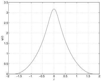
Figure 2: Solution $\psi(x,y)$ along the diagonal of the square, for the smooth vortex at $L=1.25$.

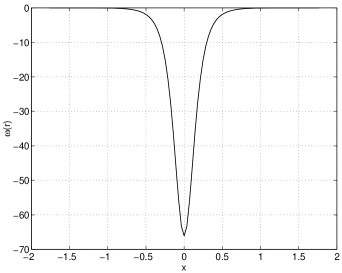
Figure 3: Vorticity calculated from $\psi(x,y)$ obtained by integration.

In order to quantify the accuracy of integration we collect in all the domain $\left(x,y\right)$ the pairs $\left(\psi,\omega\right)$ and plot them together with the line representing the nonlinear term in Eq.(1), Fig.4. The scatterplot of $\left(\psi,\omega\right)$ is almost superposed on this line. The scatterplot of the pairs [$\omega$, $-\frac{1}{2}\sinh\psi\left(\cosh\psi-1\right)$] (not shown) indicates a close clustering around the diagonal. Other tests are possible and they show that the integration is very good on most of the region and good within the imposed accuracy in the regions where the second derivative is very high.

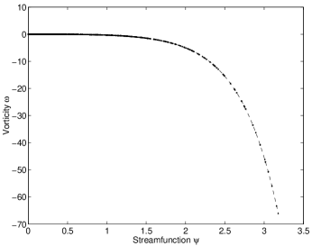
Figure 4: Scatterplot $(\psi,\omega)$, for the smooth vortex at $L=1.25$.

The tangential component of the velocity is shown in Fig.5. The steep descent to the center is clearly visible and its radial extension can be compared with the extension of the whole domain.

We have ploted in Fig.6 the section along the diagonal of the amplitude of the azimuthal component of the velocity.

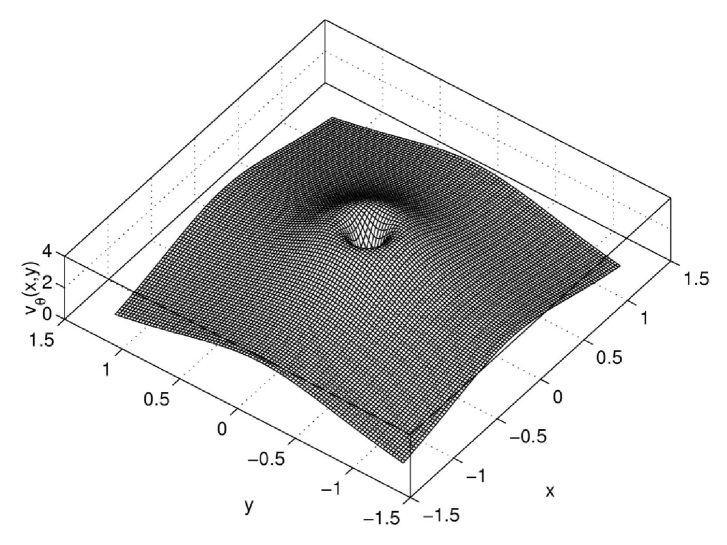
Figure 5: Azimuthal velocity $v_{\theta}(x,y)$ for the smooth vortex at $L=1.25$.

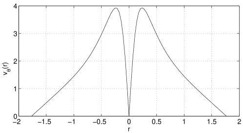
Figure 6: Azimuthal velocity $v_{\theta}(x,y)$ along the diagonal of the square of integration, for the smooth vortex at $L=1.25$.

Figure 7: Streamfunction $\psi(x,y)$ along the diagonal of the square of integration, for the quasi-solution at $L=1.25$.

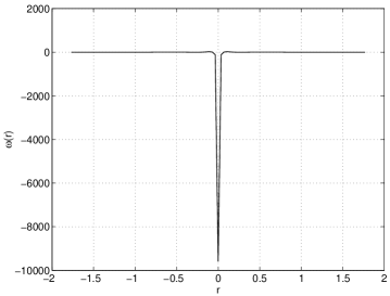
Figure 8: Vorticity $\omega(x,y)$ along the diagonal of the square of integration, for the quasi-solution at $L=1.25$.

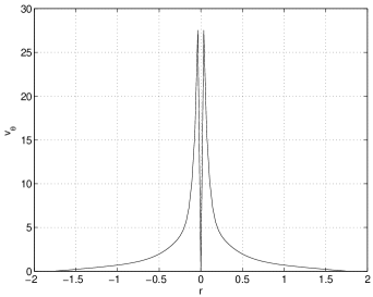
Figure 9: Azimuthal velocity $v_{\theta}(x,y)$ along the diagonal of the square of integration, for the quasi-solution at $L=1.25$.

In general the radial component of the velocity is much smaller than the azimuthal component. For this example ($L=1.25$) is in a ratio $\left|v_{r}\right|/\left|v_{\theta}\right|\sim 0.4/4=1/10$ and integrated over a circle shows no net inflow to the axis.

The large amount of results for the range of $L$ : $0<L\leq 10$, allows to formulate two remarks. First we note that for larger $L$ the profile of the azimuthal velocity shows smaller amplitude and larger radius of the circle of maximum velocity. Second, this variation with $L$ is much faster for low $L$ (less or comparable to $1$). The differences in the quantitative characteristics of the vortices for even small variation of $L$ in this range are substantial. Below we provide a scaling which shows exponential behavior, Eq.(13).

4.3 Quasi-solutions : strongly localised vortices

For comparison we present the profiles of the solution $\psi\left(x,y\right)$ Fig.7, vorticity $\omega\left(x,y\right)$ Fig.8 and azimuthal velocity $v_{\theta}\left(x,y\right)$ Fig.9 for the quasi-solution that correspnds to the same $L=1.25$. The sections are along the diagonal, denoted $r$. The results for every $L$’s seem to indicate a clusterization of the final total energy and final total vorticity. One should note that the total vorticity (obtained by integrating over the square) is however smaller than that for the corresponding smooth vortex shown in the preceding figures. The total energy $\frac{1}{2}\rho_{0}\int d^{2}r\left[\left(\mathbf{\nabla}\psi\right)^{2}+\frac{1}{\rho_{s}^{2}}\psi^{2}\right]$ for a fluid density $\rho_{0}$, is larger for the concentrated vortices compared to the smooth ones.

4.4 Quasi-solutions : multiple vortices

There are episodic structures of multiple vortices that are detected as solutions under a certain precision and which however evlove to symmetric monopolar vortex when the system is allowed to run further, under a higher precision.

It is worth to mention that in a numerical experiment we have identified a state where two vortices have been formed, placed in symmetrical positions along the diagonal of the square domain $L=0.5$. The initial function is trigonometric with periodicity $k=2$ with a coefficient $\psi_{0}=3.8$. Examining this structure with higher precision, after a longer iteration sequence the final solution was again the centered smooth vortex known for $L=0.5$. Therefore from the point of view of the numerical experience this state of two vortices is irrelevant. However, the persistence of this state inside the iterative search may indicate that it is close to a solution, possible less structurally stable.

Four vortices have been obtained in a run starting from trigonometric initial function. The initial function is trigonometric with periodicity $k=3$. The results show the formation of four vortices, as shown by Fig.10. Each of them has a structure that is similar to the one presented in Fig.2. It is interesting to note that again the vorticity is almost zero everywhere on the domain, except the regions of the four vortices, where it reaches very high values. The local tangential velocity presents the same very fast decay to the center of the vortex and each vortex is similar in structure with a typical cyclone.

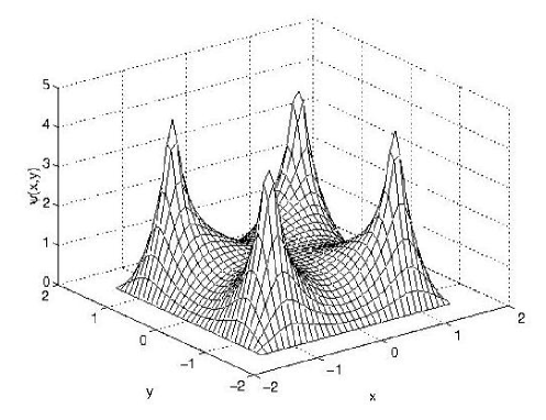
Figure 10: The scalar streamfunction $\psi(x,y)$ for a four-vortices solution.

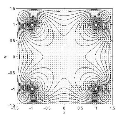
Figure 11: The contours of the scalar streamfunction $\psi(x,y)$ and the vector field $(v_{x}.v_{y})$ for a four-vortices solution.

5 Scaling laws inferred from numerical results

As mentioned before the nontrivial results of monopolar vortices are systematically of two types: a smooth vortex solution and a strongly localised quasi-solution. These are always the same for a fixed $L$. Their characteristics strongly depends on $L$, especially for the lower part of the range, where $L$ is few units or less.

Since the monopolar final states are independent of the initial conditions from which we start and of the particular numerical method of solution (GIANT) the relationships between the characteristics of the final vortices are objective and reflect properties of the equation itself. In addition the results (smooth vortex and narrow quasi-solution) are unique for a particular $L$, suggesting we can collect all numerical results in a form of nomograms or analytic (eventually spline functions) fit. However, we will look instead for analytic formulas which, even approximative, are simpler to use. We examine (a) the scaling of the maximum tangential velocity with the radius of the vortex, $R_{max}$; (b) the scaling of the radius of the eye-wall of the atmospheric vortex with the length $L$. Finally we will examine the existence of a linear relation between the energy and the vortictyin the final states.

5.1 The relationship between the maximal tangential velocity and the extension of the atmospheric vortex

We have inferred from numerical data an expression showing variation of $v_{\theta}^{\max}$ with the radial extension of the vortex $R_{\max}$

$$v_{\theta}^{\max}\left(L\right)\simeq\frac{e^{2}}{2}\left[\alpha\exp\left(\frac{\sqrt{2}}{R_{\max}}\right)-1\right]$$ (13)

for the interval $0<L=R_{\max}/\sqrt{2}<6$. This is shown in Fig.12.

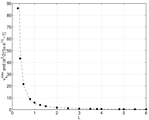
Figure 12: The maximum tangential velocity $v_{\theta}^{max}$ as function of $L=R_{\max}/\sqrt{2}$. The dashed line represents the fit according to Eq.(13)

For $\alpha=0.97$ this scaling works better for $L$ around $1$, and is a poor approximation over the range less than $0.4$. At $L\gtrsim 1.5$ this formula overestimates the maximum velocity and will not be used when we dispose, for the particular $L$, of the full numerical set as obtained by GIANT. However many observational data fall in the range $L\sim 1$ where Eq.(13) is a good fit and there it may be useful for a rapid estimation.

5.2 The relationship between the radius of the eye-wall and the extension of the atmospheric vortex

On the basis of many runs we have tried to infer a possible relationship between the radius of the eyewall, (the radius of the circle where the tangential velocity is maximum) and the parameter $L$.

When the data collected for a larger range of $L$, $0<L\leq 6$, is taken into account, it appears that there is an approximative linear dependence of $r_{v_{\theta}^{max}}\left(L\right)$ on $L=R_{\max}/\sqrt{2}$.

$$r_{v_{\theta}^{max}}\left(L\right)=0.11\left(-\frac{1}{2}+L\right)$$ (14)

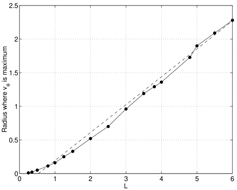
Figure 13: The radial position $r_{v_{\theta}^{\max}}$ where the tangential velocity $v_{\theta}^{max}$ attains its maximum, as function of $L$. The dashed line represents the linear fit according to Eq.(14)

As can be seen from Fig.13 this linear fit may present interest for a very wide range of $L$’s but it does not work well for low $L$, $0<L\lesssim 2.5$. Or this is the range that is relevant for the atmospheric vortex. It is necessary to look for a different fit for that range.

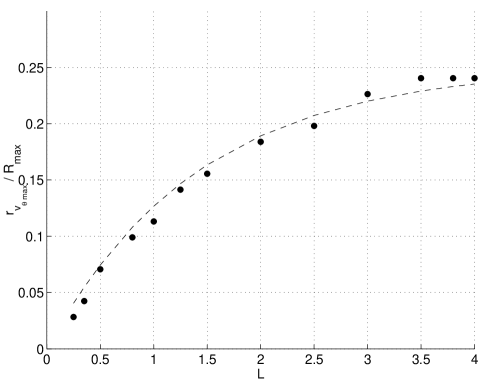
Figure 14: Ratio of the radius $r_{v_{\theta}^{\max}}$ where maximum of $v_{\theta}$ is attained to the radius of the maximum extension of the vortex, $R_{max}$ represented as function of the length $L=R_{\max}/\sqrt{2}$. The dashed line is the fit according to Eq.(15).

First we normalize the eye-wall radius to the radial extension of the vortex, $R_{max}\sim\sqrt{2}L$. Then the same numerical information can be organized to show the dependence of $r_{v_{\theta}^{max}}/R_{max}$ on the length $R_{\max}$. The following simple function offers a satisfactory fit for the low $L$ range

$$\frac{r_{v_{\theta}^{max}}}{R_{max}}=\frac{1}{4}\left[1-\exp\left(-\frac{R_{max}}{2}\right)\right]$$ (15)

Although it slightly overestimates the ratio (see Fig.14), this formula is practical by its simplicity and may be used for estimations based on observational data, as will be described later.

5.3 Energy and vorticity in the final states

The smooth and respectively the strongly concentrated vortices are persistently obtained, from a wide variety of initial conditions. This suggests that, apart variations due to the accuracy of the iteration process, these states really represent a stationary state and respectively a quasi-stationary state of the fluid. Their characteristics are completely determined once we have fixed the radial extension of the domain $R_{\max}$ or, for square integration, the length $L$, which is half the side of the square on which the integration is performed, with $\psi=0$ on its boundaries.

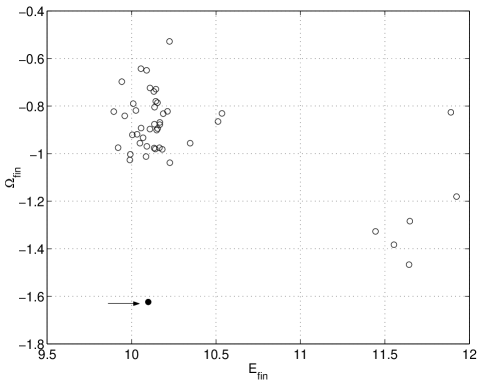
Figure 15: Energy and vorticity in the final states obtained at $L=1.25$. The dot indicated by the arrow consists of $84$ smooth vortices, while the $46$ narrow vortices (open circles) show a dispersion in energy and vorticity.

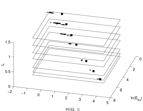
Figure 16: Energy and vorticity in the final states for several low $L$ values. The smooth (black squares) and concentrated vortices (small circles) are plotted in logarithmic scale. Every plane corresponds to a particluar $L$ value: $0.25$, $0.35$, $0.5$, $0.8$, $1.0$, $1.25$ and $1.5$.

In particular the final states for a fixed $L$ are characterised by two quantities, the total final energy and the total final vorticity and there are two pairs $\left(E_{fin},\Omega_{fin}\right)$: one for the smooth vortex and one for the narrow vortex. They are calculated with

$$E^{phys} = \rho_{0}^{phys}c_{s}^{2}\left(R_{\max}^{phys}/\sqrt{2}\right)^{2}$$

$$\times\frac{4}{n_{x}n_{y}}\frac{1}{2}\sum_{i=1}^{n_{x}}\sum_{j=1}^{n_{y}}\left[\left|v\left(i,j\right)\right|^{2}+\psi\left(i,j\right)^{2}\right]$$

where $\rho_{0}^{phys}$ is the density. We denote $E$ the energy $E^{phys}$ normalized to the physical coefficient in the first line above. The vorticity is

$$\Omega^{phys} = f_{0}$$

$$\times\frac{1}{n_{x}}\frac{1}{n_{y}}\sum_{i=1}^{n_{x}}\sum_{j=1}^{n_{y}}\omega\left(i,j\right)$$

When pairs $\left(E,\Omega\right)$are collected from all numerical experiences for a particular $L$, the precision of numerical determination of the solution is reflected in the dispersion of the points around an average one which may be supposed to be the exact solution. For the smooth vortices the dispersion is insignifiant, confirming that the numerical identification of this solution is very good, for all initializations. For the strongly localized vortex the dispersion is apparent and is connected with the higher magnitude of the second derivative on a very small area. However the results are clearly clustered around an average value which one can use to study various scaling relationships. This difference is exemplified in Fig.15 showing $130$ results for $L=1.25$, both smooth and narrow vortices, obtained from widely different initial conditions. The black dot indicated by the arrow actually consists of $84$ distinct dots representing almost identical results for the smooth vortex at $L=1.25$. The open circles are $46$ quasi-solutions narrow vortices, which have very close characteristics ($v_{\theta}\left(x,y\right)$, $r_{v_{\theta}^{\max}}$,etc.). They seem to represent approximations of a unique quasi-solution. The dispersion in the final energy and vorticity are a consequence of differences in the calculated second derivative of $\psi$ on a very small area, the reason for which they are actually rejected by GIANT. In Fig.16 data are plotted for several values of $L$.

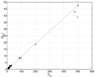
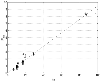
Figure 17: (a) Energy and vorticity in the final states corresponding to strongly localized vortices. The dashed line shows that there is a linear relationship between $E_{fin}$ and $\Omega_{fin}$. The figure (b) expands the region close to the origin.

The first important relation is between the energy $E_{fin}$ and the vorticity $\Omega_{fin}$ in the final states. The field theoretical model from which the equation is derived points out the existence of a lower bound for the energy functional for the point-like vortices: the energy is expressed as a sum of squared terms plus a supplementary term that has a topological content. The minimum of the energy is obtained by taking the squared terms to zero (and this leads to the self-dual equations and further to Eq.(1)) and this makes the energy equal to the topological term. Integrating over all plane this equality takes the form of a proportionality of the total energy and the total vorticity in the fluid motion. Therefore the numerical results collected for all $L$ should exhibit a linear relationship between $E_{fin}$ and $\Omega_{fin}$. Now we have for each $L$ two pairs $\left(E_{fin},\Omega_{fin}\right)$ and we can try to verify this linear relations for both. The total vorticity can be calculated easily in both cases, since the vorticity has a very good spatial limitation around the eye and decays rapidly to zero. The total energy Eq.(5.3) includes the integration of the squared velocity but the square domain of integration actually does not have everywhere zero velocity at the boundary, especially for higher $L$. Then a certain amount of energy cannot be included and $E_{fin}$ is not reliable. This is the case with almost all smooth vortices (except possibly the very small $L\sim 0.25...0.5$, where the localization of the smooth vortex is more pronounced). However, for the strongly localized vortices this problem does not arise, for any $L$. Fig.17 shows that there is indeed a linear relation between the energy and the vorticity. With lower accuracy (which we have mentioned before) the radial integrations confirm the proportionality of $E_{fin}$ and $\Omega_{fin}$.

5.4 The existence of a threshold in the initial energy and vorticity for obtaining a solution

Numerical simulations of basic fluid equations have shown that there is a boundary in the space of the initial configurations which separates two kinds of behaviors: on one side there are states from which the fluid evolves to random, turbulent states and on the other side there are initial configurations giving in long run organised, highly ordered flow with a vortical pattern. In the case of the Navier-Stokes equation this limit has been called the ergodic boundary by Deem and Zabusky (1971). In our case there is no time evolution and the iterations of GIANT have no particular physical meaning. We simply note however that a similar separation occurs in the present case. For any fixed $L$ the iteration of GIANT converges to a smooth vortex only if the amplitude of the initial function $\psi_{0}$ is higher than a particular value, depending on the peaking parameter $\delta$. This can be translated into a condition for the initial energy and vorticity. Choosing $L=1.25$ we have represented in Fig.18 the points $\left(E_{ini},\Omega_{ini}\right)$ corresponding to all types of final results: zero (asterisk), smooth vortex (open circles), narrow quasi-solution (black dots).

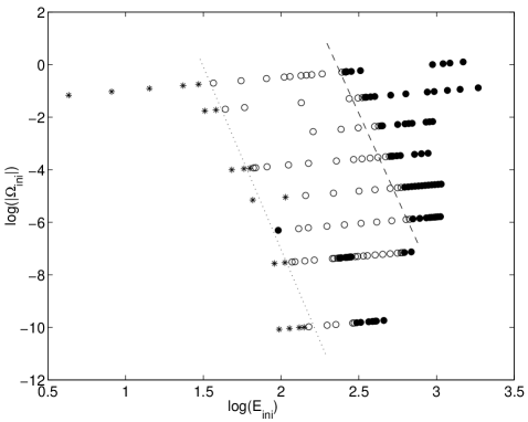
Figure 18: Set of points in the plane ($E_{ini},\Omega_{ini}$) from which the integrations for $L=1.25$ have been started, with the initial form Eq.(8). The points are distinguished according to the final states: (1) asterisks are initializations leading to trivial, zero, final state; (2) open circles are initializations leading to smooth vortex solutions; (3) black circles are initializations leading to quasi-solutions with strongly localised vorticity. The dotted line is a tentative separation of the trivial solutions (at left) from the smooth vortices (at right). The dashed line is an orientative separation of smooth from the strongly localised vortices. To the right of the righmost black circles there is no solution.

For purely orientative purpose a line is drawn, which approximately separates initial states leading to trivial solution $\psi\equiv 0$ (at left) from the initial states leading to smooth vortices (at right). This is very steep, $\Omega_{ini}-\Omega_{ini}^{0}\sim\left(E_{ini}-E_{ini}^{0}\right)^{-13.3}$ with $\left(E_{ini}^{0},\Omega_{ini}^{0}\right)$ one of the points on the limit. The other line is also orientative, separating the initial conditions leading to smooth (at left) and respectively strongly localised (at right) vortices.

5.5 Radial profile of the azimuthal velocity: comparison with Holland’s model

In an integration over square domain we obtain $\left(v_{x},v_{y}\right)$ with very good accuracy but the outer part of the field may be affected by the square geometry. For monopolar vortices we repeat the integration in radial geometry, which is extended over the length of the diagonal of the square, as explained. This profile can be compared with semi-empiric formulas like Holland’s or DiMaria. For the Holland’s model we use the formula

$$v_{\theta}^{H}\left(r\right)=\left\{\frac{b}{\rho_{0}}\left(\frac{r_{v_{\theta}^{\max}}}{r}\right)^{b}\left(P_{e}-P_{c}\right)\exp\left[-\left(\frac{r_{v_{\theta}^{\max}}}{r}\right)^{b}\right]+\frac{r^{2}f^{2}}{4}\right\}^{1/2}-\frac{rf}{2}$$

The parameters are: $b=2$ (the shape parameter), $P_{c}=990\,\left(hPa\right)$ (the pressure in the center of the vortex), $P_{e}=1015\,\left(hPa\right)$ (the environmental pressure), $\rho_{0}=1.15\,\left(kg/m^{3}\right)$, $f=5\times 10^{-5}\,\left(s^{-1}\right)$. The parameters used in this example correspond to

$$\left(r_{v_{\theta}^{\max}}\right)^{phys}\simeq 10\,\left(km\right)\;,\;R_{\max}^{phys}=95\,\left(km\right)$$

and this can be taken as starting point of our calculations based on Eq.(1) and the scaling laws derived from it. We calculate the ratio of the two distances $r_{v_{\theta}^{\max}}^{phys}/R_{\max}^{phys}=10/95=0.1053$. We insert this value in the scaling described by Eq.(15) and determine the maximum radial extension of the vortex (normalised), $R_{\max}$

$$\frac{1}{4}\left[1-\exp\left(-\frac{R_{\max}}{2}\right)\right]=\frac{r_{v_{\theta}^{\max}}}{R_{\max}}=\frac{r_{v_{\theta}^{\max}}^{phys}}{R_{\max}^{phys}}=0.1053$$

From here we obtain

$$R_{\max}=1.0931$$ (18)

or, equivalently $L^{sq}=R_{\max}/\sqrt{2}=0.7729$. The Rossby radius, is

$$\rho_{g}=\frac{R_{\max}^{phys}}{R_{\max}}=\frac{95\;\left(km\right)}{1.0931}=86.9\;\left(km\right)$$

This is the first physical unit that we need in order to translate our numerical results (normalised quantities) into physical quantities. The unit of vorticity is $f_{0}=5\times 10^{-5}\;\left(s^{-1}\right)$ and the unit of velocity

$$\overline{v}=\rho_{g}f_{0}=86.9\times 10^{3}\times 5\times 10^{-5}\simeq 4.34\;\left(m/s\right)$$

The numerical solution of Eq.(1), obtained with the code BVPLSQ in circular symmetry for $L^{rad}\equiv R_{\max}=1.0931$ , gives

$$v_{\theta}^{\max}\simeq 9$$

This result is confirmed by the integration on the square domain $L^{sq}=R_{\max}/\sqrt{2}=0.7729$, with GIANT, where we obtain $v_{\theta}^{\max}\simeq 9.5$. As explained before, the integration over the square domain is more precise compared with the radial one (GIANT versus BVPLSQ). However to compare with the profile of Holland’s model, we take the result of the radial integration. We can now calculate this velocity in physical units

$$\left(v_{\theta}^{\max}\right)^{phys}=4.34\,\left(m/s\right)\times 9\simeq 39.11\;\left(m/s\right)$$

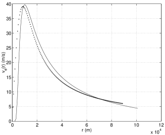
Figure 19: Azimuthal velocity from the Holland model (continuous line) and from Eq.(1) (circles).

The Holland’s model gives approximately $39.73\;\left(m/s\right)$. In addition we plot in Fig.19 the radial profiles of the azimuthal velocity from the Holland’s model (continuous line) and from our Eq.(1) (dotted line), in physical units. The similarity of profiles is apparent. We note however that these profiles are senzitive to choices that are difficult to measure in observation: for the Holland’s model the parameters, in particular $b$, are affected by imprecisions. For our model, the main physical input is the radius of the eye wall and the maximum extension of the cyclone and these are equally affected by imprecisions.

6 Practical application of the scaling laws

In this section we discuss how to use the scaling relations we have derived when we want to compare with a real observational data of a tropical cyclone. Since for a fixed $L$ the integration provides a unique smooth vortex, all data regarding this vortex are available in the form of functions : $\psi\left(x,y\right)$, $\omega\left(x,y\right)$, $v_{\theta}\left(x,y\right)$, and derived quantities : $r_{v_{\theta}^{\max}}$, $v_{\theta}^{\max}$, $E_{fin}$, $\Omega_{fin}$. All are normalized and the first task is to identify the physical units that will relate these quantities to the physical data. Basically there are two units: $\rho_{g}$ and $f_{0}$ and the latter is assumed known.

A possible starting point is to estimate (from observations) the ratio between the radius of the circle of maximum azimuthal velocity $r_{v_{\theta}^{\max}}^{phys}$ and the radius of the minimum disc containing the cyclone, $R_{\max}^{phys}$ (here as usual the upperscript phys means that the quantities are dimensional). Suppose this ratio can be estimated on the basis of a satelite picture. Then we can use Eq.(15) or Fig.13 to identify the parameter $L$. Since a real-life observation provides also the physical radius of the cyclone, $R_{\max}^{phys}$ we can determine the Rossby radius from: $R_{\max}^{phys}=\sqrt{2}L^{phys}=\sqrt{2}\rho_{g}L$ where we use $L$ as determined. Then the unit of the physical quantities are calculated : $\rho_{g}f_{0}$ for velocity and $\rho_{g}^{2}f_{0}$ for the streamfunction. From the runs of the code for $L$ we dispose of profiles for all (normalized) variables. Using the units we can calculate some characteristics that can be further compared with the observations: the maximum azimuthal velocity $v_{\max}^{phys}$, the profile of the velocity, the vorticity, etc.

6.1 Example 1

We use pictures of the profile of the mean tangential wind for the hurricane Andrew, according to Willoughby and Black (1996). In Fig.3b of this reference it is represented the west to east wind profile before the eyewall replacement (23 August 1665 UTC). We retrieve the approximate values: $v_{\theta\max}^{phys}\simeq 68\,\left(m/s\right)$, $r_{v_{\theta}^{\max}}^{phys}\simeq 12\,\left(km\right)$ and we assume (with a certain extension beyond the limits presented in the figure) $R_{\max}^{phys}\simeq 120\,\left(km\right)$. From this we calculate

$$\frac{r_{v_{\theta}^{\max}}^{phys}}{R_{\max}^{phys}}\simeq\frac{12}{120}=0.1$$ (19)

With this value we turn to Eq.(15) to calculate $R_{\max}$ and then $L$.

$$\frac{1}{4}\left[1-\exp\left(-\frac{R_{\max}}{2}\right)\right]=\frac{r_{v_{\theta}^{\max}}}{R_{\max}}=\frac{r_{v_{\theta}^{\max}}^{phys}}{R_{\max}^{phys}}=0.1$$ (20)

with the result

$$R_{\max}\simeq 1.0217\;,\;L\simeq 0.72$$ (21)

Taking $L=0.72$, we have at this moment at our disposal all the set of results that are obtained numerically for the smooth vortex at this $L$. Coming back to the physical data we now use the spatial extension of the vortex, $R_{\max}^{phys}\simeq 120\,\left(km\right)$ to calculate the Rossby radius $\rho_{g}$, i.e. the space normalization

$$\rho_{g}=\frac{R_{\max}^{phys}}{\sqrt{2}L}=\frac{120}{\sqrt{2}\times 0.72}\simeq 117.85\,\left(km\right)$$

Now we can calculate the other physical units: $\overline{\omega}=f_{0}=5\times 10^{-5}\;\left(s^{-1}\right)$ (from Emanuel 1989, Table 1), for velocity $\rho_{g}f_{0}=5.9\,\left(m/s\right)$, for streamfunction $\rho_{g}^{2}f_{0}=0.694\times 10^{6}\,\left(m^{2}/s\right)$. By numerically solving Eq.(1) for $L=0.72$ we find $v_{\theta}^{\max}=10.9$. Note that the Eq.(13) gives a close value: $10.67$. The physical value results $v_{\theta}^{\max}=64.31\,\left(m/s\right)$. This is comparable to $68\,\left(m/s\right)$ the value shown by Willoughby and Black. The maximum vorticity is $\left|\omega_{\max}\right|=491.2\times f_{0}=0.0246\,\left(s^{-1}\right)$.

6.2 Example 2

For this example we adopt the following input data: the ratio of the full spatial extension of the hurricane to the radius of maximum tangential wind is $R_{\max}^{phys}/r_{v_{\theta}^{\max}}^{phys}\sim 9$; and the physical extension of the hurricane is $R_{\max}^{phys}\sim 300\,\left(km\right)$. The data can be compared with the picture taken by NASA at 28 August 2005, when the hurricane Katrina was above the Mexic gulf, but the identification of physical data is certainly approximative. Eq.(15) is used to find

$$L\sim\frac{1}{\sqrt{2}}\left(-2\right)\ln\left(1-4\frac{r_{v_{\theta}^{\max}}^{phys}}{R_{\max}^{phys}}\right)=0.8313$$

It results the Rossby radius $\rho_{g}=R_{\max}^{phys}/\left(\sqrt{2}L\right)\sim 212\,\left(km\right)$. The unit of vorticity is the Coriolis parameter $\overline{\omega}=f_{0}=5\times 10^{-5}\;\left(s^{-1}\right)$ and we have the unit of velocity $\overline{v}=\rho_{g}\overline{\omega}=10.6\;\left(m/s\right)$ . Looking again to the results from the numerical integration for $L=0.83$ we find the magnitude of the normalized tangential velocity $v_{\theta}^{\max}=8.37$ (note that Eq.(13) gives a similar value, $8.26$), which means that in physical units we have

$$v_{\theta\max}^{phys}\sim 88.6\;\left(m/s\right)$$

This gives a very high value for the maximum tangential wind, but the range is still realistic. The maximum vorticity is $\left|\omega_{\max}\right|=290.38\times f_{0}=0.0145\,\left(s^{-1}\right)$.

6.3 Example 3

We take for the third example the approximative value $R_{\max}^{phys}/r_{v_{\theta}^{\max}}^{phys}\sim 8$ and a radius of maximum extension of the hurricane of $R_{\max}^{phys}\sim 350\;\left(km\right)$. (This is inspired by the picture taken by NASA on the hurricane Rita, September 21, 2005). From this data it is obtained

$$L\sim\frac{1}{\sqrt{2}}\left(-2\right)\ln\left(1-4\frac{r_{v_{\theta}^{\max}}^{phys}}{R_{\max}^{phys}}\right)=0.9803$$

Then we can calculate the Rossby radius $\rho_{g}=R_{\max}^{phys}/\left(\sqrt{2}L\right)=252.47\;\left(km\right)$. Taking the Coriolis parameter $f_{0}=5\times 10^{-5}\;\left(s^{-1}\right)$ we have the physical unit of velocity $\overline{v}=\rho_{g}\overline{\omega}=12.6\;\left(m/s\right)$ . The maximum tangential velocity for $L=0.98$ can be calculated using the scaling formula Eq.(13), with the result $v_{\theta}^{\max}=6.24$. We will use however the exact result, provided by numerical integration with GIANT of Eq.(1), $v_{\theta}^{\max}=6.15$ and this leads to the physical velocity

$$v_{\theta\max}^{phys}=77.5\;\left(m/s\right)$$

The maximum vorticity is $\left|\omega_{\max}\right|=158.34\times f_{0}=0.0079\,\left(s^{-1}\right)$.

These examples confirm the possibility of using the scaling relationships Eq.(13) and Eq.(15) to estimate the physical charactersistics of the tropical cyclone. We note that the results of the estimations can be significantly affected by the approximations on the observational data, especially that of the ratio $r_{v_{\theta}^{\max}}/R_{\max}$. This is because the magnitude of $L$ which is obtained from Eq.(15) using a reasonable input value for this ratio belongs to a range where the variations with $L$ of all the characteristics of the solution ($\psi$, $\omega$, $v_{\theta}$, $r_{v_{\theta}^{\max}}$) are substantial. It is sufficient to look at the dependence of $v_{\theta}^{\max}$ on $L$, Fig.11.

7 Discussion

At the origin of our approach it is the Charney-Hasegawa-Mima model, a two-dimensional, nondissipative and purely fluid-dynamical (no thermal process) model. Although is a simplified model it exhibits (via the field-theoretical formulation) a compact analytic and algebraic structure, self-duality, leading to Eq.(1). We have several arguments in favor of the conclusion that Eq.(1) may represent the fluid nonlinear-dynamic part of the atmospheric vortex. First, the profiles obtained by solving Eq.(1) are similar to results already known (from observations or numerical simulation) for the same quantities.

1. The profile of the the tangential velocity, our Fig.5, is similar to typical tropical cyclone velocity profiles, as represented in Fig.2 of Wang and Wu 2004. This is also confirmed by close similarity with the Fig.1a from Reasor and Montgomery 2001 and with the profile given by the Holland model or with the experimental observation (for Andrew hurricane, Willoughby and Black 1996).

2. The fast decay to zero of the vorticity $\omega$ shown in our Fig.2 is similar to what is shown in Fig.1a of Kossin and Schubert 2001; ideally (without dissipation and friction) for mature hurricanes the maximum of $\omega$ is on the center.

3. We note that in  a series of reported numerical simulations, the tendency of the fields is to evolve toward profiles that are very close to those shown in our figures 2 and 5. For example, the Fig.7a and 7b of Kossin and Schubert 2001 show the evolution of the vorticity and mean of the tangential velocity from initial profiles which correspond to a narrow ring of vorticity to profiles that show clear ressemblance with our figures 2 and 5. The same striking evolution to profiles similar to ours appears in Figs.7 a and b of the same Reference. We have investigated whether a radially annular profile of vorticity can be a solution of our equation (1). The result is negative, which may explain why such an initial profile evolves to either a set of vortices (vortex-crystal) or to a centrally peaked structure as in Fig.2.

Second, we obtain a good consistency between our quantitative results for an atmospheric vortex (using approximative input information) and the values measured or obtained in numerical simulations.

Finally, the quasi-solutions which appear to be an interesting feature of this equation, are compatible with a series of previously known results: the four vortices represented in our figure 10 are similar to the Figure 4a from the work of Kossin and Schubert 2001. And the evolution to a monopolar structure we obtain is similar to the same process reported in this reference.

The numerical results have made possible to formulate several scaling relationships connecting parameters of the atmospheric vortex. These are simple formulas, intended for practical use, inevitably approximative. This is because our purpose was to infer an analytical expression for a curve which is determined numerically (or: is known in the form of a simple table of values). Other expressions are possible and are worth to look for. A true scaling law will become possible only as a result of an analytical  investigation of the properties of the equation. On the other hand, this equation does not have a Backlund transform and is probable not integrable by the Inverse Scattering Transform.

An important field of future investigation (analytical and numerical) is represented by the quasi-solutions, elements of a space of functions that are very close of verifying the equation. Are they close to the extremum of the action functional of the full field-theoretical model, for example, are they metastable states? From the physical point of view it may result that these states can be rendered more stable by processes that are connected with what is missing from the Charney-Hasegawa-Mima model: third dimension, viscosity, thermal processes. It is worth to examine the role of the strongly localized quasi-solutions in models of tornadoes.

An interesting suggestion results from the massive series of radial integrations: it appears that in the space of functions there are strings of vortical quasi-solutions emanating from the exact solution and showing increasing degree of departure from exactness (increase of the $error$ functional). If some physical factor will provide stability to these quasi-solutions, then the system may slide along this string, with the consequence that there is no pure stationarity but a continuous evolution to stronger and stronger localisation of the vortex. This requires further study.

Developing from the present one, a future self-consistent model will have to include variation of the Rossby radius with the dynamical properties of the vortex. Since this implies to consider that the coefficient of the Chern-Simons part in the Lagrangian is a nonlinear function of the scalar field, it is difficult to say if the self-duality will be maintained.

The investigation of this equation, and, most important, of the field-theoretical model from which it is derived, are worth to be continued.

Acknowledgments. This work has been partly supported by the Romanian Ministry of Education and Research and by the Japan Society for the Promotion of Science. The hospitality of Professor S.-I. Itoh and of Professor M. Yagi at the Kyushu University is gratefully acknowledged.

References

- [Charney 1948] Charney, J. G., 1948. Geophys. Public. Kosjones Nors. Videnshap. Akad. Oslo. 17:3.
- [Hasegawa and Mima 1978] Hasegawa, A. and Mima K., 1978. Pseudo-three-dimensional states in magnetized nonuniform plasmas. Phys. Fluids 21:87-92.
- [Horton and Hasegawa 1994] Horton, W. and Hasegawa A., 1994. Quasi-two-dimensional dynamics of plasmas and fluids. Chaos 4:227-251.
- [Matthaeus et al. 1991a] Matthaeus, W.H., Stribling W.T., Martinez D., Oughton S. and Montgomery D., 1991. Selective decay and coherent vortices in two-dimensional incompressible turbulence. Phys. Rev. Lett. 66:2731-2734.
- [Matthaeus et al. 1991b] Matthaeus, W.H., Stribling W.T., Martinez D., Oughton S. and Montgomery D., 1991. Decaying, two-dimensional, Navier-Stokes turbulence at very long times. Physica D51:531-538.
- [Kinney et al. 2005] Kinney, R., McWilliams J. C. and Tajima T., 1995. Coherent structures and turbulent cascades in two-dimensional incompressible magnetohydrodinamic turbulence. Phys. Plasmas 2:3623-3639.
- [Spineanu and Vlad 2005] Spineanu, F. and Vlad M., 2005. Stationary vortical flows in two-dimensional plasma and planetary atmospheres. Phys.Rev.Lett. 94:235003-1-4.
- [de Rooij et al. 1999] de Rooij, F., Linden P. F. and Dalziel S. B., 1999. Experimental investigations of quasi-two-dimensional vortices in a stratified fluid with source-sink forcing. J. Fluid Mech. 383:249-283.
- [Seyler 1996] Seyler, C.E., 1996. On the most probable states of two-dimensional plasma. J. Plasma Physics 56:553-567.
- [Emanuel 1986] Emanuel, K.A., 1986. An air-sea interaction theory for tropical cyclones. Part I. J. Atmos. Sci. 43:585-604.
- [Emanuel 1989] Emanuel, K.A., 1989. The finite-amplitude nature of tropical cyclogenesis. J. Atmos. Sci. 43:3431-3456.
- [Reasor and Montgomery 2001] Reasor, P.D. and Montgomery M. T., 2001. Three-dimensional alignement and corotation of weak, TC-like vortices via linear vortex Rossby waves. J. Atmos. Sci. 58:2306-2330.
- [Kossin and Schubert 2001] Kossin, J. P. and Schubert W. H., 2001. Mesovortices, polygonal flow patterns, and rapid pressure falls in hurricane-like vortices. J. Atmos. Sci. 58:2196-2209.
- [Yatsuyanagi 2005] Yatsuyanagi, Y., Kiwamoto, Ya., Tomita H., Sano, M.M., Yoshida, T., Ebisuzaki, T., 2005. Dynamics of two-sign point vortices in positive and negative temperature states. Phys. Rev. Lett. 94:054502-1-4.
- [Morikawa 1960] Morikawa, G. K., 1960. Journal of Meteorology. 17:148-158.
- [Stewart 1943] Stewart, H. J., 1943. Q. Appl. Math. 1:262-267.
- [Willoughby and Black 1996] Willoughby, H. E. and Black P.G., 1996. Hurricane Andrew in Florida: dynamics of a disaster, Bull. Amer. Meteor. Soc. 77:543-549.
- [Wang and Wu 2004] Wang, Y. and Wu C.-C., 2004. Current understanding of tropical cyclone structure and intensity changes - a review. Meteorol. Atmos. Phys. 87:257-278.
- [Fyfe 1976] Fyfe, D., Montgomery D. and Joyce G., 1976. J. Plasma Phys. 17:369-.
- [Kraichnan and Montgomery 1980] Kraichnan, R. H., and Montgomery D., 1980. Rep. Prog. Phys. 43:547-619.
- [Montgomey and Joyce 1974] Montgomery, D. and Joyce G., 1974. Phys. Fluids 17:1139-1145.
- [Joyce and Montgomery 1973] Joyce, G. and Montgomery D., 1973. J. Plasma Phys. 10:107-.
- [Montgomery et al. 1992] Montgomery, D., Matthaeus W.H., Stribling W.T., Martinez D. and Oughton S., 1992. Relaxation in two-dimensions and the “sinh-Poisson” equation, Phys. Fluids A4:3-6.
- [Spineanu and Vlad 2003] Spineanu F. and Vlad M., 2003. Self-duality of the asymptotic relaxation states of fluids and plasmas. Phys. Rev. E67:046309, 1-4.
- [Spineanu et al. 2004] Spineanu, F., Vlad M., Itoh K., Sanuki H. and Itoh S.-I., 2004. Pole dynamics for the Flierl-Petviashvili equation and zonal flows. Phys. Rev. Lett. 93:025001-1-4.
- [Nowak and Weimann 1990] Nowak, U. and Weimann L., 1990. GIANT A software package for the numerical solution of very large systems of highly nonlinear equations, Konrad-Zuse-Zentrum fur Informationtechnik Berlin, Technical Report TR 90-11.
- [Deeam and Zabusky 1971] Deem, G. S. and Zabusky N. J., 1971. Ergodic boundary in the numerical simulation of two-dimensional turbulence. Phys. Rev. Lett. 27:396-399.